1. Introduction
Mesoscale eddies have gained considerable research attention, both from oceanographic and acoustic viewpoints. These eddies can be classified into two main types based on their vertical distribution of hydrographic signals: surface eddies and subsurface eddies. Surface eddies typically exhibit strong signals at the surface, making them easily detectable through satellite data. On the other hand, subsurface eddies are characterized as rotating and translating bodies of water found within the intermediate or deeper layers of the ocean. Subsurface eddies have been identified in various regions of the global ocean, using data from Argo floats and occasional in situ observations. Previous reports suggest that most subsurface eddies occur in geographically preferred regions, e.g., Meddies in the Mediterranean Sea [
1,
2,
3], Ruddies in the Indian Ocean [
4], Cuddies near the California Undercurrent [
5,
6,
7], and Puddies in the Southeast Pacific Ocean [
8,
9,
10,
11]. The significant influence of subsurface eddies on physical properties is that they can powerfully change the subsurface circulation, pathways of water masses, and redistribution of heat, salt, and momentum [
12]. There are usually differences in temperature and salinity between the subsurface eddies and background water. These discrepancies usually lead to alterations in the sound speed profile across the eddies. As a consequence, the acoustic propagation is subsequently disturbed.
Comprehending acoustic propagation through mesoscale eddies can enhance the accuracy of sonar and communication system predictions, facilitate strategic placement of acoustic equipment, and contribute as an input to navigational path-planning algorithms. Recognizing this importance, early studies, starting from the 1970s, have studied different aspects of acoustic propagation through mesoscale eddies. Gemmill and Khedouri [
13] demonstrated that cold eddies in the Sargasso Sea have a pronounced effect on sound propagation using a ray tracing model; Vastano and Owens [
14] studied the acoustic properties of a cyclonic Gulf Stream ring with field data and ray computation. Nysen et al. [
15] investigated sound transmission through an East Australian Current summer eddy and found that the eddy caused an elongation of the convergence zone range by 8 km. Baer [
16] studied propagation through a three-dimensional model of an eddy using a parabolic-equation numerical approach. They examined the impact of the eddy on Transmission Loss (TL) in both the vertical and horizontal planes. Results showed that refractive variations caused a 20 km difference in the range of a given acoustic feature. Henrick et al. [
17] examined the impact of sound speed and current fluctuations caused by a mesoscale cyclonic eddy on short-range propagation. They examined the influence of an eddy on travel time and sound rays. Lawrence [
18] studied the effect of warm eddies on acoustic propagation. The influence of the eddy border on convergence zone parameters was demonstrated to be substantial. Kevin and Richard [
19] discovered that the refraction caused by mesoscale oceanography, including fronts and mesoscale eddies, could substantially affect the localization of distant low-frequency sources, such as seismic or nuclear test events. Overall, previous research is mainly based on a singular profile or an idealized eddy model constructed using a collection of parameters. However, the description of these sound speed fields is not complete and adequate enough to include all the major determining features of acoustic transmission.
The sound speed distribution within subsurface eddies presents a unique set of challenges due to its distinctive lens-like shape, dynamic nature, and spatial distribution patterns. Recent statistical analyses and in situ data have provided compelling evidence for the prevalence of subsurface eddies across the northwestern Pacific Ocean [
20,
21]. These eddies are typically generated by the subduction of mode water or the instability of oceanic jets [
22,
23]. Despite the valuable insights gained from studying the impact of subsurface eddies on various physical oceanographic properties, limited research has been devoted to investigating the specific characteristics of acoustic fields influenced by these eddies. In contrast to previous studies that primarily focus on oceanographic features, this paper aims to explore the effects of acoustic propagation resulting from a large subsurface eddy situated southeast of Taiwan in the northwestern Pacific Ocean. To achieve this, a comprehensive simulation study was conducted employing a ray tracing model.
In this paper, the organization is as follows.
Section 2 provides a concise overview of the subsurface eddy, highlighting both its hydrological characteristics and sound speed structure.
Section 3 compares and contrasts the findings obtained under eddy conditions with those obtained in the absence of eddies. Lastly,
Section 4 presents a comprehensive summary of the key results.
3. Results and Discussion
Numerical simulation results are presented in this section, where the observed oceanographic eddy field is compared to the climatology field using a ray tracing model. The aim is to evaluate the influence of the subsurface eddy on acoustic propagation. Propagations both into and out of the eddy are considered. The effects of source depth variation on acoustic propagation are also examined.
3.1. Modeling Setting
A comprehensive numerical study of acoustic propagation in the previously discussed subsurface eddy was carried out by Bellhop. It is a beam-tracing model for predicting acoustic pressure fields in ocean environments. Bellhop can successfully handle variations in sound speed profiles with horizontal distance (range). Additionally, it permits the consideration of range dependence in the upper and lower bounds. Readers interested in the detailed information about the ray tracing model are referred to Porter et al. [
26,
27].
In the 23° N section, the average depth exceeds 5000 m, and the topography is relatively flat. This indicates that the eddy experiences minimal influence from the topography. Therefore, when considering environmental parameters for the sound propagation model, the topography was ignored. The sediment bottom in the model is assumed to be a half-space with specific properties. The sound speed, density, and bottom attenuation of the sediment are set at 1600 m/s, 1.8 g/cm3, and 0.4 dB/λ, respectively. These values represent the acoustic characteristics of the sediment layer in the modeling simulation. The acoustic frequency used in this investigation was 300 Hz.
It is important to note that the XCTDs provide temperature and salinity data up to a depth of 800 m. It is still far from the sea bottom. To obtain complete profiles to the bottom, which is essential to calculate the acoustic field, the sound speeds were extended from 800 m (the deepest XCTD data point) to the seafloor, using climatological data for the 23° N section from WOA13. Prior to combining the two data types, it was necessary to apply smoothing near the 800 m depth to ensure seamless integration.
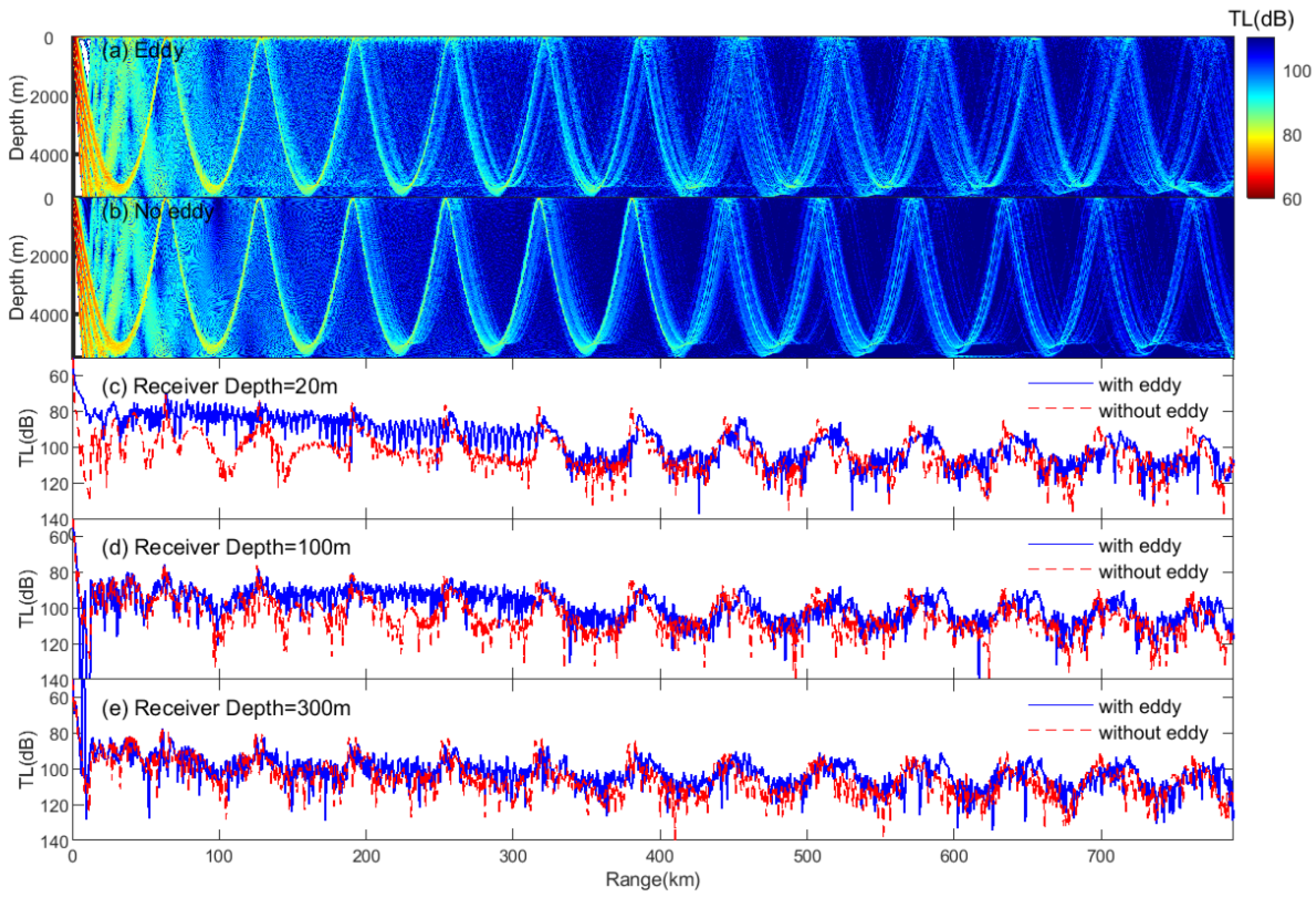
3.2. Propagation into the Eddy
In this section, the sound source at a frequency of 300 Hz was situated at zero range, about 180 km from the left edge of the vortex, propagating over a total horizontal range of 790 km. The distance between the eddy center (126° E, 23° N) and the sound source was approximately 410 km. The large distance between the source and the eddy was chosen to include the whole eddy boundary. It connects surrounding water to the subsurface eddy and is proven to have significant effects on convergence zone properties [
18]. We compared the TL from a source at 122° E, 23° N, passing through the subsurface eddy discussed earlier, with the TL from the same source passing through the same geographical region without the eddy. The sound speed without the eddy was calculated using the climatological temperature and salinity in the same section derived from WOA13.
3.2.1. TL Difference
Figure 4 illustrates the difference between the TL between the presence and absence of the eddy. Considering different source depths. Note that a negative TL is associated with an energy gain. The subsurface eddy extends from 180 to 640 km in the horizontal plane.
The deployment of the sound source at different depths allows for a comprehensive assessment of the impact of the subsurface eddy on acoustic propagation. The source is deployed at different depths, from the surface to deeper ocean layers. Source depths of 20 m, 100 m, 460 m, and 800 m are selected corresponding, respectively, to cases of the source being in the mixed layer, a source in the subsurface layer, a source at the depth where the sound speed varies the most, and a deeper source displayed for contrast.
There are several features of the TL difference that are of interest: (1) When the source is placed in 20 m, the eddy perturbation produces TL changes on the order of 10–20 dB in the mixed layer and within the range of 320 km; (2) When the source is around 100 m, there are 20–30 dB changes in the convergence zone paths primarily due to shifting of the TL patterns between the eddy and no-eddy cases; (3) When the sound source is below 150 m, the subsurface eddy has a negligible effect on acoustic propagation. The details that illustrate these points will be discussed further.
3.2.2. Source at 20 m
For the source within the mixed layer depth, detailed TL plots for the source depth of 20 m in the eddy and no eddy cases are displayed in
Figure 5. A characteristic pattern of deep-water convergence zone can be observed, where the sound energy carried by water fluctuates between the channel’s upper and lower sections.
Although
Figure 5a,b are superficially similar, there are significant quantitative and qualitative differences where the eddy exists. The most important distinction is that the presence of the eddy supports robust propagation in the surface duct, leading to a high sound level near the surface, while the absence of the eddy does not.
To provide a clearer picture of the distribution of the surface duct,
Figure 5c–e depict TL curves at different receiver depths (20 m, 100 m, and 300 m). The solid blue line indicates TL for the subsurface eddy, while the red dashed line indicates no eddy. The results demonstrate that the surface duct holds at least the range of approximately 320 km and vanishes at about 100 m depth when the subsurface eddy exists. In contrast, convergence zones are the only propagation mode in the absence of eddies.
The modification of the sonic layer depth due to the subsurface eddy explains its impact on sound transmission within the surface duct, where the acoustic energy could travel long distances. The sonic layer depth is an important factor in acoustic channels. It is computed by finding the subsurface maximum sound speed. Variability of the sonic layer depth is the essential factor affecting acoustic propagation in the upper layer [
28,
29].
Vertical gradients of sound speed in the upper layer with and without eddy across the 23° N section are shown in
Figure 6a and
Figure 6b, respectively. In the eddy plot, sound speed increases with depth in the upper 40 m layer and within 320 km. Vertical gradients of sound speed create a surface sound duct. Notably, the sonic layer depth varies at different distances: 38 m at 0 km, 51 m at 180 km, and 0 m at 400 km, indicating the complete disappearance of the sonic layer at the eddy center. Consequently, the subsurface eddy exerts a significant influence on the surface acoustic channel by altering the sonic layer depth. Conversely, in the absence of an eddy, a negative vertical gradient is observed within the upper layer up to a depth of 100 m. As the depth increases, the sound velocity generally decreases, resulting in the absence of a sonic layer.
3.2.3. Source at 100 m
We now consider a deeper source of 100 m in the same environment as the 20 m case. Several characteristics are illustrated by these plots of the TL (
Figure 7). First, with a source at this depth, propagation can be seen to still exhibit recurring convergence zones, but it does not support mixed layer propagation whether the eddy exists or not.
Second, a given convergence zone is deflected away from the sound source in the presence of the eddy. There are 12 convergence zones within 790 km in
Figure 7. In response to the immense sound speed gradient caused by the eddy, the sinusoidal region’s peaks and troughs become approximately 60° out of phase between the two plots in
Figure 7a,b at 700 km, with the eddy case lagging.
Finally, receiver depth selection is very important in surveillance. For the shallower receiver depth of 20 m, corresponding to
Figure 7c, the TL curves are quite similar. Thus, the eddy has little effect on propagation near the surface. When the receiver is deployed at the same depth as the source (
Figure 7d), TL changes caused by the subsurface eddy are up to 25 dB. As propagation waves enter the left side of the eddy, at approximately 200 km, convergence zones tend to change their ranges, and their territories no longer overlap from 480 km due to the acoustic properties of the subsurface eddy.
To assist in discussing these results,
Table 1 provides a range of convergence zone parameters extracted from
Figure 7d. However, for brevity, the table begins documenting these parameters from the fourth convergence zone onwards. It should be emphasized that the first three convergence zones in both water types exhibit remarkably similar characteristics, appearing at approximately 60, 121, and 183 km, respectively, with comparable energy levels. It is worth noting that as the distance increases, the separation between corresponding convergence zones also widens. The difference in position of convergence zones reaches 14 km for the tenth convergence zone. These results can be of great importance for underwater surveillance.
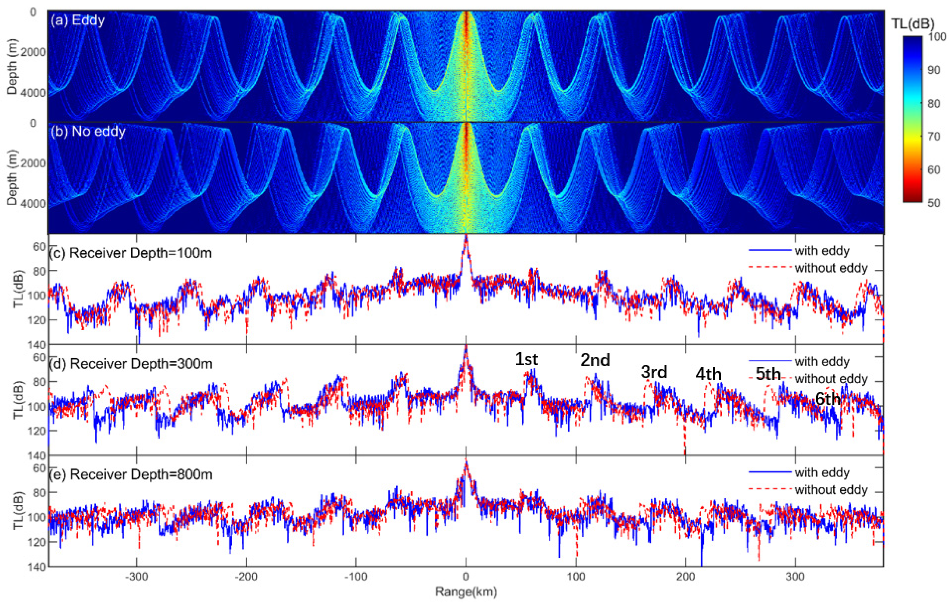
3.3. Propagation out of the Eddy
In the previous text, we have observed how the subsurface eddy affects acoustic propagation when the source is deployed at a distance from it. Now, we want to look at the changes when the source is deployed at the eddy center with sound rays propagating out of the eddy.
The differences in TL between the presence and absence of the eddy are shown in
Figure 8. Here, we still define the location of the sound source, i.e., the eddy center, as the range of zero. The subsurface eddy extends from −230 km to 230 km. We provide plots for the sequence of depths: 20 m, 100 m, 300 m, 460 m, and 800 m.
For a source deployed in the upper layer, above 100 m, only a slight shift of loss pattern is observed. As the source depth increases to 300 m, an intense pattern shift of convergence zones occurs, resulting in a 25 dB loss difference. These TL differences are again the result of the interaction between the acoustic signals and the intense temperature or sound speed gradient in the subsurface eddy. When the source depth exceeds 460 m, the subsurface eddy exhibits minimal impact on acoustic propagation.
In reference to
Figure 4, depicting the propagation of acoustic energy into the eddy from the neighboring water, a notable deviation in the loss pattern materializes when the source is positioned at approximately 100 m depth. Notably, a substantial dissimilarity between
Figure 4 and
Figure 8 is discernible, wherein the pronounced pattern shift of convergence zones in the latter instance transpires at a significantly greater source depth, around 300 m.
In particular,
Figure 9 illustrates further details of the intense TL pattern shift in
Figure 8c, where the source is placed at 300 m depth. With the fixed received depth of 100 m, TL curves in
Figure 9c show considerably good agreement, although the eddy case shows more loss (approximately 10 db) at some narrow range past 290 km. Therefore, the subsurface eddy has little effect at this depth.
With the fixed received depth of 300 m (
Figure 9d), the same depth as the sound source, we note again that a given convergence zone is plainly farther from the source with the presence of the eddy. There are six prominent convergence zones on the right side of the eddy. By comparing the TL curves under eddy-present and eddy-absent conditions, it can be found that the convergence zones in the eddy case exhibit a noticeable shift from the third convergence zone.
This feature is important in operating underwater sonar. For example, with a given figure of merit (90 dB), there is no overlap of the ensonified region between the eddy and no-eddy case at ranges past 150 km. In addition, compared with the unperturbed ocean environment, TL curves affected by the subsurface eddy is characterized by many small oscillations in the convergence zones compared with the unperturbed ocean environment. In
Figure 9e, with the fixed receiver depth of 800 m, the depth near the eddy bottom, the shift of TL curves is negligible.
4. Conclusions
In this study, we systematically explore the effects of a subsurface eddy on acoustic propagation. To the authors’ knowledge, this is the first study to present a detailed analysis of this aspect in the northwestern Pacific Ocean. The eddy with maximum speeds prevailing in the subsurface is about 460 km in diameter. The vertical size is more than 800 m. It drifted westward over 1500 km for eight months before being captured by the research cruise. Sound speed contours within the subsurface eddy display a biconvex lens shape. Sound speed changes of −4 m/s and 16 m/s are seen at constant depths of 100 m and 460 m, respectively, across the eddy. By utilizing a ray tracing model, we compared significant differences between scenarios with and without the subsurface eddy, effectively demonstrating its effects on sound propagation. Furthermore, we also examined the influence of variations in the depth and location of the sound source. The results revealed that subsurface eddies can lead to notable alterations, both in terms of quality and quantity, within the acoustic field.
For a shallow source located outside of the eddy, the subsurface eddy can affect sound propagation in the surface duct by altering the depth of the sonic layer. In contrast, no surface duct propagation occurs when the eddy is absent. When the source is deployed around 100 m depth, a given order of convergence zone tends to change its range and no longer overlap with that in the no-eddy case at ranges past 480 km. In the tenth convergence zone, the TL can exhibit variations of over 30 dB and shift their pattern range location by up to 14 km.
For a source located in the center of the eddy, the intense shift in convergence zone patterns described above was also observed, but it occurs only when the source is deployed around 300 m depth. The effects caused by the eddy become less noticeable when the source depth exceeds 460 m. Under optimum conditions, the existence of a subsurface eddy can decrease the propagation loss by 25 dB.
This finding indicates that subsurface eddies in the northwestern Pacific Ocean have a pronounced effect on sound propagation. The most ensonified region may be quite different from usual if a subsurface eddy occurs between a sound source and a receiver. The sound source could go undetected in the usual convergence zones, but the detection capability could be improved by choosing an optimal depth and range for the acoustic receiver. Future work will include quantifying the impacts on acoustic propagation caused by other physical oceanographic processes, like fronts, internal waves, and tides.


 ,
, 


