Numerical Simulation of the Unsteady Airwake of the Liaoning Carrier Based on the DDES Model Coupled with Overset Grid

Abstract

The wake behind an aircraft carrier under heavy wind condition is a key concern in ship design. The Chinese Liaoning ship’s upturned bow and the island on the deck could cause serious flow separation in the landing and take-off area. The flow separation induces strong velocity gradients and intense pulsations in the flow field. In addition, the sway of the aircraft carrier caused by waves could also intensify the flow separation. The complex flow field poses a significant risk to the shipboard aircraft take-off and landing operation. Therefore, accurately predicting the wake of an aircraft carrier during wave action motion is of great interest for design optimization and recovery aircraft control. In this research, the aerodynamic around an aircraft carrier (i.e., Liaoning) was analyzed using the computational fluid dynamics technique. The validity of two turbulence models was verified through comparison with the existing data from the literature. The upturned bow take-off deck and the right-hand island were the main areas where flow separation occurred. Delayed detached eddy simulation (DDES), which combines the advantages of LES and RANS, was adopted to capture the full-scale spatial and temporal flow information. The DDES was also coupled with the overset grid to calculate the flow field characteristics under the effect of hull sway. The downwash area at 15° starboard wind became shorter when the hull was stationary, while the upwash area and turbulence intensity increased. The respective characteristics of the wake flow field in the stationary and swaying state of the ship were investigated, and the flow separation showed a clear periodic when the ship was swaying. Comprehensive analysis of the time-dependent flow characteristic of the approach line for fixed-wing naval aircraft is also presented.

1. Introduction

Aircraft carriers are subject to atmospheric disturbances on the sea surface and the wake vortex field generated by their deck and deck superstructure. The disturbances could pose great challenges for the pilot during shipboard aircraft landings [1,2]. Meanwhile, the carrier itself is also subject to a six degree of freedom of movement during navigation against various wind directions, intensifying the flow separation and wake vortex flow structure. Numerous studies have been carried out investigating the characteristic of attachment layers, shear layers, and flow separation in this naval outflow field.

Earlier studies focused on utilizing simple frigate shape (SFS) where a series of wind tunnel experiments were carried out [3,4,5]. Helicopters are docked at the stern of these frigates, so the air disturbance above the stern apron is concerned. For the landing and taking off of fixed-wing aircraft carriers, the United States has the largest carrier battle group in the world. Polsky [6] and Shipman [7] studied the airwake flow structure induced by the CVN aircraft carrier. Kelly [8] used the CFD technique to predict the dynamic of wake on the UK’s new Queen Elizabeth Class (QEC) aircraft carrier. Compared to the CVN aircraft carriers, the QEC features double islands and an upturned deck structure, causing a more complex and unique wake structure. However, the study did not account for the more complex flow caused by the motion of the hull.

In essence, CFD has been widely adopted for capturing the wake of large vessels. The development of turbulence modelling has gradually transited from the Reynolds-averaged Navier–Stokes (RANS) models to the advanced large eddy simulation (LES). With the advancement in the turbulence model, more refined flow structures were also gradually revealed and resolved. In 2000, Reddy [3] first adopted the k-ε Reynolds time-averaged model to study frigate wake flow. The results showed a strong vortex zone in the helicopter landing area on the stern of the deck. Later, Polsky [9] used monotone integrated LES to study the air wake field on an LHA with a deck and island structure similar to aircraft carriers. The results showed the asymmetric flow field structure on the deck and noticeable upwash flow behind the island. Zhang [10] used LES to capture the high resolution of turbulence details in the flow field in a 1:100 scaled model with a 20 million grid mesh. Bi-stable behavior behind the ship was clearly shown in their result.

For larger vessels, using the ship’s side width as the characteristic length, the Reynolds number is typically between 10⁴ and 10⁷ orders of magnitude. At high Reynolds numbers (i.e., above 10⁴), the three-dimensional unsteady flow is characterized by fully developed turbulent flow. Previous studies have demonstrated that flow separation in a bluff body (including vessel) is independent of Reynolds number above 10⁴ [11,12]. Based on this, large vessels can be carried out in a scaled-down model in wind tunnel experiments and CFD methods. The RANS model is suitable for simulating high Reynolds number flow field, benefiting from its robustness and saving of computational resources. Nevertheless, it fails to handle the strong flow separation from bluff bodies [13,14].

Due to the dimensionless boundary layer thickness and high-resolution meshes required by the LES, simulating a full-size model demands an huge amount of computational resources. On the other hand, RANS smears out the effects and shear stresses due to turbulent fluctuations. Detached-eddy simulation (DES), a method combining the advantages of both LES and RANS [15,16], could be a better candidate to resolve the bluff body bypass flows at a high Reynolds number. The DES adopts RANS for attached flows near the wall while using LES for separated flows far from the wall. As a result, DES could significantly reduce the required grid resolution, in particular at the near wall regions. This model is suitable for the numerical calculation of the air flow field in the wake of a ship [17,18].

Forrest and Owen [19] used the DES model to investigate the SFS2’s airwake under the influence of different wind angles. Watson [20] studied the QEC carrier’s wake characteristics using both scaled-down and full-scale models using the water tunnel experiment and DES turbulence modeling. Their study successfully captured the dynamics of the aft-side wake of the carrier (particularly the airflow disturbances on the aircraft approach line) with reduced computational effort compared to the LES model. Recently, Owen [21] presented a PIV measurement for the stern flow field in the ship under three degrees of freedom of motion in pitch and roll. The DES SST k-ω turbulence model was also adopted to simulate the spatial flow field around the ship when it is stationary. Nisham [22] also adopted the DES model to investigate the effect of ship motion on the airflow behind the deck superstructure. The flow field was found to be significantly disturbed by the change in the period of the ship’s motion.

Improved versions of the delayed detached-eddy simulation (DDES) and improved delayed detached-eddy simulation (IDDES) have been commonly employed for studies on airwake [20,23,24]. The DDES model incorporates a delay factor that enhances the ability of the model to distinguish between LES and RANS regions on meshes where spatial refinement could give rise to ambiguous behavior. For IDDES, the subgrid length-scale includes a dependence on the wall distance. The authors claim that the DDES results present more realistic 3D features, and agreement on the experimental data is good. The authors recommended DDES modeling for reliable wake prediction [25,26].

Although research has been carried out investigating the naval wake, most studies have focused on frigates and destroyers. The Liaoning ship features a relatively distinctive large island and upturned deck. The airwake field under the influence of the superstructure and the conditions of sway has not been well understood. This research presents a comprehensive investigation of the airwake on the upturned deck, superstructure area, and the approach line of the Liaoning ship. Attention is also directed to study the effects of sailing in combination with wind angles, as well as hull swaying on the wake flow structure. Turbulence fluctuation of the transient flow field in the stern is provided for the aircraft recovery process.

DDES simulations were carried out based on a scaled-down aircraft carrier model. The purpose of using the scaled-down model was to verify the accuracy of the mathematical model and to predict the model wake vortex distribution. Furthermore, aiming to capture the realistic flow field state during navigation, the DDES turbulence model was also coupled with the overset dynamic grid to resolve the wake structure for a full-scale model. Variations of carrier wake under different wind angles and hull swaying conditions were also analyzed. This study incorporated hull heave motion, which complicates the airflow in the aft region and intensifies disturbances during aircraft landing. This motion also challenges precise positioning, making the scenario more reflective of actual operation.

2. Numerical Method

This study adopted DDES to simulate the wake flow field of an aircraft carrier under different wind directions. The focus is on the flow field information on the descent line of a fixed-wing carrier aircraft. The aircraft carrier speed is typically 30 knots; therefore, the air can be considered as an incompressible fluid. We investigated the structure of the carrier wake field by using a scaled-down model and verified the accuracy of the numerical model. The model was then scaled up to a full-scale model to investigate the changes in wake flow caused by the swaying of the carrier during navigation. All the computations presented in this study were performed using a three-dimensional finite-volume unstructured solver (STAR CCM).

2.1. DDES (Delayed Detached Eddy Simulation) Model

The strict mesh requirements of LES pose significant challenges in resolving a full-size model. The DES model combining the advantages of both LES with RANS models was therefore adopted. The DES uses the SST k-ω turbulence model [27] near the wall, and the free shear flow far from the wall is treated with the LES model. This method allows for a simple and efficient transition from the RANS to the LES model, capable for a full-size simulation with the length scale of several hundred meters in magnitude. In addition, it is a challenging task to generate good-quality mesh near the wall regions due to the complex vessel structure. An improved model of DES, DDES, was therefore adopted in this study. DDES defines a more general form of grid scale combined with the distance from the wall [16].

The governing equation of SST DDES model is as follows:

$${\displaystyle \frac{\partial \left(\rho k\right)}{\partial t}}+{\displaystyle \frac{\partial \left(\rho u_{j}k\right)}{\partial u_j}}=P_k-\rho {\displaystyle \frac{k^{3/2}}{l_{DDES}}}+{\displaystyle \frac{\partial }{\partial x_j}}\left[\left(\mu +{\displaystyle \frac{{\mu }_t}{{\sigma }_k}}\right){\displaystyle \frac{\partial k}{\partial x_j}}\right]$$

(1)

$${\displaystyle \frac{\partial \left(\rho \omega \right)}{\partial t}}+{\displaystyle \frac{\partial \left(\rho u_j\omega \right)}{\partial u_j}}={\displaystyle \frac{\partial }{\partial x_j}}\left[\left(\mu +{\displaystyle \frac{{\mu }_t}{{\sigma }_{\omega }}}\right){\displaystyle \frac{\partial \omega }{\partial x_j}}\right]+2\left(1-F_1\right){\displaystyle \frac{{\sigma }_{\omega 2}\rho }{\omega }}{\displaystyle \frac{\partial k}{\partial x_j}}{\displaystyle \frac{\partial \omega }{\partial x_j}}+\alpha {\displaystyle \frac{\rho }{{\mu }_t}}{P}_k-\beta \rho {\omega }^2$$

(2)

where k is the turbulent kinetic energy; ω is the specific dissipation rate; ρ is the density; u_j is the velocity component; x_j is the spatial coordinate component; μ is the dynamic viscosity; σ_k and σ_ε are model constants used to control unsteadiness; P_k is the production of turbulent kinetic energy; and μ_t is the turbulent viscosity.

$${\mu }_t=\rho {\displaystyle \frac{a_{1}k}{\max \left(a_1\omega ,F_{2}S\right)}}$$

(3)

where F₁ and F₂ are blending functions.

The DDES length scale in Equations (1) and (2) is as follows:

$$l_{DDES}=l_{RANS}-f_d\max \left(0,l_{RANS}-l_{LES}\right)$$

(4)

$$l_{RANS}={\displaystyle \frac{\sqrt{k}}{C_{\mu }\omega }}$$

(5)

$$l_{LES}=C_{DDES}\Delta$$

(6)

$$C_{DES}=C_{DES,k-\omega }{F}_1+C_{DES,k-\epsilon }\left(1-F_1\right)$$

(7)

The blending function f_d in Equation (4) is written with the following relations:

$$f_d=1-\tanh [{(C_{d1}{r}_d)}^{C_{d2}}]$$

(8)

$$r_d={\displaystyle \frac{{\nu }_t+\nu }{{\kappa }^2{y}^2\sqrt{0.5(S^2+{\Omega }^2)}}}$$

(9)

where S is the magnitude of the strain rate tensor and Ω is the vorticity tensor, where the coefficients are as follows [28]:

C_d1 = 20, C_d2 = 3, κ = 0.41, C_DES,k-ω = 0.78, C_DES,k-ε = 0.61.

By introducing a delay function f_d, DDES ensures the continued use of the RANS model within the boundary layer, avoiding errors caused by grid transitions. The model is suitable for simulating the complex geometry of aircraft carriers and high Reynolds number flows, particularly in accurately handling boundary layers and flow separation.

2.2. Overset Grid

The overset mesh technique is more suitable for modeling the spatial motion of a rigid body in comparison to the dynamic deformation mesh approach. This approach eliminates the process of reconfiguring the topology of the mesh during motion. In simulating the object motion, the entire computational domain is divided into two parts: a background mesh and a motion mesh. The two separate meshes are discretized for the respective solution domains. The transfer of field information between the two sets of meshes is carried out by interpolation [29,30]. When describing the ship’s sway motion, the coordinates of the background domain are set to be stationary with respect to the earth, while the grid around the ship is equated to the ship’s sway, with the grid in the motion domain remaining unchanged.

2.3. Post-Process

2.3.1. Q-Criterion

Q-criterion is highly effective in capturing vortices, particularly in turbulent flows. It is frequently used for flow field visualization to provide a clear depiction of vortical structures. To identify the order structure of the turbulent field of the carrier wake vortex, the Q-criterion is employed to describe the vorticity. Q is the second invariant of the velocity gradient tensor [31].

$$Q={\displaystyle \frac{1}{2}}({‖\Omega ‖}^2-{‖S‖}^2)$$

(10)

where Ω is the velocity gradient inverse symmetry tensor and S is the velocity gradient symmetry tensor. When Q is in a positive value, the pressure field exhibits a low-pressure region at the center surrounded by a high-pressure value. A positive threshold Q-equivalent surface was chosen to identify the sequential vortex structure.

2.3.2. Turbulence Intensity

In this study, turbulence intensity (Ti) was used to quantify the pulsation of the wake under different conditions. Ti is defined as the root mean square of the turbulent velocity fluctuations divided by the fluid velocity at the far field, which is given as follows:

$$Ti={\displaystyle \frac{\sqrt{\frac{1}{3}\left(u^{\prime }+v^{\prime }+w^{\prime }\right)}}{U_{\infty }}}$$

(11)

where $u^{\prime },v^{\prime },w^{\prime }$ are the pulsation values of each velocity component, and U_∞ is the free-flow velocity.

3. Numerical Calculations for the Aircraft Carrier

3.1. Geometry Model

The aircraft carrier model refers to the full-size dimension of the Liaoning ship. The geometric model and feature dimensions are shown in Figure 1. The hull, deck, and complex structures on the ship were simplified for the ease of mesh generation. An asymmetrical air wake could be generated despite having a symmetric superstructure [32]. The asymmetrical superstructure of an aircraft carrier with the island on the right side of the deck creates irregular airflow disturbances, further exacerbating the asymmetry airflow structures. Furthermore, the aircraft carrier has a bow deck for slip take-off incur flow separation. Thus, the simplified model retains most of the key features of the island and the upturned deck.

A Cartesian coordinate system was established with the x-axis parallel to the direction of the traveling ship. The y-axis and z-axis were orthogonal to the gravitational acceleration and horizontal sea level, respectively. The left rear edge of the deck was marked as the origin of the coordinate system. Numerous studies have verified the accuracy of the numerical simulations by comparing them with the wind tunnel experimental results of the scaled-down model. Greenwell [33] and Healey [34] verified that the flow field characteristics of flow separation as a fluid flows through a bluff body are independent of the Reynolds number. It is therefore possible to use the DDES algorithm to resolve the flow field in the context of the scaled-down model. A reduced scale model (i.e., 1:100) was used in this study.

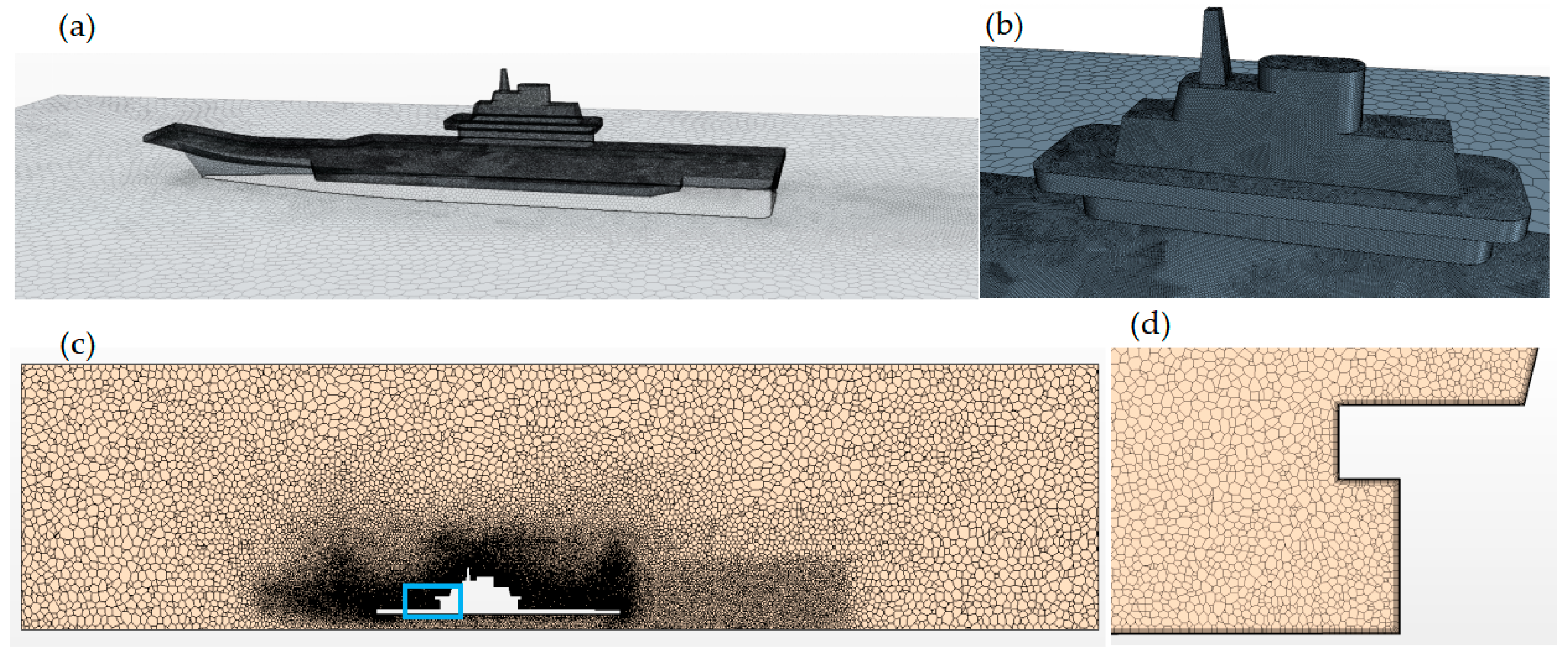
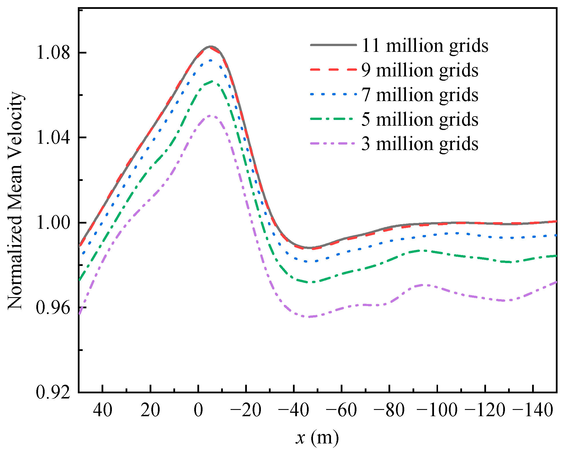
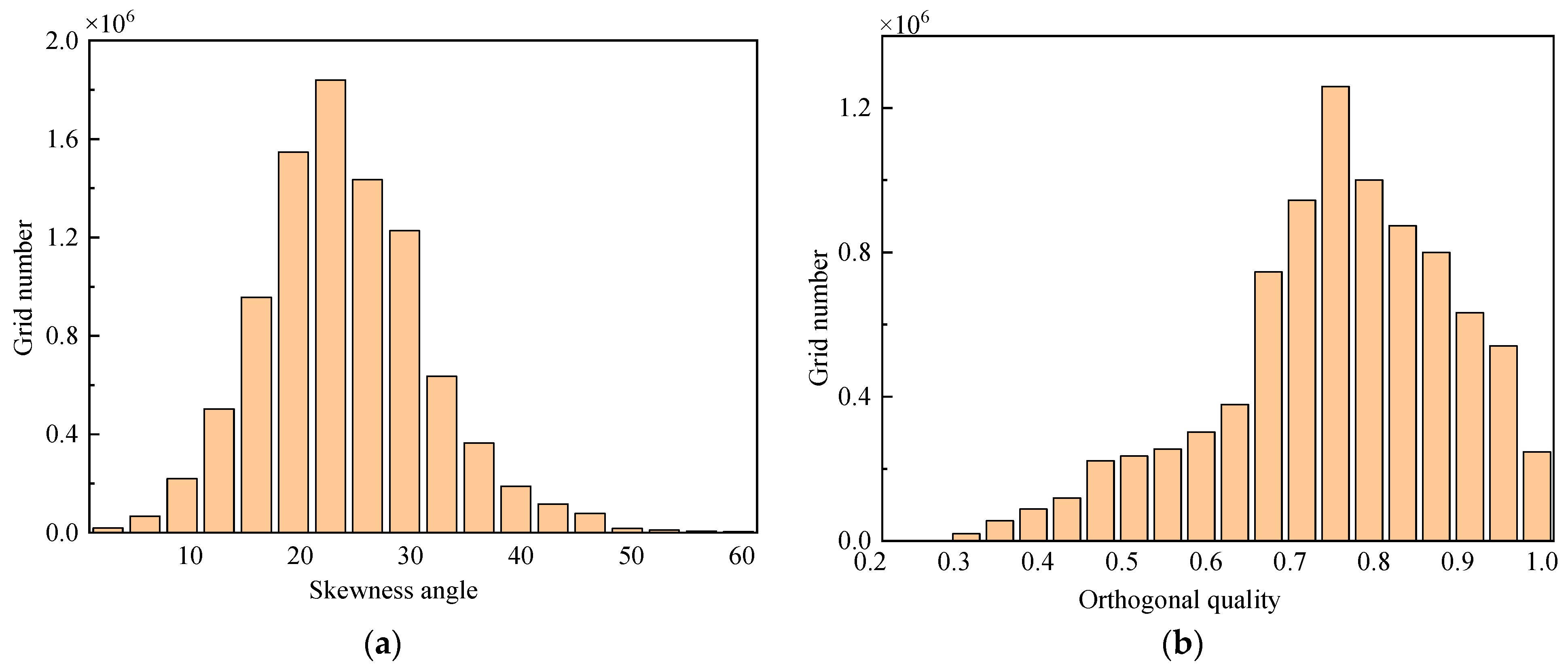
3.2. Mesh Gridding

Due to the irregular shape of the carrier hull, a more adaptable polyhedral mesh was used. This type of grid has a low number of grid nodes and high grid quality for the same size conditions. The upturned deck and the island play a vital role in generating the airwake. The approach line of the aircraft must pass through the wake area. High-resolution grid meshes were generated in these sections to capture the airwake. Figure 2 shows the schematic diagram of the aircraft carrier model grid. At the wall region of the scaled-down model, the dimensionless thickness of the wall surface y+ was kept below 1. The growth rate of the boundary layer grid thickness was of 1.2 [20].

The velocity along the aircraft carrier’s approach line was used as the validation criterion, as shown in Figure 3. According to the grid-independence validation, grids consisting of 9 million cells were employed. The boundary layer grid thickness was 0.5 m, with 12 layers. The near-wall grid size was 0.1 m, and the grid growth rate was 1.2. The grid quality was assessed using the skewness angle and orthogonal quality, as shown in Figure 4. The mesh skewness was below 60°. The grid orthogonality quality exceeded 0.2, meeting the required mesh quality standards.

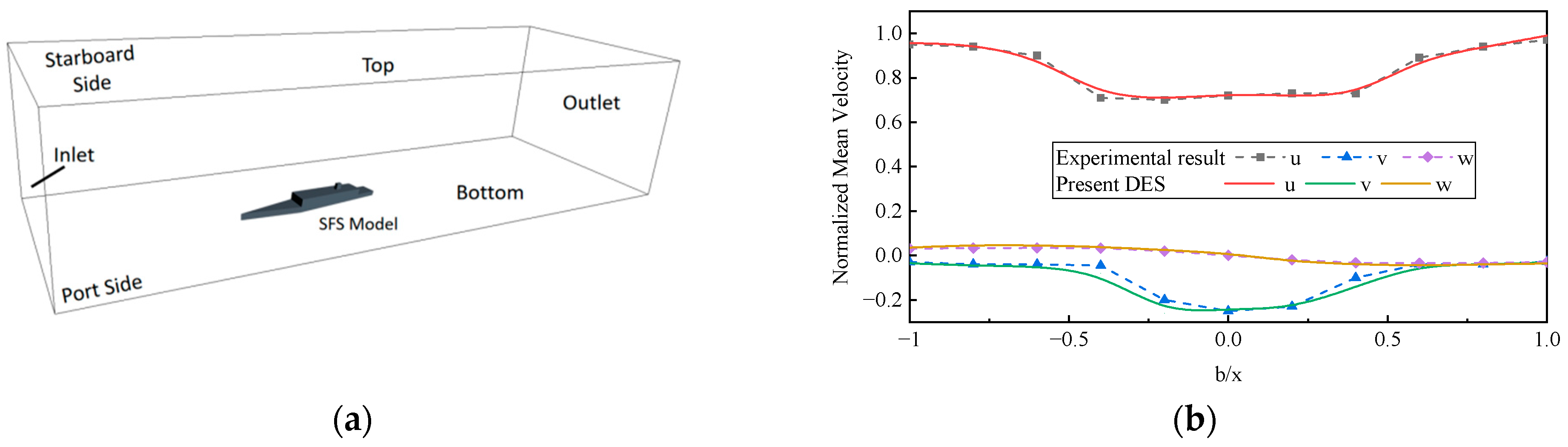
3.3. Boundary Conditions

The boundary conditions and the range of computational domains are shown in Figure 5. The computational domain had a length of four times the ship length, a width of five times the ship width, and a height of five times the ship height. This article used the relative velocity approach to model the carrier’s sailing speed, with the air flowing at the same speed as the sea. The lower surface of the computational domain represents the sea level.

Relative wind speed was used in place of ship speed. Air and sea water were relatively static with no slip between them. It was assumed that the seawater flow was unaffected by the hull and that the water surface was wave-free. The assumption of a stationary sea surface was made to focus on the effects of the ship’s pitch motion on the wake field, facilitating a clear comparison between a stationary and a moving hull. Large waves were not present in conditions suitable for aircraft operations. The sea surface fluctuations were comparable in magnitude to ship motion, and the influence of sea surface waves can be considered negligible. Furthermore, since the sea surface was 17 m below the flight deck and the approach line was situated above the deck, the impact of sea surface fluctuations on the approach line was minimal. Therefore, the bottom of the computational domain was modeled as a slip wall. No-slip wall condition was specified at all surfaces of the hull. For the scaled-down model, the air velocity at inlet was set as a uniform 1.0 m/s.

For the full-scale model, the inlet velocity was 15.4 m/s, which is equal to the sailing speed. Outlet boundary was specified as Neumann boundary condition, $\partial {\overline{u}}_i/\partial x_i=0$. The upper, left, and right boundaries were assumed as a symmetrical boundary [10]. The top was $\partial \overline{u}/\partial y=\partial \overline{w}/\partial y=0$, $\overline{v}=0$. The left and right boundaries were $\partial \overline{u}/\partial z=\partial \overline{v}/\partial z=0$, $\overline{w}=0$.

The Reynolds number of the flow was approximately 10⁷, with the hull width taken as the characteristic length. When the fluid flows passed the whole a ship length, the flow field characteristics were assumed to be well-established. The results of the simulation were captured starting from this time.

4. Results and Discussion

4.1. Numerical Methods Validation

Model validation is crucial for any numerical simulation to ensure the reliability of the model predictions. For the Liaoning aircraft carrier, unfortunately, there is a lack of actual experimental data, and very little information is available in the literature. In this study, the SFS-type ship was also constructed as a benchmark model comparing the DDES model predictions with existing data from the literature. The dimensionless positions x/L_ship = 0.5 and y/H_ship = 1 were chosen for data comparison (L_ship and H_ship mean the length and height of the SFS, respectively.). As depicted in Figure 6, the DDES model predictions were in excellent agreement with the corresponding experimental data [13]. The same mathematical model was transferred to the Liaoning aircraft carrier for numerical simulation. The grid-independent study was also performed, ensuring the reliability of the mathematical solution in this study.

4.2. DDES Scaled-Down Model Results

This research considers the effect of wake vortices generated by the carrier structure on the return of the carrier aircraft during the landing process, focusing on the area of space above the deck level. Figure 7 shows the instantaneous isosurface of the Q-criterion value for the headwind flow over aircraft carrier model. On the deck and the leading edge of the island, the air was squeezed at speeds increasing to over 2 m/s. The diagram shows that the air formed a strong flow separation around the hull. The angle of descent of a typical fixed-wing aircraft (i.e., the line of trajectory) makes an angle of 3° with the horizontal during aircraft recovery. It is worth noting that the modern F35 fighting jet lands with a relatively steeper approach line at the 7° angle. This downstream line all goes through the airwake influence area. The figure shows the significant disturbance of the flow field on the approach line of the aircraft.

Figure 8 shows the velocity magnitude and its corresponding vertical velocity component distribution over the central section of the island. There were low-speed zones aft of the island and above the aft edge of the deck. Significant velocity fluctuations with high-velocity gradients can be observed in this region. From the vertical velocity component, the wake went through downwash and upwash backwards at the aft edge of the deck.

The above vorticity and velocity distributions show the overall flow characteristics of the carrier wake at a macro level. Attention is now directed to the change in velocity magnitude on the ship’s flight path. Figure 9 illustrates the instantaneous air velocity distribution along the aircraft’s approach line when the aft edge of the deck was set as the original point (i.e., 0) in the normalized x-axis. To be consistent with the coordinate system, the right-hand side of the horizontal coordinate was set as negative. The leftmost side was the touchdown point for the landing of the aircraft. As depicted, the overall trend of velocity was relatively smooth above the deck. Nonetheless, once it passed the trailing edge of the deck, the speed started to decrease and fluctuate rapidly. For the landing process, the vertical velocity component had the most direct impact on the aircraft control and should therefore receive attention. From the vertical velocity component, an average curve indicates that a clear region of downwash appeared after passing the aft edge of the deck. However, an instantaneous curve shows local fluctuations were also observed within the downwash area. After 0.5 ship lengths, the downwash airflow started to diminish and returned to a horizontal state.

4.3. Full-Size DDES Numerical Study

As mentioned before, a full-size DDES simulation was carried out to study the impact of different sailing angles and hull sway on aircraft carriers in moderate sea conditions. In the full-scale simulation, the dimensionless first grid layer on the surface (i.e., y+) was less than 30 with an exponential growth law. Grid resolution for the stern area of the airwake section was further refined to capture the details of the flow field. Wake refinement was employed. The grid size in the core area of the hull was less than 0.3 m. In the wake area behind the deck within 200 m, the grid size was less than 1 m. In other areas, the grid size was less than 3 m. This method ensures the accuracy of the study and saves a large number of grids.

A previous study suggests that ocean wind speeds are consistent with the marine atmospheric boundary layer Equation (12) [35].

$$V=V_{\mathrm{r}}({\displaystyle \frac{\ln (y/y_0)}{\ln (y_{\mathrm{r}}/y_0)}})$$

(12)

The above equation indicates a greater variation in velocity close to sea level. The deck level of the aircraft carrier studied in this research was of 17 m above the sea level. At this range, the speed variation was relatively insignificant. Furthermore, the focus of this investigation was on the variation of the velocity field above the deck due to the influence of the superstructure. Therefore, a uniform inlet velocity profile was used in this investigation. A uniform air speed of 15.43 m/s was initialized across the domain with a time step of 0.01 s. Numerical results began to be extracted when the initial wake of the superstructure flowed over a ship length.

In practice, aircraft carriers often sail head-on into the wind direction, aiming to reduce chances of having side wind and the relative speed of the aircraft to the ship during landing. On the other hand, sidewinds are inevitably encountered. The simulation results from the scaled-down model mentioned above show that the wake vortex behind the island caused strong airflow disturbances. When the carrier was sailing with a 15° starboard wind, the island’s airwake swept over the carrier’s approach line, posing the most significant effect on the landing process. The variation of airwake and velocity fluctuations along the approach line over time are considered in this section when the carrier was faced with headwind and green 15° wind.

Figure 10 compares instantaneous Q-criterion contour distributions at headwind and green 15° wind. The model predicted the flow separation from the deck area as well as from the ship’s island. Due to the upturned deck, the airwake separating from the bow ran directly through the entire carrier. Nevertheless, the airwake from the bow flowed directly off the port side of the deck at green 15° wind. The separation vortex pathed the entire descent line of the final recovery phase.

Figure 11 shows the velocity distribution in the cross-section of the carrier island. Similar to the result shown in Figure 8, velocity pulsations and downwash areas were also clearly observed behind the island.

Figure 12 compares the development of the flow line above the passing deck at 0° to windward and 15° to starboard. It shows that the flow line was generally smooth at headwind, with a local recirculation forming behind the island. Downwash flow formed at the rear side of the deck.

The airflow around the island formed a rapid downwash with green 15° wind on the starboard side. The left-hand streamline of the deck continued down past the aft edge of the deck. The right-hand side of the deck flowed past the aft edge of the deck, quickly turning into an upwash. When the carrier was sailing with a starboard wind, the tendency to wash down or wash up at the aft edge of the deck was more pronounced. The airflow exhibited a downwash on the left and an upward wash on the right. This introduced significant disturbance to the landing procedure of the ship’s aircraft.

Figure 13 compares the instantaneous velocity and vertical velocity component along the last 200 m of the approach line during the recovery. The x-axis in the graph was defined the same as in Figure 5. The touchdown point of the aircraft was 50 m from the stern of the ship. As depicted, the overall velocity magnitude for the green 15° wind case was lower in comparison with the headwind case (i.e., 0°); however, the overall velocity fluctuation was greater than the headwind case.

For the vertical velocity component, the average curves in Figure 13c reflect the regions of downwash and upwash along the approach line. The air flow abruptly descended after passing the aft edge and returned to horizontal after 70 m. An instantaneous curve showed that the vertical velocity above the deck was relatively smooth for the headwind. When the carrier was sailing with a green 15° wind, the vertical velocity component started to fluctuate above the deck. The length of the downwash area behind the stern was relatively shorter than the headwind case. However, a clear upwash airflow appeared as it continued traveling towards the aft. The magnitude of the upward velocity reached 3 m/s. A series of test lines with 100 m spacing were selected for the descent line of the ship. The velocity distribution along the altitude direction is compared.

Figure 14 shows the velocity distribution on the selected test lines. As depicted, for most of the line locations, the velocity magnitude for the headwind case was greater than that for green 15° wind at the same height. In terms of vertical velocity components, a downwash flow was formed near the island at the aft edge of the deck. For the green 15° wind case, there was a rapid shift to an upward wash with a greater upward speed. The change of lift force that the aircraft will face in this situation requires more demanding control manipulations.

Figure 15 shows the distribution of turbulence intensity in the approach line cross-section. As shown in the figure, the superstructure significantly intensified the wake turbulence. The increase in turbulence intensity occurred in the landing area at green 15° wind conditions.

It is worth noting that the instantaneous flow field did not reflect the change of the flow field with time. Therefore, the variation of the airwake on the approach line with time should receive more attention. Figure 15 shows the five probe points on the approach line. Here, the touchdown point was set to point 1. Sequential probe points were then taken for every 50 m along the x-direction of the approach line. Point 1 was on the deck surface and Point 2 was too close to the deck. The vertical component of the velocity of the two points varied very little. Therefore, they were not included in the discussion. Figure 16 shows the time history of the instantaneous velocity variation along the approach line. The graph records the variation of the vertical component of the velocity with time at three points.

Figure 17 records the vertical velocity fluctuation at Points 3, 4, and 5 with time. As depicted, the vertical component at these three points was flowing upwards most of the time, posing a significant difference to the downwash flow at headwind. At Point 3 and 4, the upward velocities had a greater magnitude compared to Point 5. As evidenced by the Q-Criterion contour, as well as the streamline diagram, the airflow at these three locations was the forward flow through the island. This indicates the rapid formation of upwash flow from the stern stream under the influence of the carrier island. In this case, the downwash area was shorter, and the upwash was more intense.

4.4. Effects of Hull Motion on Airwake

Figure 18 shows the background grids and the motions grids. The interpolated grid regions are merged into a single entity. Six-degree freedom of motion of the hull can be caused by wind and waves in the sea. It is challenging to model this motion accurately. The components of motion can be described by the simple harmonic motion. The amplitude and angular frequency are related to sea state, hull size, and displacement. When travelling at 30 knots in moderate sea conditions, the carrier produced a heave and pitch of approximately 2 m and 1°. Movement patterns are documented in a study by the US Navy (AD-7435209). Heave motion h_m is written as follows:

$$h_{\mathrm{m}}=1.22\sin (0.6t)+0.3\sin (0.23t)$$

(13)

The hull motion is described using the overset mesh method. The foreground grid covers the entire hull. Equation (13) describes the displacement of the ship’s pitch motion, including the relationship between displacement and time. This equation was set as a custom field function and assigned to the aircraft carrier’s hull region. During the computation, the carrier’s region moved according to the position–time relationship specified by the equation. Interpolation calculations were performed between the carrier’s boundary and the background mesh, with a grid size difference at the intersection not exceeding 3.5 times to ensure accurate computation. As the carrier’s boundary continuously changes position during motion, two sets of meshes within this range must be defined in terms of size during mesh generation, ensuring that the mesh meets computational requirements.

4.4.1. Headwind with Heave

Figure 19 shows the Q-criterion contour plot for a carrier in headwind sway with heave motion according to Equation (13). As depicted, the stern vortex was more abundant compared to the stationary hull (see Figure 10) and extended for a longer distance behind the ship. When the ship was stationary, these flow separations occurred mainly at the island and on the forward side of the deck. When the ship was swaying, in addition to flow separation at the leading edge of the deck, flow separation also occurred at the trailing edge of the deck. Furthermore, the diagram also shows that the separating vortex at the rear of the deck had a periodic behavior.

Figure 20 records the variation of vertical velocity component over time at probe points under the headwind sway condition. The figure indicates that the vertical velocity component at these points clearly exhibited periodic fluctuations. The amplitude of the fluctuation was higher compared to the stationary situation. The wave peaks passed downwards in spatial and temporal sequence in the order of the points, with the amplitude decreasing in turn. Point 3 mostly fluctuated between −3 and 6 m/s. Points 4 and 5 mostly fluctuated between −1 and 4 m/s, with the upward direction accounting for a much greater proportion than the downward direction. The fluctuating effects transmitted to more distant positions than that in the stationary hull case above.

4.4.2. Green 15° with Heave Motion

Figure 21 shows an isosurface plot of the airwake Q-criterion for a green 15° wind swaying condition. The airwake separating from the island passed through the touchdown point area. In contrast to the stationary hull, additional periodic separating vortices behind the aft deck were generated, together with the long straight-shaped airwake. This periodic flow separation could aggravate the pilot workload.

Figure 22 records t records the variation of vertical velocity component over time at probe points along the approach line under the green 15° wind swaying condition. The figure shows that Point 3 (i.e., 50 m from the aft edge of the deck) exhibited more significant periodic fluctuations. The amplitude of fluctuation diminished at Point 4 yet remained periodic. The vertical velocity at Point 5 fluctuated around 0 to 0.7 m/s, indicating that locations closer to the deck edge were more strongly disturbed in the crosswind condition. The influence of the airwake at the approach area (i.e., 150 m away from the aft edge) was diminished.

The power spectral density (PSD) plot is often used to identify frequencies in non-unsteady signals containing most of the energy. Figure 23 shows the comparison of spectral analysis of vertical velocity fluctuations over Point 3 in between stationary and moving states. The power density in the motion state was significantly higher than it was at the hull static state. The frequency at the maximum power occurred at 0.1 Hz, which coincided with the ship heave frequency.

Figure 24, Figure 25 and Figure 26 show the distribution of turbulence intensity along the approach line. The variation in turbulence intensity due to the angle of the wind can be seen in the graph. The swaying of the hull itself also caused an amplified turbulence intensity compared to that shown in Figure 15. In particular, when the ship was swaying, from the aft edge of the deck to 50 m behind the deck and in the height range 0 to 15 m, it caused stronger turbulence intensity. This range was the critical path of the final recovery of the ship’s aircraft.

5. Conclusions

In this study, the numerical model employed DDES, and the mesh used polyhedral grids adapted for complex structures. This approach enabled the detailed analysis of the spatial flow field around large objects. A scaled-down model was constructed to verify the accuracy of DDES. The numerical results were in good agreement with the literature. The ship was characterized by an upturned bow deck and an island on the right-hand deck. These protruding structures can cause flow separation and velocity fluctuations in the wake field, posing challenges to the landing process of a shipboard aircraft. The sway of the hull also intensified the fluctuations in the wake field. In order to gain more insight into the fluctuations of the LN wake, this research used DDES coupled with the overset grid method to describe the dynamics airwake of the moving hull. The combination of custom field functions and overset grids enabled control of movement within the spatial domain of large objects. The detailed conclusions are summarized as follows:

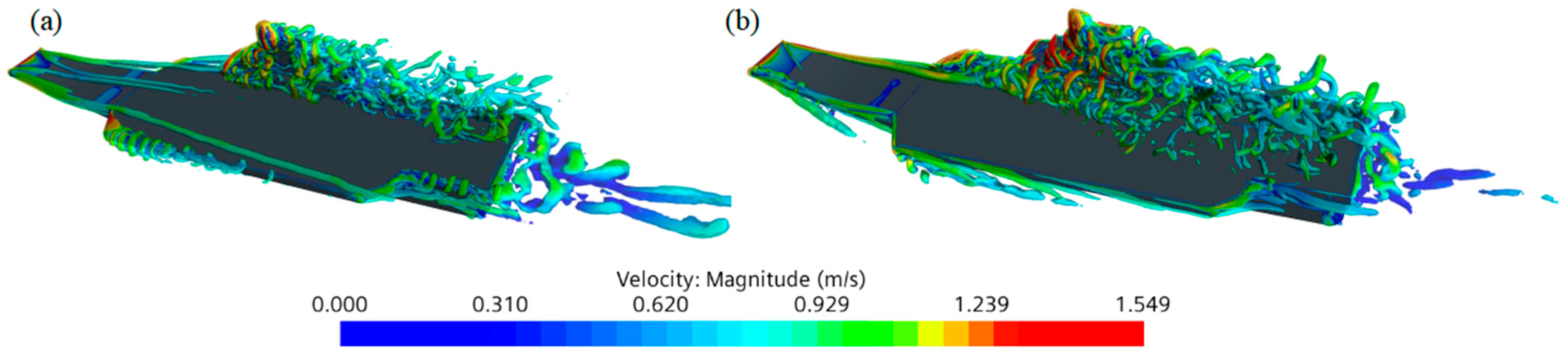
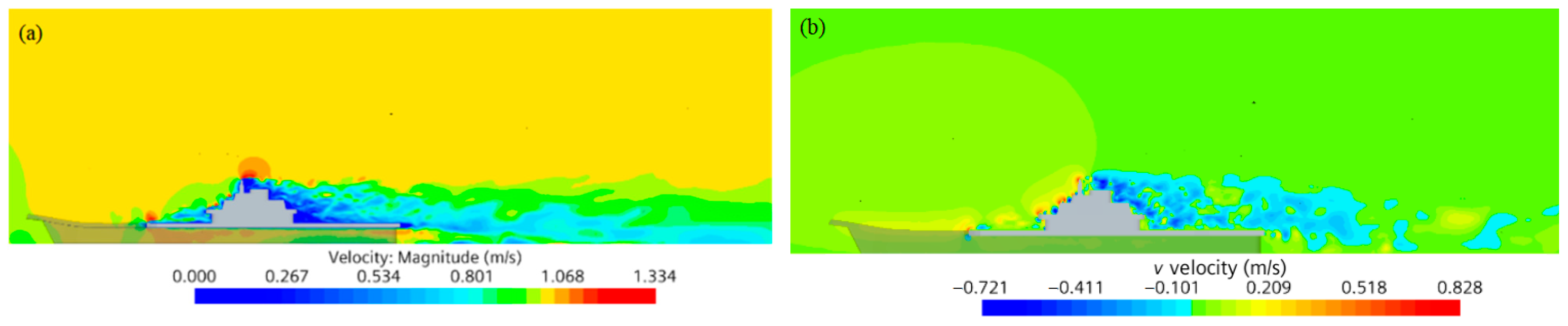
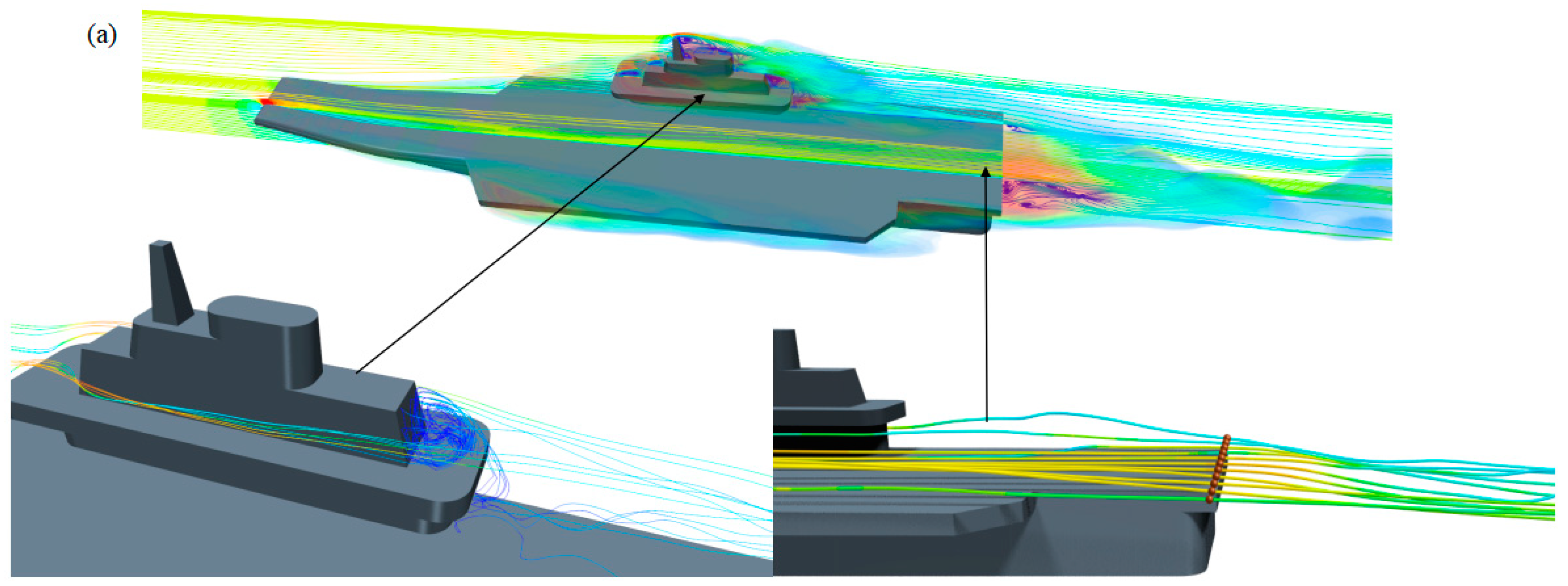
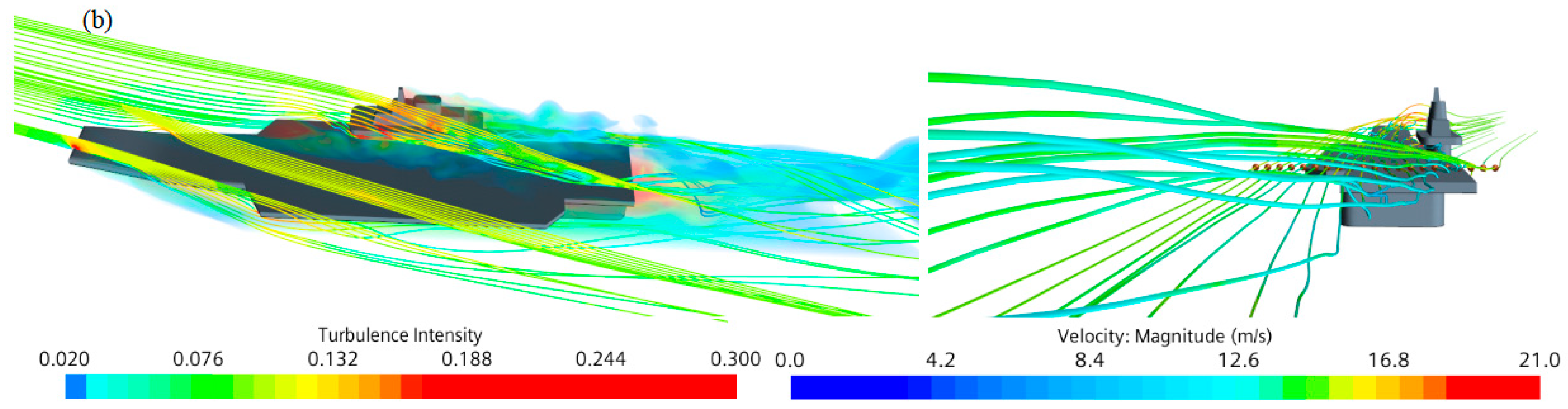
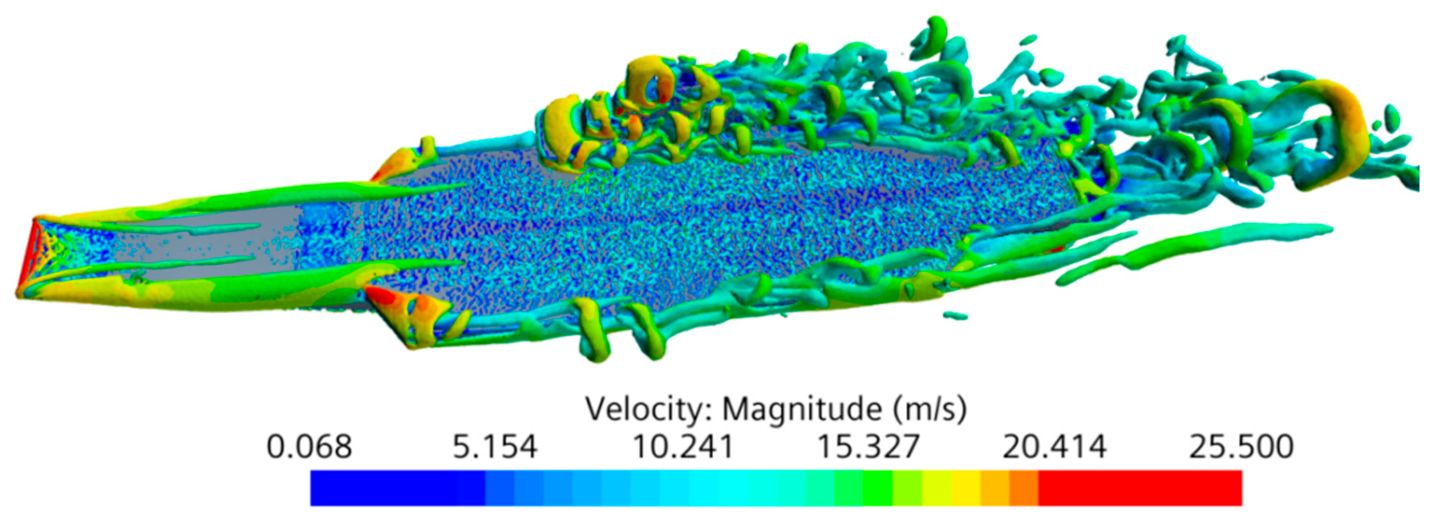
• The DDES method was employed to simulate the airwake of the carrier hull under the stationary condition using a scaled model. Flow separation was found to occur mainly at the upturned bow deck, the forward edge, and the protruding island. A clear downwash area appeared after passing the aft edge of the deck.
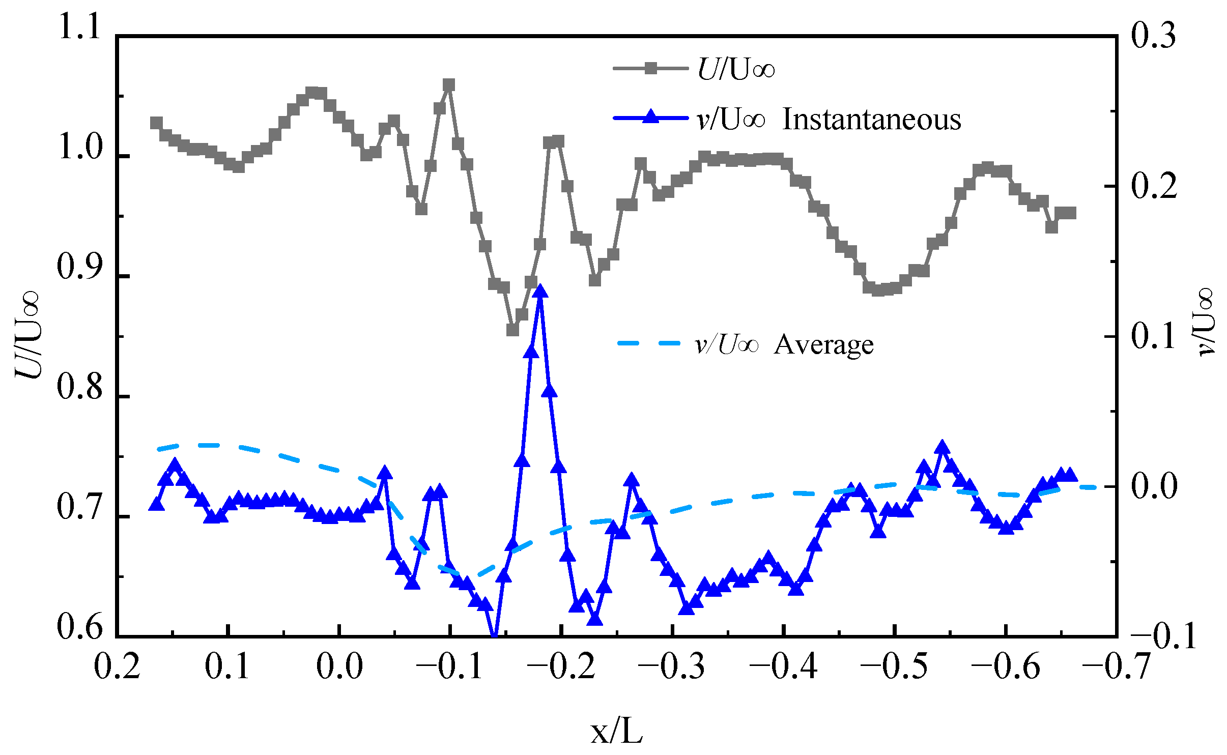
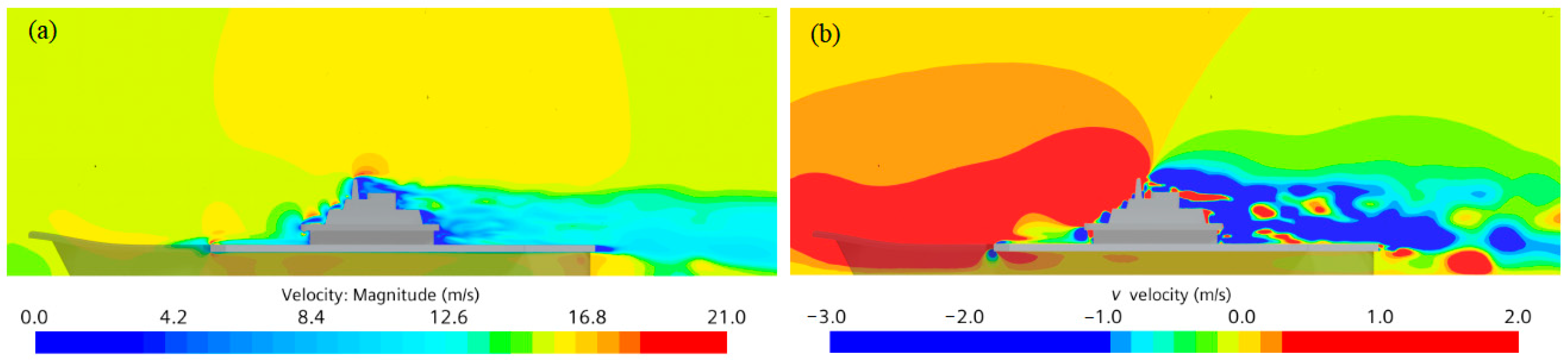
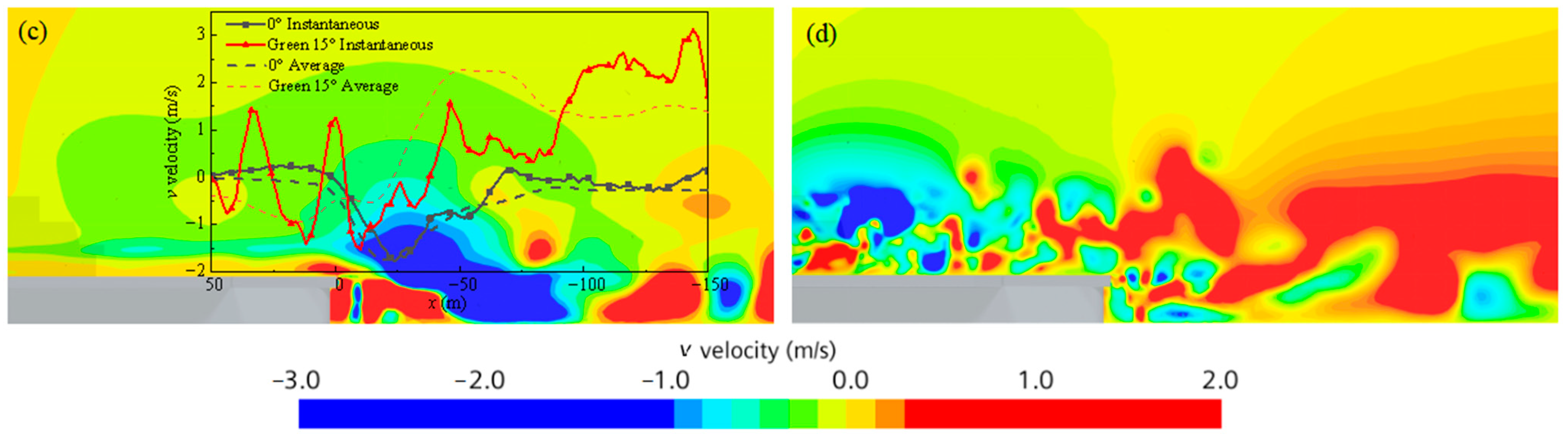
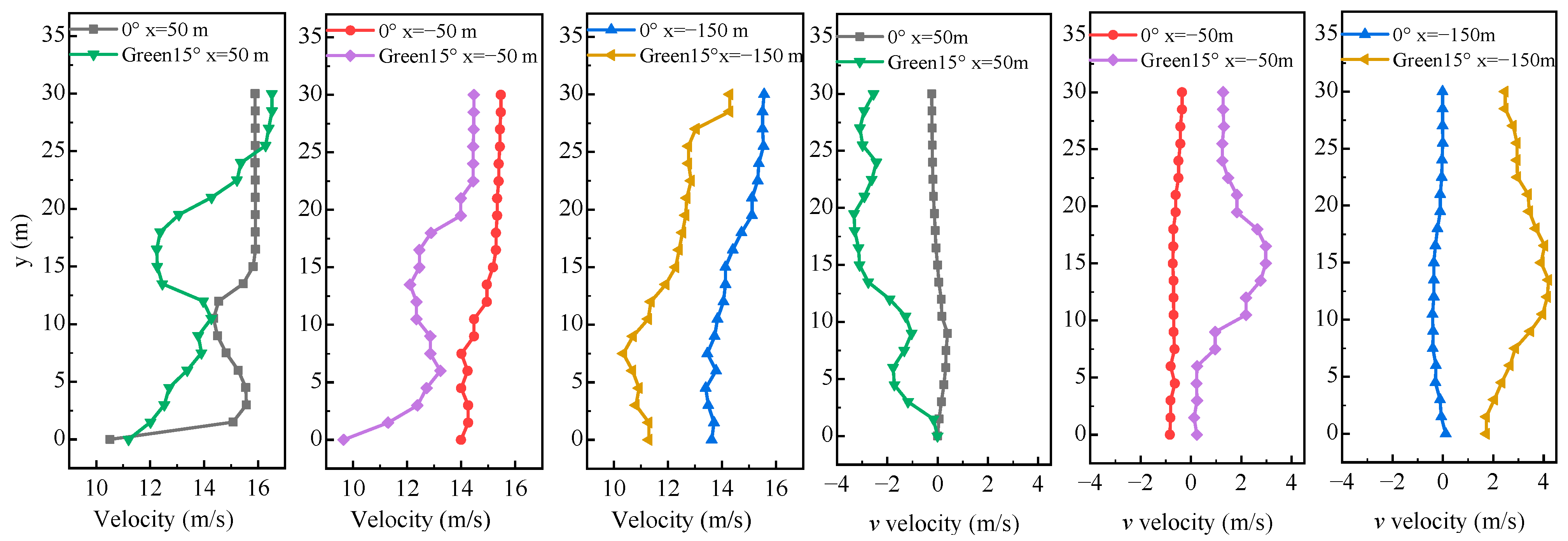
• A full-size simulation using the DDES method was carried out to predict the flow field of the aircraft carrier under stationary conditions. The airwake distribution showed an identical feature as that which appeared in the scaled-down model. The overall speed of the fall line decreased for the green 15° wind case while maintaining considerable fluctuations. The downwash area was reduced, but the upwash flow was more intense. When a carrier-based aircraft entered the transition zone between the upwash and downwash regions of the aircraft carrier’s wake, the lift of the aircraft decreased rapidly, posing a safety risk for landing.
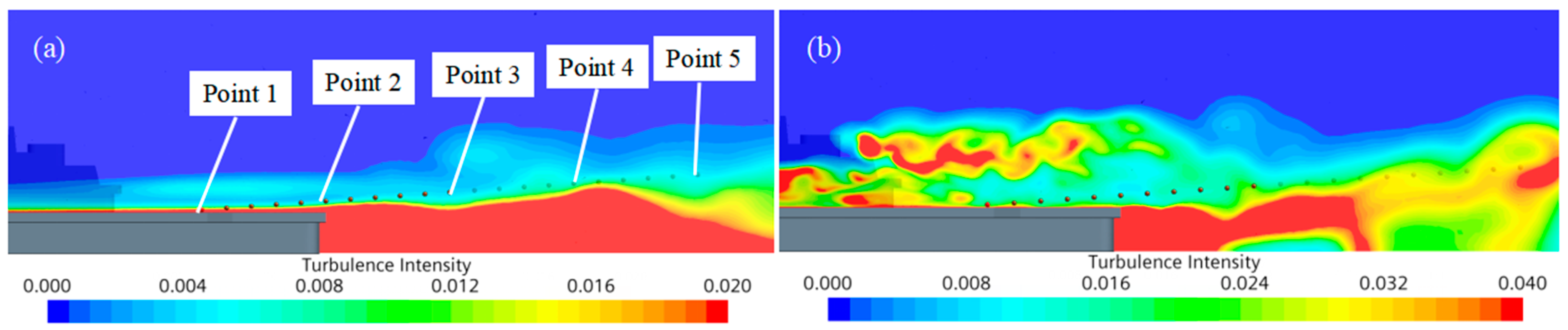
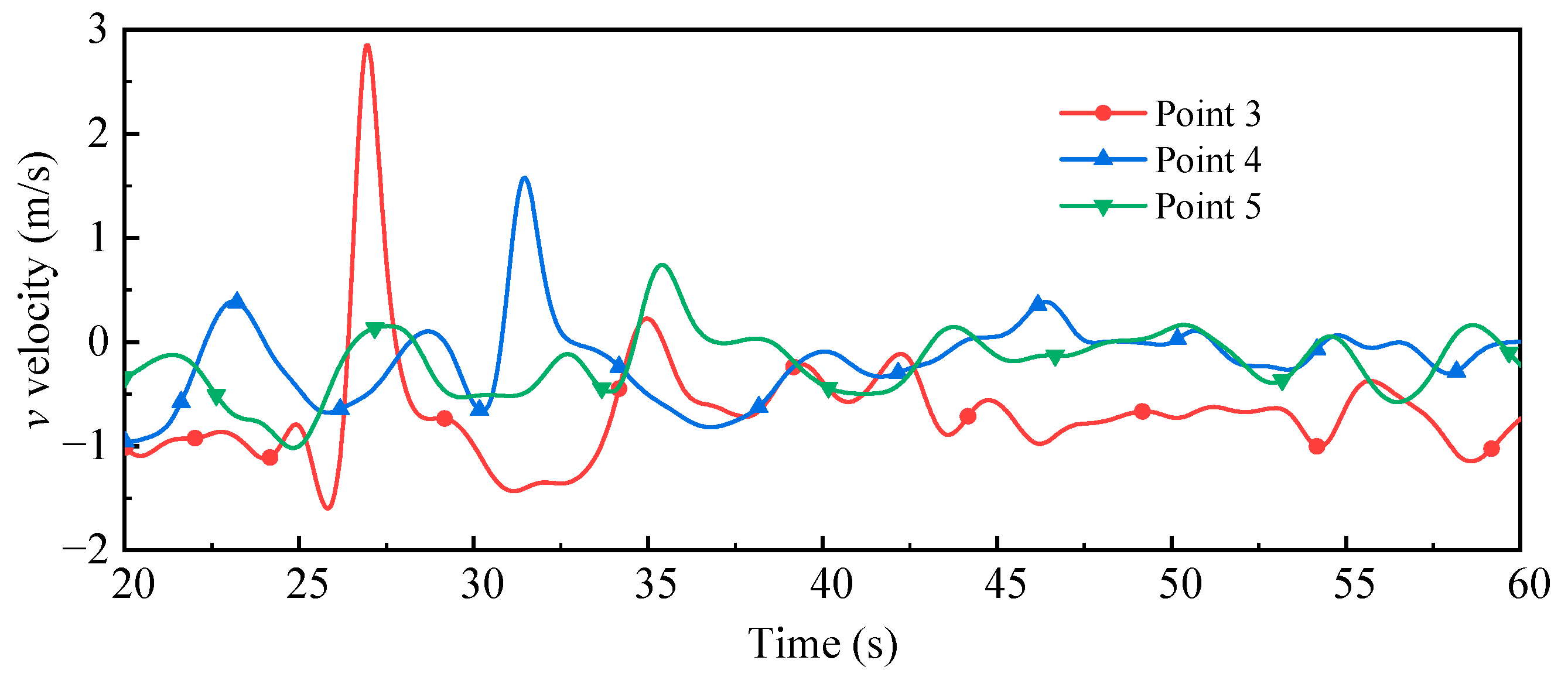
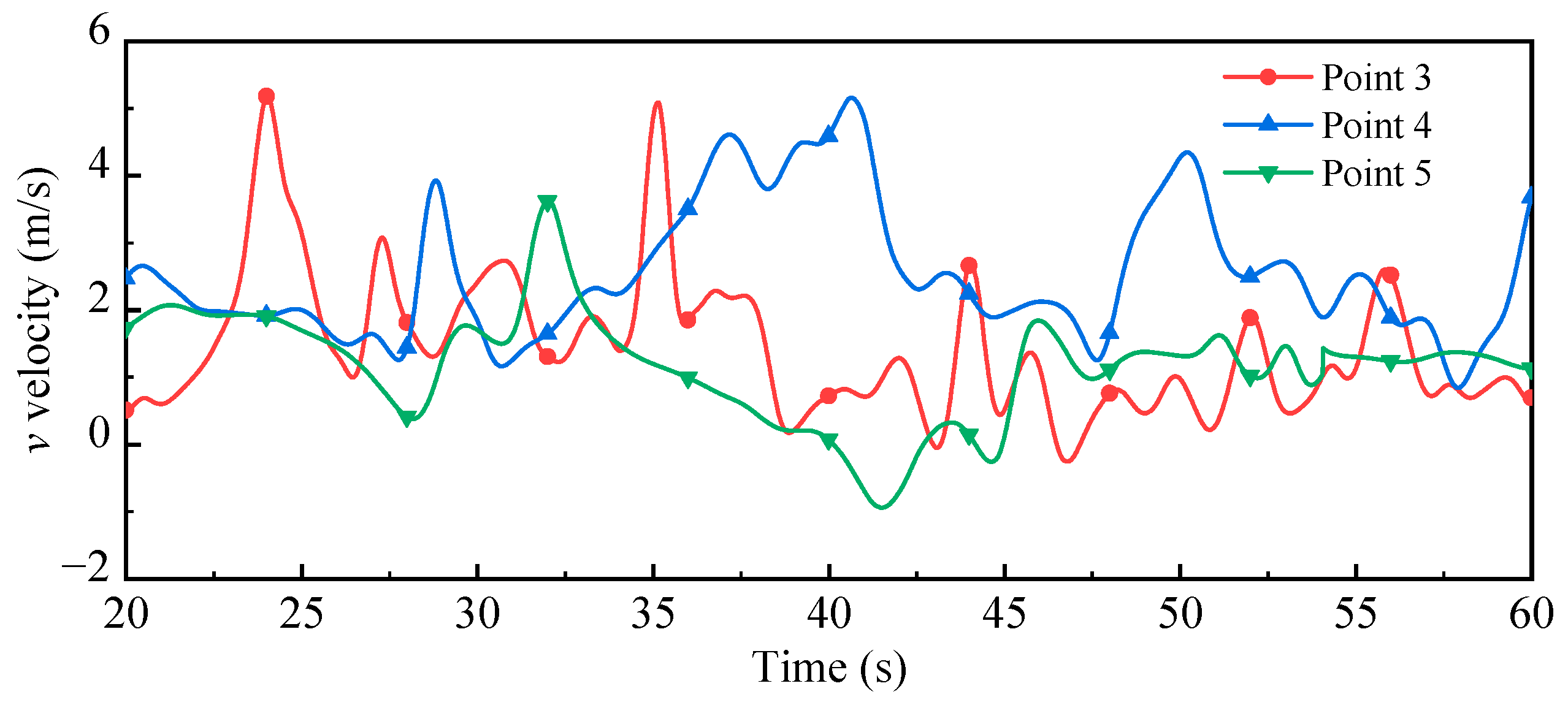
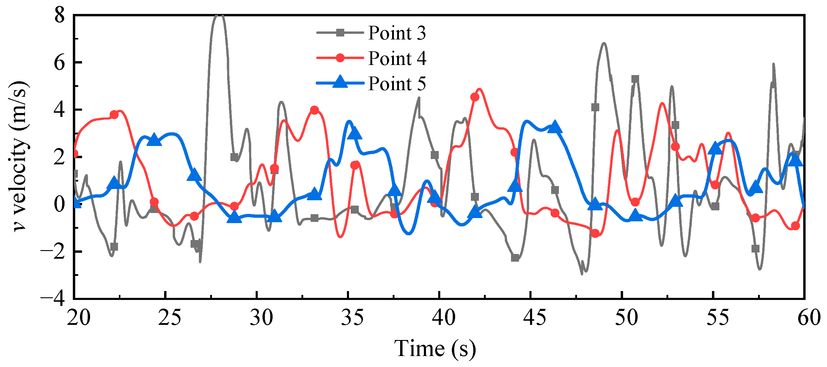
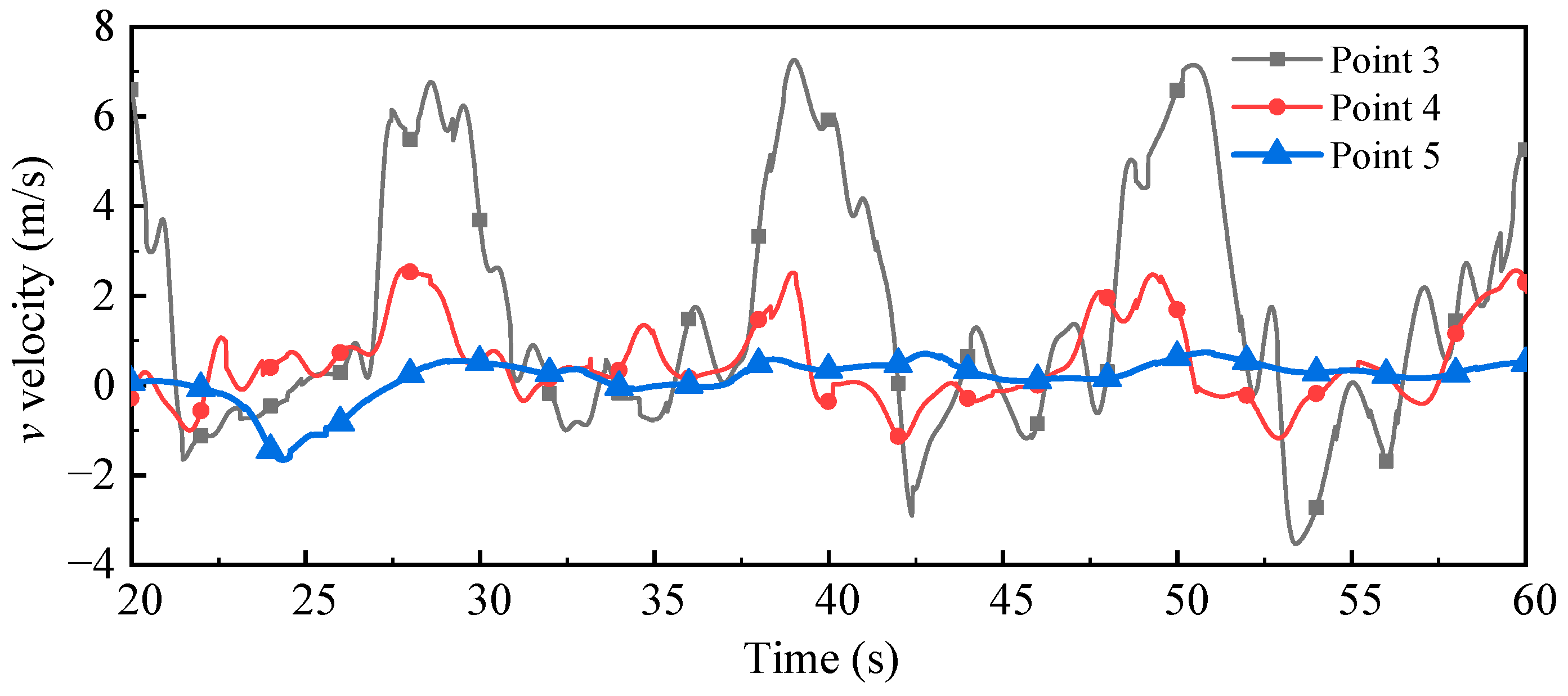
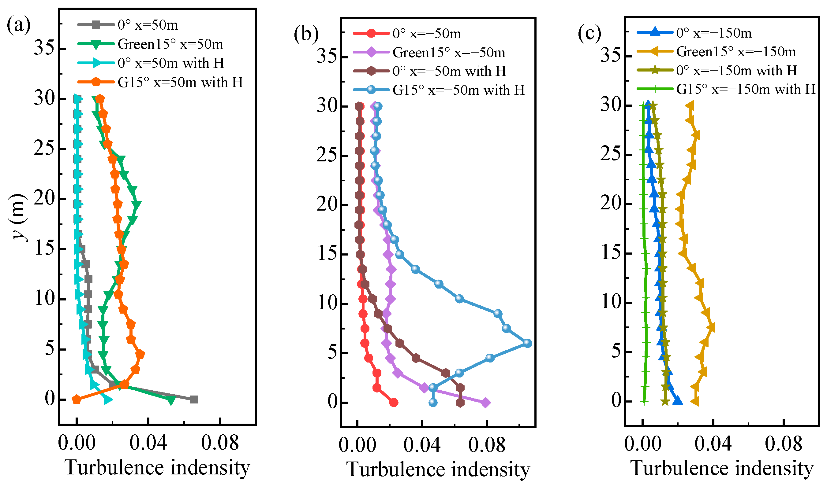
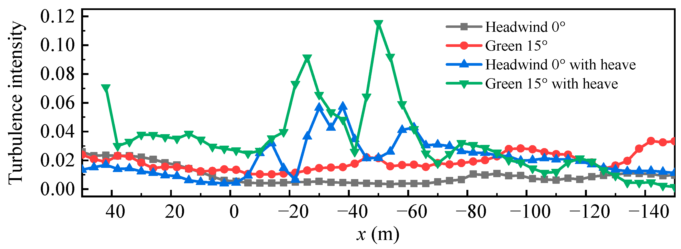
• The stern vortex distribution was investigated under swaying conditions. The airwake area was found to be increased with the swaying motion. The aft edge of the stern deck showed a periodic separation vortex. This phenomenon has not been observed behind the deck of a stationary hull. The periodicity and amplitude of the near-landing point intensified under the green 15° wind with heave. The effect of airwake diminished after 150 m. Compared to a stationary hull, heave motion under headwind conditions increased the vertical velocity component range at Point 3 by 144%, and by 66.7% under green 15° wind. With the hull heave conditions, the turbulence intensity along the approach line of the aircraft increased significantly, which was the critical area for the aircraft landing. The heave motion of the aircraft carrier increased the fluctuation of the wake, leading to greater fluctuations in aircraft lift, which was unfavorable for the control of the flight system and the pilot.
• It was found that the vertical velocity component contained more energy in the ship swaying state according to PSD analysis. Further, the signals at about 0.1–1 Hz over the approach line consisted of the most energy, which was induced by ship sway.

References

- Forrest, J.S.; Kaaria, C.H.; Owen, I. Evaluating ship superstructure aerodynamics for maritime helicopter operations through CFD and flight simulation. Aeronaut. J. 2016, 120, 1578–1603. [Google Scholar] [CrossRef]
- Owen, I.; White, M.D.; Padfield, G.D.; Hodge, S.J. A virtual engineering approach to the ship-helicopter dynamic interface; a decade of modelling and simulation research at the university of liverpool. Aeronaut. J. 2017, 121, 1833–1857. [Google Scholar] [CrossRef]
- Reddy, K.R.; Toffoletto, R.; Jones, K. Numerical Simulation of Ship Airwake. Comput. Fluids 2000, 29, 451–465. [Google Scholar] [CrossRef]
- Zan, S.J. Surface Flow Topology for a Simple Frigate Shape. Can. Aeronaut. Space J. 2001, 47, 33–43. [Google Scholar]
- Mora, R.B. Flow field velocity on the flight deck of a frigate. Proc. Inst. Mech. Eng. Part G J. Aerosp. Eng. 2014, 228, 2674–2680. [Google Scholar] [CrossRef]
- Polsky, S.; Naylor, S. CVN Airwake Modeling and Integration: Initial Steps in the Creation and Implementation of a Virtual Burble for F-18 Carrier Landing Simulations. Synthese 2015, 66, 405–435. [Google Scholar]
- Shipman, J.; Arunajatesan, S.; Peter Cavallo, P.; Sinha, N.; Polsky, S. Dynamic CFD Simulation of Aircraft Recovery to an Aircraft Carrier. In Proceedings of the 26th AIAA Applied Aerodynamics Conference, Honolulu, HI, USA, 18–21 August 2008. [Google Scholar] [CrossRef]
- Kelly, M.F.; White, M.; Owen, I. Using airwake simulation to inform flight trials for the Queen Elizabeth Class Carrier. In Proceedings of the INEC 2016, 13th International Naval Engineering Conference, Bristol, UK, 26–28 April 2016. [Google Scholar]
- Polsky, S. CFD Prediction of Airwake Flowfields for Ships Experiencing Beam Winds. In Proceedings of the 21st AIAA Applied Aerodynamics Conference, Orlando, FL, USA, 23–26 June 2003. [Google Scholar] [CrossRef]
- Zhang, J.; Minelli, G.; Rao, A.N.; Basara, B.; Bensow, R.; Krajnović, S. Comparison of PANS and LES of the flow past a generic ship. Ocean Eng. 2018, 165, 221–236. [Google Scholar] [CrossRef]
- Rahimpour, M.; Oshkai, P. Experimental investigation of airflow over the helicopter platform of a polar icebreaker. Ocean Eng. 2016, 121, 98–111. [Google Scholar] [CrossRef]
- Rosenfeld, N.; Kimmel, K.; Sydney, A.J. Investigation of Ship Topside Modeling Practices for Wind Tunnel Experiments. In Proceedings of the Aiaa Aerospace Sciences Meeting, Kissimmee, FL, USA, 5–9 January 2015. [Google Scholar] [CrossRef]
- Shukla, S.; Singh, S.N.; Sinha, S.S.; Vijayakumar, R. Comparative assessment of URANS, SAS and DES turbulence modeling in the predictions of massively separated ship airwake characteristics. Ocean. Eng. 2021, 229, 108954. [Google Scholar] [CrossRef]
- Shukla, S.; Sinha, S.S.; Singh, S.N. Ship-helo coupled airwake aerodynamics: A comprehensive review. Prog. Aerosp. Sci. 2019, 106, 71–107. [Google Scholar] [CrossRef]
- Spalart, P.R. Comments on the feasibility of LES for wings, and on a hybrid RANS/LES approach. In Proceedings of the First AFOSR International Conference on DNS/LES, Ruston, LA, USA, 4–8 August 1997. [Google Scholar]
- Spalart, P.R.; Deck, S.; Shur, M.L.; Squires, K.D.; Strelets, M.K.; Travin, A. A New Version of Detached-eddy Simulation, Resistant to Ambiguous Grid Densities. Theor. Comput. Fluid Dyn. 2006, 20, 181–195. [Google Scholar] [CrossRef]
- Spalart, P.R.; Squires, K.D. The Status of Detached-Eddy Simulation for Bluff Bodies; Springer: Berlin/Heidelberg, Germany, 2004. [Google Scholar]
- Strelets, M. Detached eddy simulation of massively separated flows. In Proceedings of the 39th Aerospace Sciences Meeting and Exhibit, Reno, NV, USA, 8–11 January 2001. [Google Scholar] [CrossRef]
- Forrest, J.S.; Owen, I. An investigation of ship airwakes using Detached-Eddy Simulation. Comput. Fluids 2010, 39, 656–673. [Google Scholar] [CrossRef]
- Watson, N.A.; Kelly, M.F.; Owen, I.; Hodge, S.J.; White, M.D. Computational and experimental modelling study of the unsteady airflow over the aircraft carrier HMS Queen Elizabeth. Ocean Eng. 2019, 172, 562–574. [Google Scholar] [CrossRef]
- Owen, I.; Lee, R.; Wall, A.; Fernandez, N. The NATO generic destroyer-a shared geometry for collaborative research into modelling and simulation of shipboard helicopter launch and recovery. Ocean. Eng. 2021, 228, 108428. [Google Scholar] [CrossRef]
- Nisham, A.; Terziev, M.; Tezdogan, T.; Beard, T.; Incecik, A. Prediction of the aerodynamic behaviour of a full-scale naval ship in head waves using Detached Eddy Simulation. Ocean. Eng. 2021, 222, 108583. [Google Scholar] [CrossRef]
- Cadot, O. Experimental and numerical analysis of the bi-stable turbulent wake of a rectangular flat-backed bluff body. Phys. Fluids 2020, 32, 105111. [Google Scholar] [CrossRef]
- Kanninen, P.; Peltonen, P.; Vuorinen, V. Full-scale ship stern wave with the modelled and resolved turbulence including the hull roughness effect. Ocean. Eng. 2022, 245, 110434. [Google Scholar] [CrossRef]
- Boudreau, M.; Dumas, G.; Veilleux, J.C. Assessing the Ability of the DDES Turbulence Modeling Approach to Simulate the Wake of a Bluff Body. Aerospace 2017, 4, 41. [Google Scholar] [CrossRef]
- Yuan, W.; Wall, A.; Lee, R. Combined numerical and experimental simulations of unsteady ship airwakes. Comput. Fluids 2018, 172, 29–53. [Google Scholar] [CrossRef]
- Menter, F.R. Zonal Two Equation k-w Turbulence Models For Aerodynamic Flows. In Proceedings of the 23rd fluid Dynamics, Plasmadynamics, and Lasers Conference, Orlando, FL, USA, 6–9 July 1993; Volume 93. NASA STI/Recon Technical Report N. [Google Scholar] [CrossRef]
- Gritskevich, M.S.; Garbaruk, A.V.; Schütze, J.; Menter, F.R. Development of DDES and IDDES Formulations for the k-ω Shear Stress Transport Model. Flow Turbul. Combust. 2012, 88, 431–449. [Google Scholar] [CrossRef]
- Chesshire, G.; Henshaw, W.D. A Scheme for Conservative Interpolation on Overlapping Grids. SIAM J. Sci. Comput. 1994, 15, 819–845. [Google Scholar] [CrossRef]
- Hadzic, H. Development and Application of Finite Volume Method for the Computation of Flows around Moving Bodies on Unstructured, Overlapping Grids. Ph.D. Thesis, Technische Universität Harburg, Hamburg, Germany, 2006. [Google Scholar]
- Hunt, J.; Wray, A.A.; Moin, P. Eddies, streams, and convergence zones in turbulent flows. In Proceedings of the Studying Turbulence Using Numerical Simulation Databases, 2, 27 June–22 July 1988; pp. 193–208. Available online: https://ntrs.nasa.gov/citations/19890015184 (accessed on 2 August 2024).
- Zhang, J.; Minelli, G.; Basara, B.; Bensow, R.; Krajnović, S. Yaw effect on bi-stable air-wakes of a generic ship using large eddy simulation. Ocean. Eng. 2020, 219, 108164. [Google Scholar] [CrossRef]
- Greenwell, D.I.; Barrett, R.V. Inclined screens for control of ship air wakes. In Proceedings of the AIAA paper 2006-3502, 3rd AIAA Flow Control Conference, San Francisco, CA, USA, 5–8 June 2006. [Google Scholar]
- Healey, J.V. Establishing a database for flight in the wakes of structures. J. Aircraft. 1992, 29, 559–564. [Google Scholar] [CrossRef]
- Garratt, J.R. Review: The atmospheric boundary layer. Earth-Sci. Rev. 1994, 37, 89–134. [Google Scholar] [CrossRef]
Disclaimer/Publisher’s Note: The statements, opinions and data contained in all publications are solely those of the individual author(s) and contributor(s) and not of MDPI and/or the editor(s). MDPI and/or the editor(s) disclaim responsibility for any injury to people or property resulting from any ideas, methods, instructions or products referred to in the content. |
© 2024 by the authors. Licensee MDPI, Basel, Switzerland. This article is an open access article distributed under the terms and conditions of the Creative Commons Attribution (CC BY) license (https://creativecommons.org/licenses/by/4.0/).
Share and Cite
Yang, X.; Li, B.; Ren, Z.; Tian, F. Numerical Simulation of the Unsteady Airwake of the Liaoning Carrier Based on the DDES Model Coupled with Overset Grid. J. Mar. Sci. Eng. 2024, 12, 1598. https://doi.org/10.3390/jmse12091598
Yang X, Li B, Ren Z, Tian F. Numerical Simulation of the Unsteady Airwake of the Liaoning Carrier Based on the DDES Model Coupled with Overset Grid. Journal of Marine Science and Engineering. 2024; 12(9):1598. https://doi.org/10.3390/jmse12091598
Chicago/Turabian StyleYang, Xiaoxi, Baokuan Li, Zhibo Ren, and Fangchao Tian. 2024. "Numerical Simulation of the Unsteady Airwake of the Liaoning Carrier Based on the DDES Model Coupled with Overset Grid" Journal of Marine Science and Engineering 12, no. 9: 1598. https://doi.org/10.3390/jmse12091598