Exploring Water Level Sensitivity for Metropolitan New York during Sandy (2012) Using Ensemble Storm Surge Simulations

Abstract

This paper describes storm surge simulations made for Sandy (2012) for the Metropolitan New York (NYC) area using the Advanced Circulation (ADCIRC) model forced by the Weather Research and Forecasting (WRF) model. The atmospheric forecast uncertainty was quantified using 11-members from an atmospheric Ensemble Kalman Filter (EnKF) system. A control WRF member re-initialized every 24 h demonstrated the capability of the WRF-ADCIRC models to realistically simulate the 2.83 m surge and 4.40 m storm tide (surge + astronomical tide) above mean lower low water (MLLW) for NYC. Starting about four days before landfall, an ensemble of model runs based on the 11 “best” meteorological predictions illustrate how modest changes in the track (20–100 km) and winds (3–5 m s⁻¹) of Sandy approaching the New Jersey coast and NYC can lead to relatively large (0.50–1.50 m) storm surge variations. The ensemble also illustrates the extreme importance of the timing of landfall relative to local high tide. The observed coastal flooding was not the worst case for this particular event. Had Sandy made landfall at differing times, locations and stages of the tide, peak water levels could have been up to 0.5 m higher than experienced.

1. Introduction

1.1. Background

Hurricane Sandy, which struck Metropolitan New York (NYC), New Jersey (NJ), and Long Island (LI) on 29 October 2012, resulted in 72 deaths and over $50 billion dollars (US$ 2012) in property damage [1]. Sandy began as a disturbance off the African coast on 11 October 2012 [1], and developed into a major hurricane at 06:00 UTC, 25 October, just south of Cuba.

An upper-level trough moving eastward along the US-Canadian border helped steer Sandy northward, while a blocking ridge downstream over the northern Atlantic ultimately forced Sandy westward towards the New Jersey coast [2]. After some weakening over Cuba due to topography, Sandy fell below hurricane strength. As Sandy moved northward along the U.S. east coast, the interaction of the upper-level trough and the warm Gulf Stream sea surface temperatures (SSTs) resulted in a re-intensification to a category 1. Additionally, the radial extent of tropical storm force winds around Sandy increased to 2300 km at 12:00 UTC, 28 October, as cold air wrapped around the vortex and formed a warm secluded frontal structure [2].

The National Weather Service (NWS) declassified Sandy as a hurricane just before landfall (21:00 UTC, 29 October) [3], but its unprecedented large size, slow progression, and track resulted in record-high storm surges along coastal New York and New Jersey [1]. The storm tide (surge + tide) for Sandy was around 4.40 m above mean lower low water (1.0 m; MLLW; 1983–2001) at the southern tip of Manhattan Island, which was the largest storm-tide in recorded history (150 year) at this location.

The sustained winds (36 m s⁻¹) were category 1 hurricane-equivalent (minimum pressure 945 hPa) when Sandy made landfall over southern New Jersey [1]. Tropical storm force winds extended over 500 km to the north and east of the system (see NHC Best Track 2014 Figure 1), and the significant wave height peaked at around 10 m at National Data buoy 44025 60 km south of Long Island [4]. The official National Hurricane Center (NHC) track errors for Hurricane Sandy were about 50.0% lower than the long-term mean track error for 48-h to 96-h track forecasts, which demonstrates that Sandy’s operational forecast was relatively accurate [1].

Experimental real-time forecasts during Sandy, including the Pennsylvania State University (PSU) Weather Research and Forecasting (WRF)—Ensemble Kalman Filter (EnKF) system that assimilated airborne Doppler radar observations [5,6] were analyzed. At a forecast lead-time four to five days prior to landfall, nearly 18.0% of the PSU WRF-EnKF ensemble members did not predict United States landfall. Munsell and Zhang [6] showed that the uncertainty in the initial environmental steering-level flow over the tropics and Sandy’s subsequent interaction with the approaching mid-level trough resulted in much of the spread of the Sandy track forecasts.

Figure 1. Track of hurricane Sandy for the best track (bold cyan), control WRF member (bold black), and 11 ensemble WRF members (see legend) starting at 00:00 UTC, 26 October 2012 (symbols plotted every 12 h). The location of The Battery tide gauge for the verification is shown at the NYC location (blue cross).

Figure 1. Track of hurricane Sandy for the best track (bold cyan), control WRF member (bold black), and 11 ensemble WRF members (see legend) starting at 00:00 UTC, 26 October 2012 (symbols plotted every 12 h). The location of The Battery tide gauge for the verification is shown at the NYC location (blue cross).

Even for those tracks that predicted landfall within about 150 km of observed, the operational surge models in the region, including the NOAA extra tropical surge model [7,8], Stevens Institute NYHOPS (SIT-NYHOPS, Hoboken, NJ, USA; [9], and the Stony Brook Surge Model [10,11], under-predicted the surge by 0.50 to 1.0 m starting at a lead time of 48 h (not shown).

The SIT-NYHOPS under-prediction was at least partially the result of inferior wind forecasts from the operational models [12]. Forbes et al. [13] showed that the NWS Sea, Lake, and Overland Surges from Hurricanes (SLOSH) model [14] could realistically simulate the Sandy water levels using an ensemble of tracks and intensities from the National Hurricane Center. Both Forbes et al. [13] and Georgas et al. [12] illustrated that Sandy’s observed flooding was not a worst-case scenario for this event given the variations in Sandy’s track and phase of the tide landfall that might have occurred.

1.2. Motivation

Sandy’s atmospheric predictability has been extensively discussed in [6], but little information exists on how small changes in the track and intensity of Sandy might have changed regional storm surges. Forbes et al. (2014) [13] showed a large ensemble spread of surge predictions using SLOSH for Sandy around NYC, but did not discuss the origin of that water level spread. Wind and pressure forcing for SLOSH are geometrically circular, thus unrepresentative of the large asymmetries observed during Sandy. Georgas et al. (2014) [12] illustrated the tidal uncertainty aspect of Sandy’s water level prediction, but did not run SIT-NYHOPS days before landfall with an ensemble of forecasts.

Our study’s goal is not to fully quantify the storm surge probabilities of Sandy since only a subset of WRF forecasts from the PSU EnKF system were available for analysis. Rather, using a more limited ensemble of ~11 members, this paper addresses:

• How well can a storm surge ocean model predict Sandy’s surge if the track, winds and sea level pressure (SLP) from Sandy are reasonably well predicted?
• How does a shift in the track, timing (vis-à-vis tides), and wind intensity for Sandy translate into predicted storm-tide changes for the New York coastline?
• Given the ensemble envelope of storm surge predictions/timing uncertainties, how much worse might the flooding have been?

2. Data and Methods

Munsell and Zhang [6] presented the details of the WRF-EnKF Sandy runs, extending the analysis of Weng and Zhang [5] and Zhang et al. [15]. The EnKF system used an ensemble of WRF forecasts to estimate flow-dependent background error covariance for the data assimilation cycling. It assimilated NOAA hurricane hunter aircraft Doppler velocity observations to create a 60-member ensemble starting at 00:00 UTC, 26 October 2012, using the same model physics of Munsell and Zhang [6]. Three domains were used (27-, 9-, and 3-km resolution), with the inner two nested domains centered around and following the storm (dimensions of 2700 × 2700 km and 900 × 900 km, respectively, with 44 vertical levels and a model top at 10 hPa).

NOAA’s operational global forecast system (GFS) [16] was used for initial and boundary conditions, with the WRF ensemble initialized 6 to 12-h before the Doppler observations were ingested. EnKF analyses were used every 12-h to generate successive WRF forecasts. The WRF runs every 24-h (starting at 00:00 UTC, 25 October 2012) were used to construct a “control” member, in which the first 24-h from each run was used to force the ADCIRC [17].

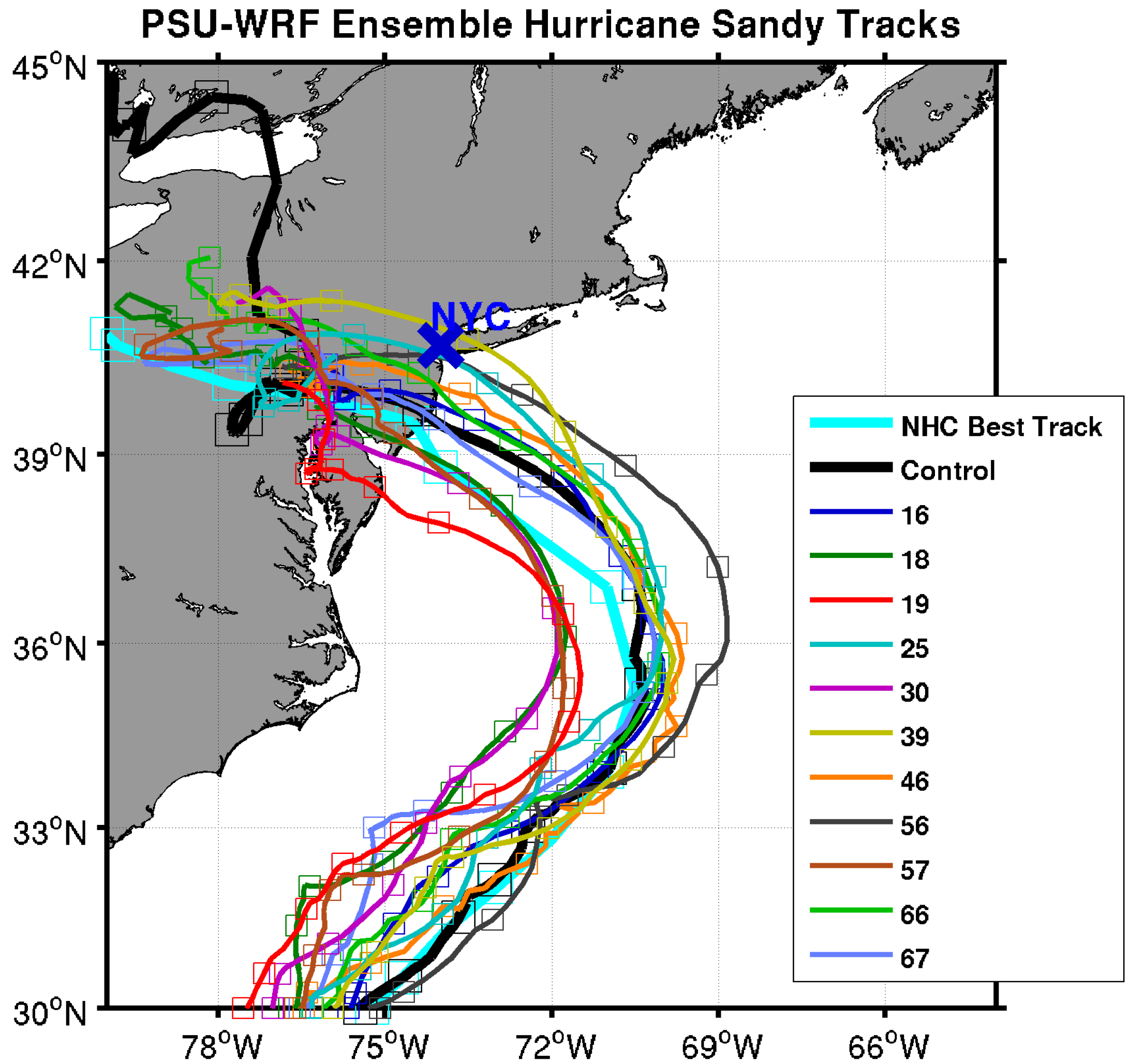
From the 60-member ensemble starting at 00:00 UTC, 26 October, a set of 11 members was chosen that were subjectively judged as the “best” performing members. Here “best” means that the track made landfall anywhere from coastal NY southward to the southern Maryland coastline (Figure 1). We chose these relatively accurate members to quantify how relatively small changes in the track can change NYC surge predictions, but not to determine the overall probability of the event with a 4-day lead-time.

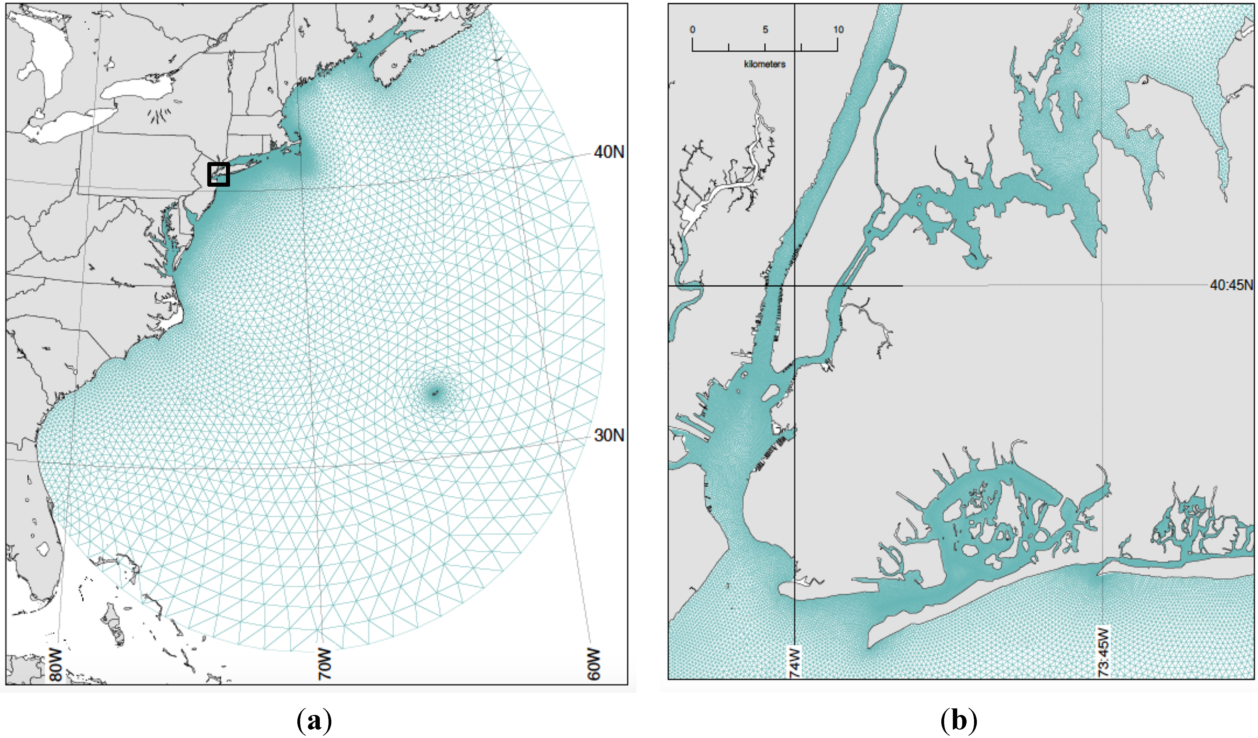
The grid for ADCIRC extends from the eastern seaboard from Central Florida to Nova Scotia, Canada and eastward into the central North Atlantic Ocean in a semi-circular arc (Figure 2; 184,534 node points). This grid greatly improved near-shore coastal bathymetric resolution to the grid used previously by DiLiberto et al. [11] and extended much further along the eastern seaboard in both directions. A decision was made not to extend the grid further as then the ocean model’s grid would have been considerably larger that the overlying WRF grid and various tests on smaller grids showed that the final range chosen was sufficient.

Figure 2. (a) Domain of the ADCIRC model, extending from mid State of Florida (FL) to the Atlantic coast of Nova Scotia, Canada (NS), indicated by the black nodes. (b) Zoom in for the small black box in (a) for the region around NYC and western Long Island. The sizes of elements range from ~7 m in inner bays and estuaries to ~70 km along the outer ocean boundary. The grid has 184,534 nodes.

Figure 2. (a) Domain of the ADCIRC model, extending from mid State of Florida (FL) to the Atlantic coast of Nova Scotia, Canada (NS), indicated by the black nodes. (b) Zoom in for the small black box in (a) for the region around NYC and western Long Island. The sizes of elements range from ~7 m in inner bays and estuaries to ~70 km along the outer ocean boundary. The grid has 184,534 nodes.

ADCIRC is usually run in a 2-D vertically integrated mode for fastest operation for surge prediction studies [18,19]. It also has a 3-D mode, which allows for vertical shear in the horizontal tidal and wind-driven currents. (Note that this is not a baroclinic mode per se since water density is not specified and the layers are spaced equidistant between the surface and the bottom at each node). The operational version for the NYC region, described by Colle et al. [20] and DiLiberto et al. [11], is normally run in a 2-D (barotropic) configuration with no wave coupling [10]. However, for this analysis of Sandy storm surges, ADCIRC was run with 1, 3, 5, and 7-vertical layer configuration coupled with the Simulating Waves Nearshore (SWAN) wave generation model [21]. Orton et al. [22] showed that stratification can be important for this region, since ignoring it can lead to some surge underprediction, but this process was not included in our ADCIRC runs. SWAN ingests WRF 10-m wind predictions to create radiation wave stresses, which act as additional terms in the momentum equations that characterize coastal setup due to breaking waves along and near the shoreline. SWAN allows for shoaling, refraction and diffraction (including frequency shifting due to currents). Both ADCIRC and SWAN were run on the same non-structured triangular mesh grid with 184,534 node points. The ADCIRC time step was 4 s, while SWAN model ran stably with a 5-min time step.

ADCIRC was spun up two days before 00:00 UTC, 26 October, using the M2, K1, O1, N2, S2, M4, M6, S4, and MS4 tidal constituents [23] along the open boundary (Figure 2). Starting at 0000 UTC 25 October, 10-m winds from an earlier WRF-EnKF control forecast were taken every 15 min from the 9- and 3-km WRF domains to derive ADCIRC wind stresses using the Garratt [24] drag formulation without a cap since there is considerable uncertainty in regard to what the actual cap should be (e.g., Weisberg et al [25]).

Between 00:00 UTC, 25 October, and 00:00 UTC, 26 October, the surface wind and pressures within ADCIRC were linearly increased during this final one-day spin up period. The 9-km WRF domain was used for the surface wind stresses and surface pressures for those portions of the ADCIRC domain lying outside the 3-km WRF domain. The observed storm-tide and storm surge levels at The Battery (NYC in Figure 1) were taken from NOAA [26].

3. Results

3.1. Control Run Surge Simulations

Figure 1 shows the National Hurricane Center (NHC) best track (bold cyan), the control member (bold black), and the 11 WRF ensemble members starting at 00:00 UTC, 26 October 2012. The control (CTL) run, which was restarted every 24 h, as described above, realistically predicted Sandy’s track (the modeled storm made landfall +/−24 h to the observed landfall time and +/−300 km to the observed landfall location). The CTL provides one of the more realistic simulations as compared to the other ensemble members given its 24-h restarts, which minimize the growth of initial condition error. Starting at 12:00 UTC, 29 October, Sandy’s track was directed northwestward towards the southern NJ coast.

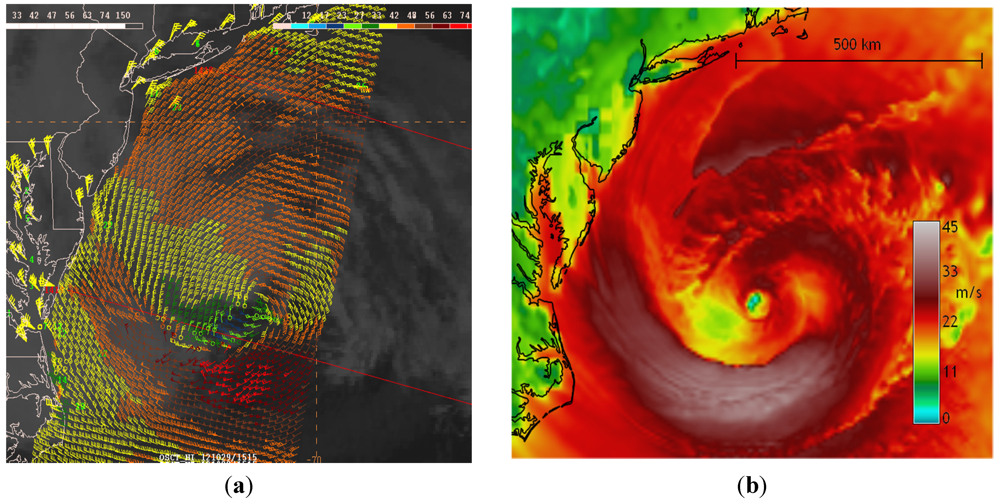
Figure 3. (a) Scatterometer surface winds (colored in kts and full barb = 10 kts) at 12:00 UTC, 29 October 2012; (b) Same as (a) except for the control WRF run (hour 12 forecast).

Figure 3. (a) Scatterometer surface winds (colored in kts and full barb = 10 kts) at 12:00 UTC, 29 October 2012; (b) Same as (a) except for the control WRF run (hour 12 forecast).

Figure 3 shows a 12-h forecast from the CTL run valid at 12:00 UTC, 29 October, as well as surface winds derived from Indian Space Research Organization’s (IRSO) Oceansat-2 scatterometer [27]. The areal extent of Sandy (with tropical storm force winds >18 m s⁻¹) extended >500 km NE from the center. The strongest winds were to the south of center within a developing bent-back front (Galarneau et al. [2]).

The Battery surge gradually increased from 0.30 to 1.0 m between 00:00 UTC, 28 October, to 12:00 UTC, 29 October (Figure 4a). The CTL underestimated this gradual increase in surge on the 28 October by 0.20–0.30 m, which was a consequence of previous WRF forecasted inaccuracies. The observed peak surge of 2.83 m occurred at 02:00 UTC, 30 October, whereas the simulated peak surge also occurred around that time at ~3.0 m, but with some members predicting a peak surge about 12-h too soon.

Figure 4. (a) Storm surge (in meters) at The Battery, NYC for the observed (bold red), control WRF-ADCIRC member (bold black), and 11 ensemble WRF-ADCIRC members (see legend) from 00:00 UTC, 28 October 2012, to 00:00 UTC, 31 October; (b) Same as (a) except for the total water level (surge + tide) in meters above mean lower low water (MLLW; 1.0 m; 1983–2001).

Figure 4. (a) Storm surge (in meters) at The Battery, NYC for the observed (bold red), control WRF-ADCIRC member (bold black), and 11 ensemble WRF-ADCIRC members (see legend) from 00:00 UTC, 28 October 2012, to 00:00 UTC, 31 October; (b) Same as (a) except for the total water level (surge + tide) in meters above mean lower low water (MLLW; 1.0 m; 1983–2001).

The peak storm tide (surge + astronomical tide) of around 4.30 m (MLLW) was predicted within 0.20 m by the CTL run (Figure 3b). Sandy’s peak surge occurred close to a local high tide and a bi-weekly spring tide. If Sandy had made landfall about 6 h earlier, around low tide, the storm tide would have been around 3.0 m (MLLW), flooding would have been much less severe and comparable to the December 1992 nor-easter [20].

The ADCIRC was verified at several other stations around the region (not shown). The storm tide was well simulated (within 10% of the observations) at Bergen Point near the Battery, as well as to the south along the southern New Jersey coast (e.g., Atlantic City), while the ADCIRC peak water levels were 0.5 to 1.0 m too low over western and eastern Long Island Sound stations. This underprediction was mainly the result of the CTL storm arriving 1–2 h too early when the tide was rapidly increasing. This 1–2 h timing error was less critical for the Battery, since it was around a high tide.

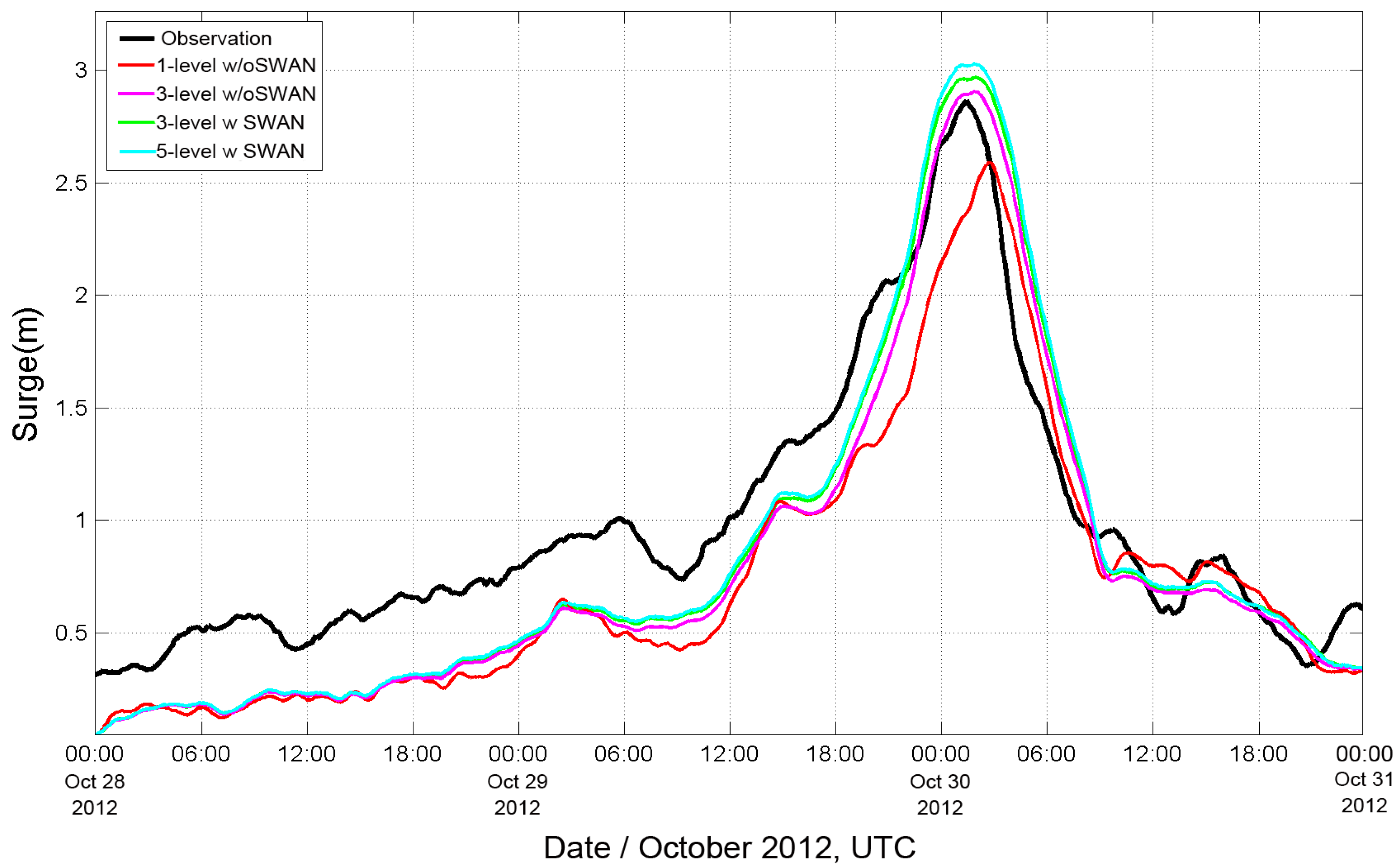
3.2. ADCIRC 2D and 3D Simulations

Water level simulations were sensitive to the number of ADCIRC vertical levels used. When ADCIRC was run in a barotropic 2-D (one vertical level) mode (e.g., DiLiberto et al. [11]), the surge was consistently under-forecasted by around 0.50 m and was delayed by a few hours (Figure 5). Weisberg and Zheng [28] showed that the 2D mode may overestimate the bottom stress and thus underestimate the surge.

Figure 5. Simulations of surge using different configurations of 2D and 3D ADCIRC (3 and 5-vertical layers) and with or without SWAN in predicting.

Figure 5. Simulations of surge using different configurations of 2D and 3D ADCIRC (3 and 5-vertical layers) and with or without SWAN in predicting.

3.3. Flooding Map for Sandy

Choosing three levels significantly improved the forecast but, when 5-layers were used, there was a modest change in the simulation of peak surge. Further, increasing the vertical resolution to seven levels did not significantly change the peak surge simulation (not shown). Additionally, the use of SWAN did not significantly alter the peak simulation of surge (not shown), which may be a consequence of the sheltered location of The Battery inside the upper bay of NY Harbor.

The ADCIRC surge forecast derived from the Sandy’s control run was used to create a first-order coastal flooding map of Sandy for Manhattan Island, western Brooklyn, and Queens along the East River (Figure 6). One challenge is that heights of seawalls surrounding the 870 km perimeter of New York Harbor are often not well documented. Rather than running ADCIRC in a wetting-drying mode, an estimate of local inundation using the control run was created by propagating sheets of water inland from the nearest ADCIRC coastal node (so-called “bathtubbing”) using a high horizontal resolution (~1 m) digital elevation map (DEM) of land elevation created using LIDAR data sets now available in the public domain [29,30]. This approach is justified when the source river water carries significantly more flow that the flooding sheets themselves; the effect of local flooding does not change the underlying river dynamics.

Figure 6. (a) 5-level ADCIRC w/SWAN-predicted Sandy inundation of central NYC and northern NJ during Sandy (colored blue), obtained with EnKF Control run, 2D ADCIRC, SWAN- and LIDAR- accurate topography; (b) Isometric projection of LIDAR-based 5-level ADCIRC w/SWAN-simulated flooding of the boroughs of Manhattan, Queens and Brooklyn (red and orange colors).

Figure 6. (a) 5-level ADCIRC w/SWAN-predicted Sandy inundation of central NYC and northern NJ during Sandy (colored blue), obtained with EnKF Control run, 2D ADCIRC, SWAN- and LIDAR- accurate topography; (b) Isometric projection of LIDAR-based 5-level ADCIRC w/SWAN-simulated flooding of the boroughs of Manhattan, Queens and Brooklyn (red and orange colors).

It is still a major challenge to create accurate street-by-street flooding maps since local flooding is very sensitive not only to elevation contours but also to local shifts in wind speed and direction at time and space scales atmospheric models cannot currently simulate. Additionally, street-level flooding cannot often be verified because of a lack of sensors and available operators during extreme weather events. Nevertheless, attempting to model inundation and disseminate this information at the street-by-street resolution remains an important challenge for emergency management and evacuation planning purposes and a topic of future scientific study.

3.4. Variations in Storm Tides around the Ensemble Forecast

The CTL simulations were compared with an 11-member ensemble started at 00:00 UTC, 26 October. There was a wide range of surge simulations derived from the ensemble (Figure 3a), ranging from 3.2–3.5 m in members 18, 66, 67 (nearly 0.1–0.4 m greater than observed and the CTL), to 1.5–2.0 m for 39 and 56. Member 46 generated the most accurate surge/storm tide forecast (Figure 3b), but its peak was delayed by 1–2 h. The timing of the surge with respect to the phase of the astronomical tide is critical to accurate peak storm-tide and surge simulations. Although members 66 and 67 had larger surges, they occurred close to local low tides, thus resulting in modest storm-tide levels.

To illustrate the importance of the timing of the arrival of the storm center on land, the predicted tidal phase was shifted in 30 min intervals from 13 h before landfall of CTL to 13 h after landfall and the tidal elevation added to the predicted surge at each time shift. This variation in the phase therefore represents all possible tidal phases over +/− one M₂ tidal period (T = 12.42-h). This addition of phase-shifted tides represents a convenient way of estimating the uncertainty in storm-tide (surge + tide) simulations using variations associated with each selected Sandy track (see Figure 1).

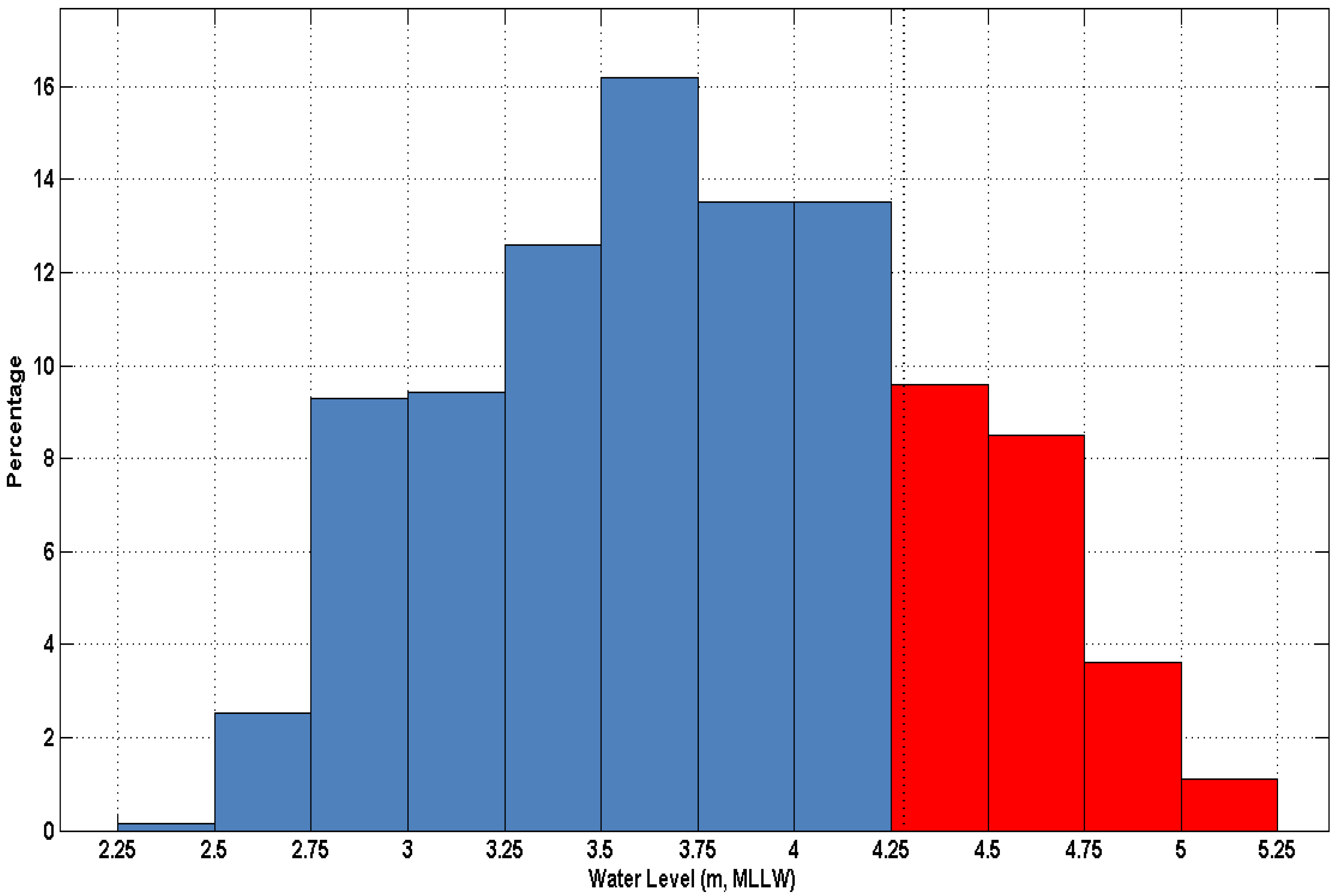
Thus, each of the 11 selected members produced 51 storm-tide simulations over two tidal cycles. These simulations were used to create a probability density function (PDF) of storm-tides (Figure 7). The PDF had a mean of 3.77 m (rel. to MLLW) and standard deviation of 0.59 m. Sandy’s peak water level in the CTL (~4.25 m) lies in the right tail of the PDF since it occurred near a local high tide, but around 20.0% of the storm-tide simulations (red-filled bins in Figure 7) are still greater than the CTL.

Figure 7. Probability distribution of peak water levels (storm tide rel. to MLLW) at The Battery created by shifting the phase of the tides in steps of 30 min between one tidal cycle before to one cycle following the time of landfall for each of the 11 wind ensemble field (see text for details).

Figure 7. Probability distribution of peak water levels (storm tide rel. to MLLW) at The Battery created by shifting the phase of the tides in steps of 30 min between one tidal cycle before to one cycle following the time of landfall for each of the 11 wind ensemble field (see text for details).

The right tail of the PDF represents surge simulations by members 66 and 67. Overall, Figure 7 illustrates that Sandy’s track did not lead to the worst possible coastal flooding for this particular event; the storm-tide could have been 0.50–0.75 m larger even using our small ensemble.

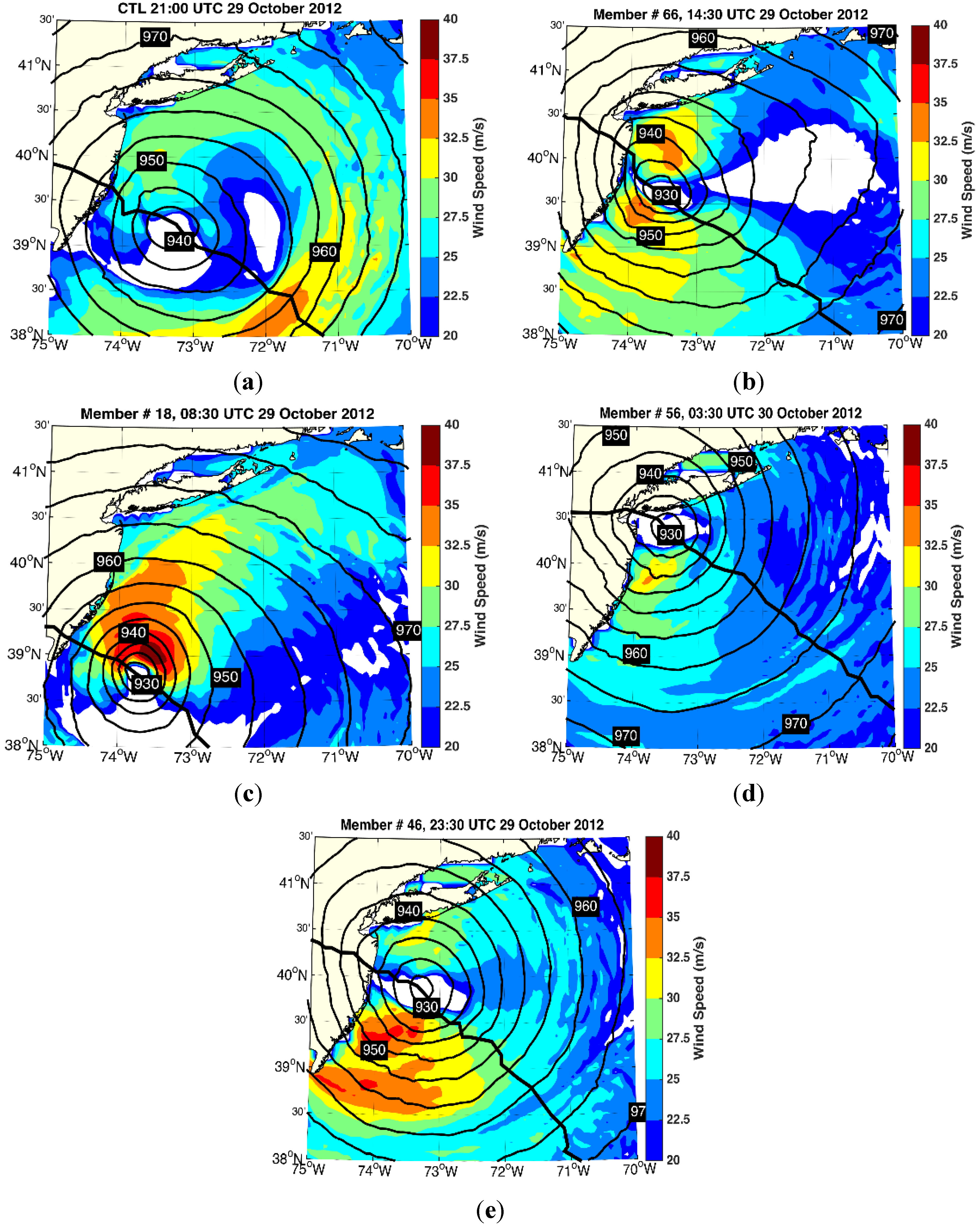
Figure 8. Mean sea-level pressure (every 10 hPa) and surface winds (color coded in m s⁻¹) for the (a) CTL; (b) 66; (c) 18; (d) 56; and (e) 46 members about an hour before landfall. The black line shows the track of the storm center.

Figure 8. Mean sea-level pressure (every 10 hPa) and surface winds (color coded in m s⁻¹) for the (a) CTL; (b) 66; (c) 18; (d) 56; and (e) 46 members about an hour before landfall. The black line shows the track of the storm center.

3.5. Wind and Sea Level Pressure Forecasts

In order to better explain the complexity of simulated surge and water levels, the distributions of 10-m winds and mean sea level pressure (MSLP) predicted locally at 30 min shortly before landfall were analysed for four-selected ensemble members (CTL, 66, 18, 56, 46), chosen because they led to the largest and lowest predicted surges at The Battery.

Ensemble member 66 winds were 3–5 m s⁻¹ stronger than the CTL north of the cyclone center (cf., Figure 8a,b) since member 66 central MSLP was around 10 hPa lower (more intense), and the member 66’s track was about 25 km further north. This resulted in about ~10.0% greater wind stress during the last few hours before landfall in member 66 than in the CTL south of Long Island (not shown).

Member 18 winds were stronger by 3–10 m s⁻¹ than the CTL north of the cyclone’s center (Figure 8c), but the track is 60 km to the south of the CTL. The winds in member 56 were similar to the CTL (Figure 8d), but its track took it right over NYC; therefore, the Battery was located away from the optimal surge generation region.

The winds north of the cyclone’s center for member 46 were only 1–2 m s⁻¹ greater than the CTL, and its track was located ~25 km farther to the north than the CTL, in a manner similar to member 66 (Figure 8e). Therefore, the surge for member 46 was relatively similar to the CTL’s. Our analysis shows that relatively modest variations in wind speed (around 3–5 m s⁻¹) and track variation (around 20–50 km), even with the inherent uncertainty in a four-day forecast, can produce significant changes (+/−0.5 m) to the storm-tide.

3.6. The Second Surge Originating from Long Island Sound

It is not generally understood that during superstorm Sandy, New York City was subjected to two interacting surges; the first propagated into the Upper Bay of New York Harbor through the main connection to the Atlantic Ocean, the Verrazano Narrows. The second surge originating in Long Island Sound (LIS), propagated along the NE-SW oriented axis of the Sound and then through the East River. In fact the surge in western LIS was the larger of the two surges, peaking at 3.86 m at 23:00 UTC, 29 October 2012, at the Kings Point NOAA tide station [31]. The highest storm tide experienced at Kings Point (western Long Island Sound) at 02:12 UTC, Oct 30 2012, was 4.36 m above MLLW. The two Sandy surges met in the general region of the lower East River where much flooding and resulting damage occurred.

However, because of the three-hour phase shift in the tidal phase across the ends of the East River tidal strait between the Battery and Kings Point [32] the storm tide in the western Sound was small as the peak surge occurred between low to mid-tide. This phase shift across the East River is a result of the fact that the tide propagating up the Hudson River is close to a progressive wave, while the tides in Long Island Sound are closer to a resonant standing wave [33,34]. The surge simulations presented in this paper take all these dynamical considerations into account since the ADCIRC model accurately includes the tides in Long Island and Block Island Sounds [35], as well as in New York Harbor at high resolution.

4. Conclusions

The Advanced Circulation (ADCIRC) ocean model forced using surface winds and mean sea-level pressure (MSLP) from a nested 3-km Weather Research and Forecasting (WRF) model following hurricane Sandy (2012) was used to explore variations in Sandy storm surge simulations at The Battery, located at the southern tip of Manhattan Island, New York City. The 10-m wind and MSLP forecast uncertainties were quantified using an 11-member Ensemble Kalman Filter (EnKF) system, initialized (at 00:00 UTC, 26 October 2012) four days before landfall. A control WRF member re-initialized every 24 h reproduced the observed storm surge at the Battery to within 10–20 cm, so the model is capable of producing an accurate forecast for this event if the atmospheric forcing is well predicted.

An 11-member storm surge ensemble starting approximately four days before landfall illustrated how relatively modest differences in the track (around 20–50 km) and intensity (around 3–5 m s⁻¹) of Sandy’s track, especially for a four-day forecast, can lead to relatively large storm surge variations of around 0.50 m. The ensemble approach also illustrates that the landfall timing relative to high tide is critical since Sandy’s surge, had it occurred during low tide (+/−6-h), would have resulted in significantly less flooding and damage.

The ensemble approach also illustrates that storm-tide levels observed during Sandy were likely not worst-case for this event since several members predicted surges at least 0.5 m greater. More specifically, about 20.0% of the scenarios using the ensemble approach produced storm-tides greater than observed. Overall, our study emphasizes the need for ensemble storm surge simulations for land-falling storm events.

Other tide stations in the area are being investigated and results will be published elsewhere.