Development of a Site-Specific Kinetic Model for Chlorine Decay and the Formation of Chlorination By-Products in Seawater

Abstract

Chlorine is used commonly to prevent biofouling in cooling water systems. The addition of chlorine poses environmental risks in natural systems due to its tendency to form chlorination by-products (CBPs) when exposed to naturally-occurring organic matter (NOM). Some of these CBPs can pose toxic risks to aquatic and benthic species in the receiving waters. It is, therefore, important to study the fate of residual chlorine and CBPs to fully understand the potential impacts of chlorination to the environment. The goal of this study was to develop improved predictions of how chlorine and CBP concentrations in seawater vary with time, chlorine dose and temperature. In the present study, chlorination of once-through cooling water at Ras Laffan Industrial City (RLIC), Qatar, was studied by collecting unchlorinated seawater from the RLIC cooling water system intake, treating it with chlorine and measuring time series of chlorine and CBP concentrations. Multiple-rate exponential curves were used to represent fast and slow chlorine decay and CBP formation, and site-specific chlorine kinetic relationships were developed. Through extensive analysis of laboratory measurements, it was found that only some of the control parameters identified in the literature were important for predicting residual chlorine and CBP concentrations for this specific location. The new kinetic relationships were able to significantly improve the predictability and validity of Generalized Environmental Modeling System for Surfacewaters (GEMSS)-chlorine kinetics module (CKM), a three-dimensional hydrodynamic and chlorine kinetics and transport model when applied for RLIC outfall studies using actual field measurements.

1. Introduction

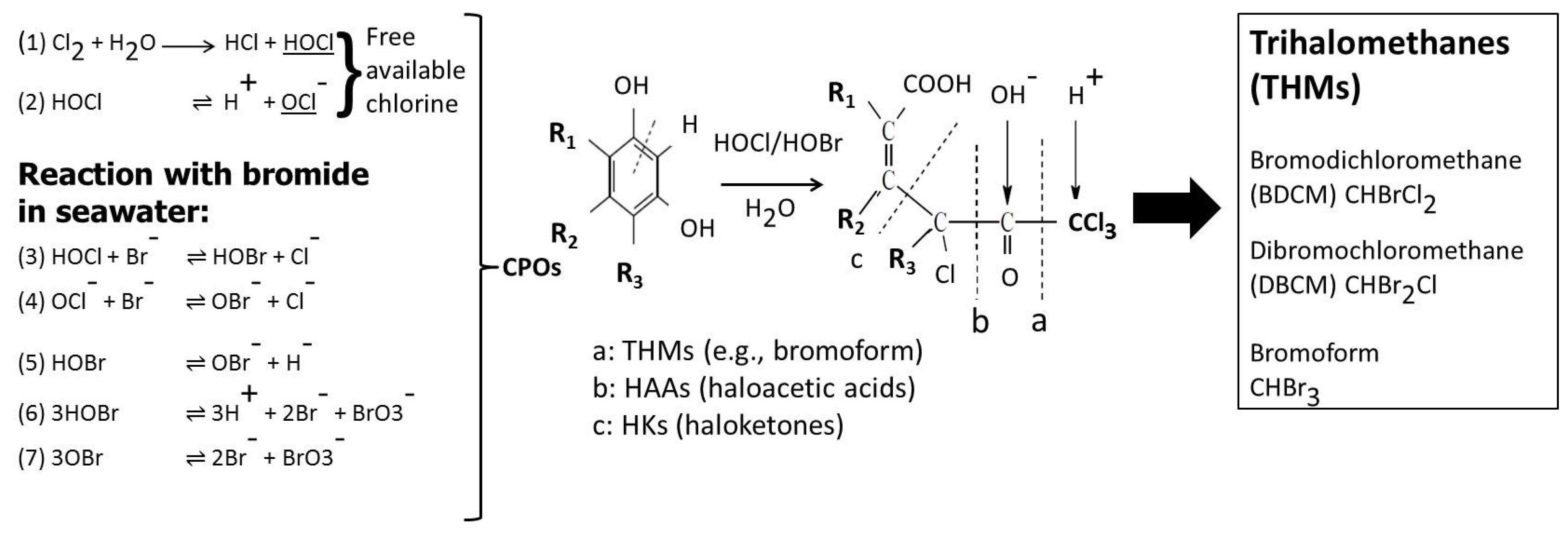
1.1. Chlorination

The liquefied natural gas (LNG) industry in Qatar located within Ras Laffan Industrial City (RLIC) utilizes more than 1 million m³/h of seawater for cooling demands. The total length of its seawater distribution network is approximately 6 km. Chlorine is extensively used as a powerful oxidizing agent for water treatments and for biofouling control. This is because it is a well-tested technology, has had a history of long-term worldwide industrial use and is of acceptable cost. Sodium hypochlorite (NaOCl, commonly termed chlorine) is the only biocide added to the RLIC seawater to prevent fouling and is produced on site by means of an electro-chlorination plant (ECP).

The chemistry of chlorine disinfection of seawater is complex [1,2,3]. In seawater, chlorine produces a mixture of hypochlorous acid (HOCl) and hypochlorite ion (OCl⁻). These rapidly react with the bromide ion to form a mixture of hypobromous acid (HOBr) and hypobromite ion (OBr⁻). The acute oxidants formed by chlorination are therefore short lived and are not persistent in seawater. A summary of the main chemical pathways is given in Figure 1. The environmental concern of chlorination is the production of numerous, and more persistent, compounds formed by complex reactions between chlorine/bromine and the organic constituents of seawater, collectively described as chlorination by-products (CBPs) [4,5,6]. Many CBPs are persistent and may be toxic to marine organisms subjected to long-term exposures [7,8]. Hence, new guidelines were established by the Qatari Ministry of Environment (MoE) for residual chlorine and CBPs in cooling discharge waters. The new regulations set by MoE specify that the maximum concentration of free residual chlorine is 0.05 mg/L at the discharge point. However, greater than 0.05 mg/L is permitted if a site-specific dispersion model is developed to demonstrate that the chlorine concentration does not exceed 0.01 mg/L at the edge of the mixing zone. To assist in the meeting of these new guidelines, a numerical hydrodynamic model was developed jointly by ExxonMobil Research Qatar (EMRQ) and Environmental Resource Management (ERM). The model was calibrated to predict the fate of residual chlorine and CBPs from industrial cooling water discharged from RLIC [9,10,11]. This model is novel, since the individual and cumulative effects of cooling water discharges from several outfalls are estimated in a single simulation instead of requiring separate model runs for each outfall.

Figure 1. Outline of the chlorine and bromide pathway modified from [12], with permission from © 1977 American Chemical Society. CPO stands for “chlorine-produced oxidant”.

Figure 1. Outline of the chlorine and bromide pathway modified from [12], with permission from © 1977 American Chemical Society. CPO stands for “chlorine-produced oxidant”.

Numerous empirical models for disinfectant decay and CBP formation have been proposed in recent decades for both fresh and seawater [13,14], but these models have, in most cases, not been generally applicable to all possible site conditions. The strength of any model lies in its flexibility and applicability, and a useful model should be able to accommodate site-specific factors, such as water quality (particularly variability in important variables, such as total and dissolved organic carbon and bromide) and operating conditions (e.g., pH, chlorine dose and temperature). The literature and our experience during the work described here suggest that an appropriate approach to this problem is to develop a standardized set of laboratory procedures to derive site-specific data on chlorine decay and CBP formation and to develop a robust, simplified site-specific mathematical model for predicting chlorine and CBP discharge concentrations.

1.2. Model Development

The modeling of chlorine decay is a complex task due to the difficulty related to ambient water quality. A large number of variables have been found to affect the fate of chlorine. As such, development of a universal model capable of predicting chlorine decay or CBP formation is virtually impossible without the aid of focused laboratory studies performed on the receiving water. Generic mathematical models for the decay of chlorine have been developed that can predict the formation of CBPs. These generic mathematical models form the basis of site-specific models, which take into account local ambient water quality and operating conditions.

A number of models have been developed to predict chlorine decay in cooling discharge systems [15,16,17]. The most popular model is the first-order decay model in which the chlorine concentration is assumed to decay exponentially.

$$C\left(t\right)= C_0{e}^{-kt}$$

(1)

where $\mathit{C}$ is the chlorine concentration at time $\mathit{t}$ and $\mathit{k}$ is the decay rate. Fang Hua et al. [18] reported the effect of water quality parameters on the decay constant for free chlorine in different water samples. They found an empirical relationship between initial chlorine concentration and the decay constant at a fixed temperature for three types of water.

Clark [19] developed the second-order chlorine decay model based on the concept of competing reacting substances. He investigated a two-component model, which accounts for both disinfectant and a fictitious reactant via the hypothetical irreversible reaction.

$$a\text{A}+b\text{B}\to p\text{P}$$

(2)

where $A$ is the chlorine component, $B$ is a fictitious reactive component, $P$ is the disinfectant by-product component and $\mathit{a}$, $\mathit{b}$, and $\mathit{p}$ are the stoichiometric reaction coefficients. Clark [19] assumed a first-order reaction rate with respect to $A$ and $B$ and a second-order overall reaction rate. Jadas-Hécart et al. [20] and Ventresque et al. [21] divided the chlorine decay into phases, i.e., an initial phase of its immediate consumption during the first 4 h and the second phase of its slower consumption after the first 4 h, the latter being known as long-term chlorine demand.

EMRQ and ERM conducted a comprehensive field and laboratory study in 2005–2006, aimed at developing a chlorine and CBP kinetics model that could be implemented, tested and validated for RLIC. As part of this study, a three-dimensional hydrodynamic, fate and transport model based on Generalized Environmental Modeling System for Surfacewaters (GEMSS) was developed. A new computational module (CKM, chlorine kinetics module) was developed to estimate and predict chlorine and CBP concentrations within the GEMSS modeling framework. While the transport of chlorine and CBPs was based on the built-in transport module of GEMSS, fate processes were estimated based on parametrizing kinetic processes that result in the decay of chlorine and the growth of various CBPs. Details of this study are available in Adenekan et al. [9], Saeed et al. [11,22,23] and Kolluru et al. [23].

Laboratory experiments conducted as part of this study were designed to measure the changes in concentrations of residual chlorine and a selected suite of CBPs with time under a variety of conditions. It was assumed that the prominent factors that affect chlorine decay and CBP formation included initial chlorine dosage, temperature, salinity, pH and the amount of natural organic matter (NOM). Since the goal of the study was to develop a site-specific chorine kinetics model for RLIC, salinity was later excluded due to its lack of spatial or temporal variation within the ambient waters. A combination of three temperatures (20 °C, 30 °C and 40 °C), three pH values (7.1, 8.1 and 9.1) and three initial chlorine dosages (1 mg/L, 2 mg/L and 5 mg/L) gave a total of 25 laboratory experiments. Chlorine kinetic relationships were developed by using results from these experiments and then implemented into CKM for temporal and spatial prediction of chlorine and CBPs. These predictions were then compared against the field measurements [10]. It was found that the model predictions were reasonable; however, the parameterization of chlorine kinetics lacked some much needed detail. Laboratory experiments used water that was not collected from the site, but had been chemically modified to mimic ambient waters of RLIC. Furthermore, the range of temperatures considered did not cover the high temperatures seen near the outfalls. Finally, the measurements collected during these experiments were not very frequent, i.e., they lacked the temporal resolution ideally needed to accurately predict the change between the two phases identified by Jadas-Hécart et al. [20] and Ventresque et al. [21]. As such, EMRQ and ERM developed a new laboratory study to further enhance the chlorine kinetic relationships developed previously.

2. Purposes of This Article

This article is intended for serve several purposes. First, it provides a brief introduction to the development of mathematical models that can be used to predict the fate of residual chlorine. Secondly, it provides a theoretical background on the parameterization of these chlorine kinetic relationships. Thirdly, it provides a demonstration of how two separate laboratory studies were designed such that a site-specific mathematical model could be developed and then enhanced for the prediction of chlorine and CBP fate. Finally, it provides a foundation for the application of this laboratory procedure and mathematical modeling approach to other sites where customized field and laboratory studies can be designed and implemented to re-parameterize the model.

The specific goals of this study were: (1) to develop a numerical model capable of predicting residual chlorine fate and CBP formation; (2) to run laboratory experiments to study the chlorine kinetics and formation of CBPs based on to site-specific parameters; and (3) to use the laboratory data to improve the previously-developed chlorine kinetic relationships model and, hence, the model’s ability to predict how concentrations of chlorine and CBPs change with time.

3. Materials and Methods

3.1. Materials and Analysis: Water Chemistry

Water samples were collected from the inlet of the RLIC industrial cooling plant. Before beginning the laboratory experiments, all containers and glassware were cleaned with de-ionized water to ensure that no chlorine demand was present. Sample pH values were determined with a pH meter (VWR 8700) (VWR, Radnor, PA, USA), salinity with a refractor meter and TOC with a Skalar TC/TN Analyzer (Skalar Inc., Buford, GA, USA). Samples were chlorinated with calcium hypochlorite (Ca(ClO)₂, 70% active), which was obtained from Sigma Aldrich (St. Louis, MO, USA). Chlorine titrations were performed using an Autocat 9000 (Hach, Loveland, CO, USA) [24]. Iodine, potassium iodide (KI) and phenylarsine oxide were purchased from Hach (Loveland, CO, USA).

Laboratory experiments were performed using a specific combination of control variables, including the desired initial stock chlorine concentration, temperature, salinity and pH. The desired stock chlorine concentration was set to 0.38, 0.50, 1.00, 2.00 and 5.00 mg/L; temperature was set to 19, 27, 35, 42 and 47 °C; pH was set to 7.8, 8.0, 8.2 and 8.3; salinity was set to 40, 41, 42 and 43. The combination of these control variables resulted in 25 runs of good quality experimental data for analysis.

3.2. Chlorine Measurement

Determination of residual chlorine (often referred to, more accurately, as “residual oxidants”, due to the complex mixture of chlorine and bromine compounds present in chlorinated seawater) in seawater was conducted using Hach’s automated USEPA (United States Environmental Protection Agency, Fort Meade, MD, USA)—Approved amperometric titration methods [25]. In this study, 1 mL of KI and 1 mL of acetate buffer (pH = 4) were added to 200 mL of test samples. The samples were mixed gently and titrated with phenylarsine oxide to the end point. The end point and concentration of residual chlorine was automatically calculated using titrant concentration and the volume of titrant delivered at the end point. Calibration standards were prepared with a serial dilution of the iodine standard solution (50, 250, 500, 1000, 2500, 5000 μg/L I₂) with deionized water. Each standard was mixed with 1 mL of KI and 1 mL of acetate buffer before being titrated with phenylarsine oxide.

3.3. Determination of Decay Rate

To mimic the chlorination of seawater in a cooling discharge system, 4 L of seawater (TOC content: 1.9–2.4 mg/L) were heated to a given temperature and then chlorinated. The initial addition of chlorine was set to meet the chlorine demand of the samples (found, by trial and error, to be 40%–50% in excess of desired concentration). Immediately after mixing, the chlorinated seawater samples were transferred into 500-mL amber bottles (Uline, Pleasant Prairie, WI, USA) with no chlorine demand; the bottles were then tightly closed with no headspace and put inside a water bath, and the temperature was maintained statically in the water bath by using a thermal controller (Delta Products Corporation, Fremont, CA, USA). Chlorine decay was monitored by taking 200-mL samples periodically and measuring residual chlorine by titration as described above.

3.4. Determination of CBP Formation Rate

CBP concentrations (bromoform, chloroform, dichlorobromomethane (DCBM) and dibromochloromethane (DBCM)) were determined with the headspace technique using a GC8000 Fisons gas chromatography with ECD detection (Fisons Instruments Inc., Parkton, MD, USA). Headspace vials (10 mL) were filled with 5 mL of chlorinated solution. After quenching the excess of chlorine with Na₂SO₃ (100 µL of 100 g/L Na₂SO₃ solution), vials were heated for 15 min at 60 °C before 1 mL of the headspace was withdrawn and injected on a DB-5 column (Agilent Technologies, Santa Clara, CA, USA).

3.5. Time Series Data Management and Error Checking

Data obtained from 25 laboratory experiments were assembled into a master spreadsheet: the spreadsheet includes the control variables (chlorination dosing concentration and temperature) and time series of chlorine, bromoform, BDCM and DBCM concentrations. After the data were screened for quality and after anomalous data were removed, two-rate exponential functions were fitted to 25 experimental time series to obtain optimal estimates of equations governing chlorine decay. The duplicate samples are averaged to produce a mean time series that is used in all subsequent analysis. At a given time, if only one (some) of the samples is (are) acceptable, the mean value is determined from the other sample(s); there are cases in which only one of the samples is below the detectable limit. If all of the samples are unacceptable, the mean is also unacceptable, and it is flagged and excluded from any further analysis. The mean chlorine time series was then plotted for each run to visually identify values that were inconsistent with the expected monotonic exponential decay pattern (see the discussion below). This flagging is only done at 24 h and later, as these values have a greater impact on the exponential fits described below.

4. Results and Discussion

Prior to the start of the study, the following assumptions were made based on preliminary studies of the intake seawater:

(1)

Chlorine is subject to both a rapid first order decay and a slower first order decay;

(2)

The pH, salinity and TOC/DOC content of the Arabian Gulf waters remain nearly constant for all samples: pH (8 ± 0.2), salinity (40–43 ppt) and TOC/DOC (3 ± 0.5 mg/L).

4.1. Chlorine Decay Model

An empirical formulation is used to model free available chlorine decay and CBP growth. The expression used here for the decay of free available chlorine concentration $C\left(t\right)$ is that reported by [15] and [16]:

$$C\left(t\right)= C_0\left(A{e}^{-k_{1}t}+\left(1-A\right)e^{-k_{2}t}\right)$$

(3)

where $t$ is time, $C_0$ is the initial concentration (at $t$ = 0), $k_1$ and $k_2$ are two decay rates and $A$ is a dimensionless coefficient that defines the split between the two decay rates. Equation (3) assumes there are two types of chlorine demand: (1) fast reactions with labile NOM ($k_1$ term); and (2) slow reactions with refractory NOM ($k_2$ term). When Equation (3) is used to model free available chlorine consumption, the differential form is used:

$$\frac{dC\left(t\right)}{dt}=-C_0\left(k_{1}A{e}^{-k_{1}t}+k_2\left(1-A\right)e^{-k_{2}t}\right).$$

(4)

4.2. CBP Formation Model

The expression used here for the growth of CBP concentration $Q\left(t\right)$ is:

$$Q\left(t\right)= C_0\left(A_T\left(1-e^{-k_{1}t}\right)+B_T\left(1-e^{-k_{2}t}\right)\right)$$

(5)

where $A_T=A{k}_{1T}/k_1$ and $B_T=\left(1-A\right)k_{2T}/k_2$ are dimensionless coefficients and where $k_{1T}$ and $k_{2T}$ are fast and slow rates of reaction, respectively, between chlorine and NOM that produce a CBP. A detailed derivation of Equation (5) is presented in Sohn et al. [16,17,26]. The derivative form of Equation (5) is:

$$\frac{dQ\left(t\right)}{dt}=C_0\left(k_{1T}A{e}^{-k_{1}t}+k_{2T}\left(1-A\right)e^{-k_{2}t}\right)$$

(6)

GEMSS-CKM requires specification of the values of the parameters in these expressions. Determination of these parameters is a complex process and requires multi-level regression analysis. The text below describes the regression analyses performed to determine the various parameter values.

4.3. Curve Fitting

Fitting the expression for $C\left(t\right)$ in Equation (3) to the chlorine measurements in each experimental run produces the optimal sets of values for $\left(A,k_1,k_2\right)$ MATLAB’s Curve Fitting toolbox provides the fits via the nonlinear least squares method. The chlorine dosage, $C_0$, is set to the measured chlorine at zero time. For runs in which the reported chlorine at zero time is not the run maximum and is flagged, the chlorine data are time shifted to move the maximum value to zero time prior to fitting, and the data and fits are then shifted back after fitting. The fit for each run is constrained to have:

$$\left(0\le A\le 1\right),\left(k_1\ge 0\right),\left(k_2\ge 0\right)$$

(7)

The standard error, a measure of fit goodness and listed as “std. err.” in Figure 2 and Figure 3, is defined by:

$$SSE={\displaystyle \sum }_{i=1}^N{\left[C_d\left(t_i\right)-C\left(t_i\right)\right]}^2$$

(8)

and:

$$\text{std. err.}=\sqrt{\frac{SSE}{RDOF}}$$

(9)

where $t_i$ is the time of the $i$-th chlorine measurement $C_d\left(t_i\right)$, $C\left(t_i\right)$ is the corresponding fit value, $N$ is the number of chlorine measurements and the residual degrees of freedom $RDOF$ are normally $\left(N-M\right)$ with $M$ set to the number of parameters in the expression fit ($M=3$ for Equation (3)). Because the parameters are constrained (Equation (7)), if one or more of the estimated parameters is at a limit, those parameters are considered fixed, and $RDOF$ is increased by the number of such parameters.

Another measure of fit goodness is the coefficient of determination, which is the fraction of variance in a set of data explained by the function fit to them. An adjusted coefficient of determination is provided in each figure (“r² adj.”) and is defined by:

$$r^2\text{ adj.}=1-\frac{\frac{SSE}{RDOF}}{\frac{SST}{\left(N-1\right)}}$$

(10)

where $SST$ is the sum of squares total:

$$SST={\displaystyle \sum }_{i=1}^N{\left[C_d\left(t_i\right)-\overline{C_d}\right]}^2$$

(11)

where $\overline{C_d}$ is the mean over all $C_d\left(t_i\right)$. The $RDOF$ factor adjusts for the number of parameters in the function fit. When additional parameters are added, the adjusted coefficient of determination will only increase if the fraction of variance explained increases by more than would be expected by chance. Over all 25 runs, the quality of fit varies based on the quality of data, with adjusted r² ranging from 0.2660 to 0.9977.

Fitting the expressions for $Q\left(t\right)$ in Equation (5) to the measurements for each CBP in each available experimental run produces the optimal sets of values for $\left(A_T,B_T\right)$. The nonlinear least squares method again provides the fits. The fit for each run is constrained to have:

$$\left(A_T\ge 0\right),\left(B_T\ge 0\right)$$

(12)

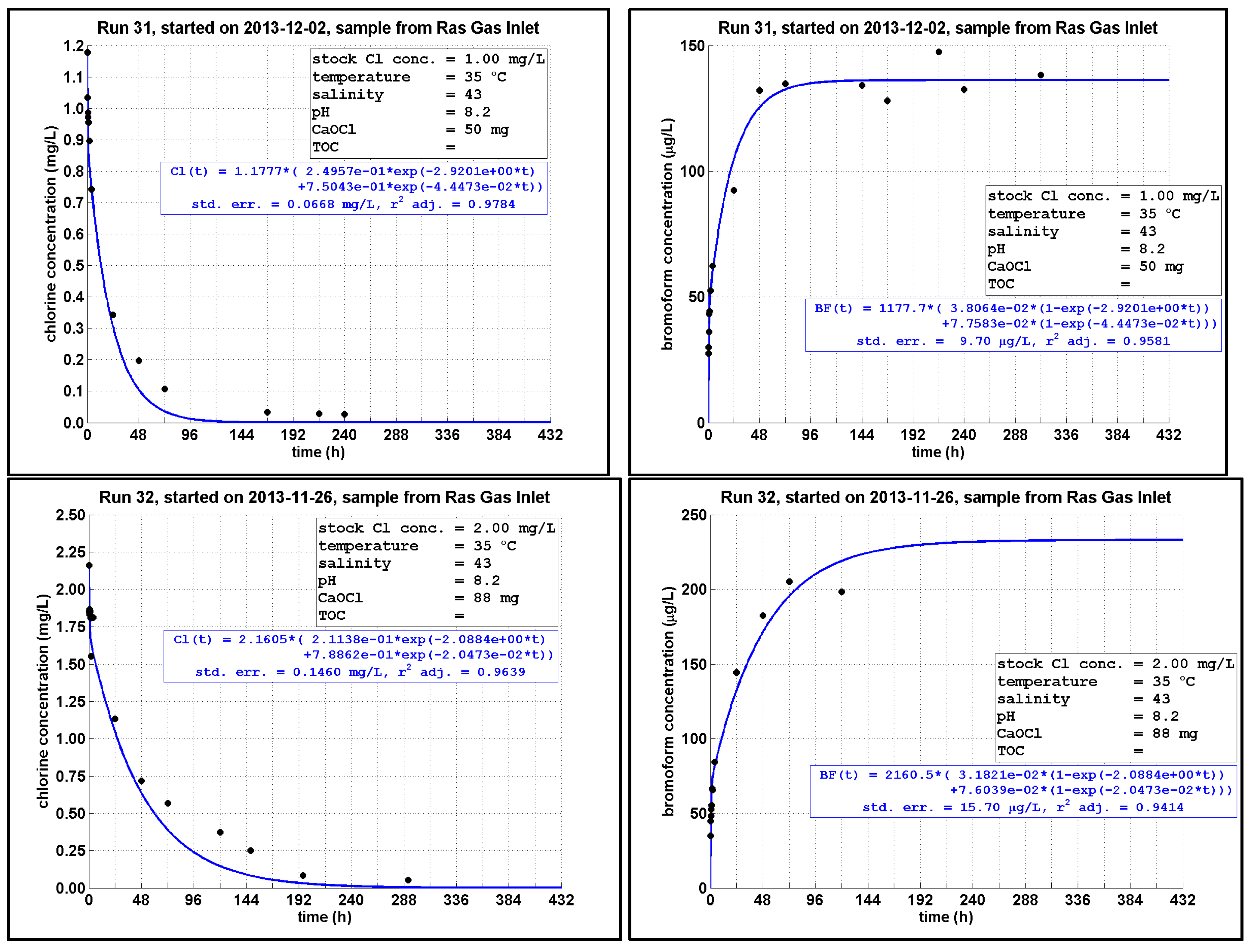
4.4. Chlorine Decay and CBPs Formation with Different Initial Chlorine Dosing Levels

In this study, five initial chlorine concentration settings (0.38, 0.5, 1.0, 2.0 and 5.0 mg/L) were used to examine the effect of initial chlorine concentration on the availability of residual chlorine in seawater. The decay of residual chlorine in seawater with different initial chlorine concentrations is shown in Figure 2. Equation (3) was fit to each time series.

Figure 2. Curve fit results for the effect of initial chlorine concentration on chlorine decay and chlorination by-product (CBP) formation. Insets show run properties and a statistical summary of the curve fit.

Figure 2. Curve fit results for the effect of initial chlorine concentration on chlorine decay and chlorination by-product (CBP) formation. Insets show run properties and a statistical summary of the curve fit.

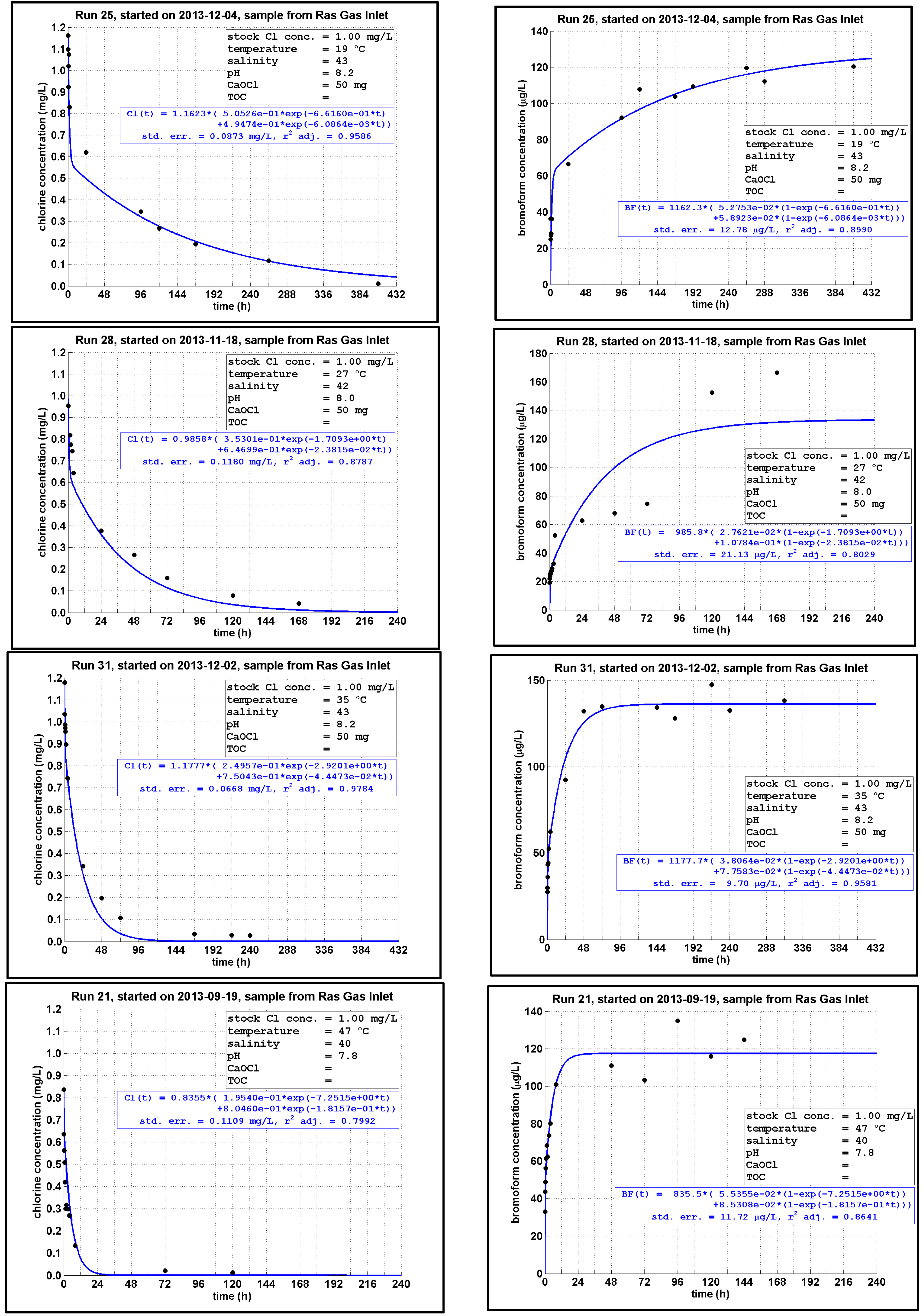
4.5. Chlorine Decay and CBP Formation at Different Temperatures

The level of residual chlorine in seawater is known to be temperature dependent. In this study, five temperature settings (19, 27, 35, 42 and 47 °C) were used to examine the effect of temperature on the change in concentration with the time of residual chlorine in seawater (Figure 3).

Figure 3. Chlorine decay and CBP formation data and fits at different temperatures.

Figure 3. Chlorine decay and CBP formation data and fits at different temperatures.

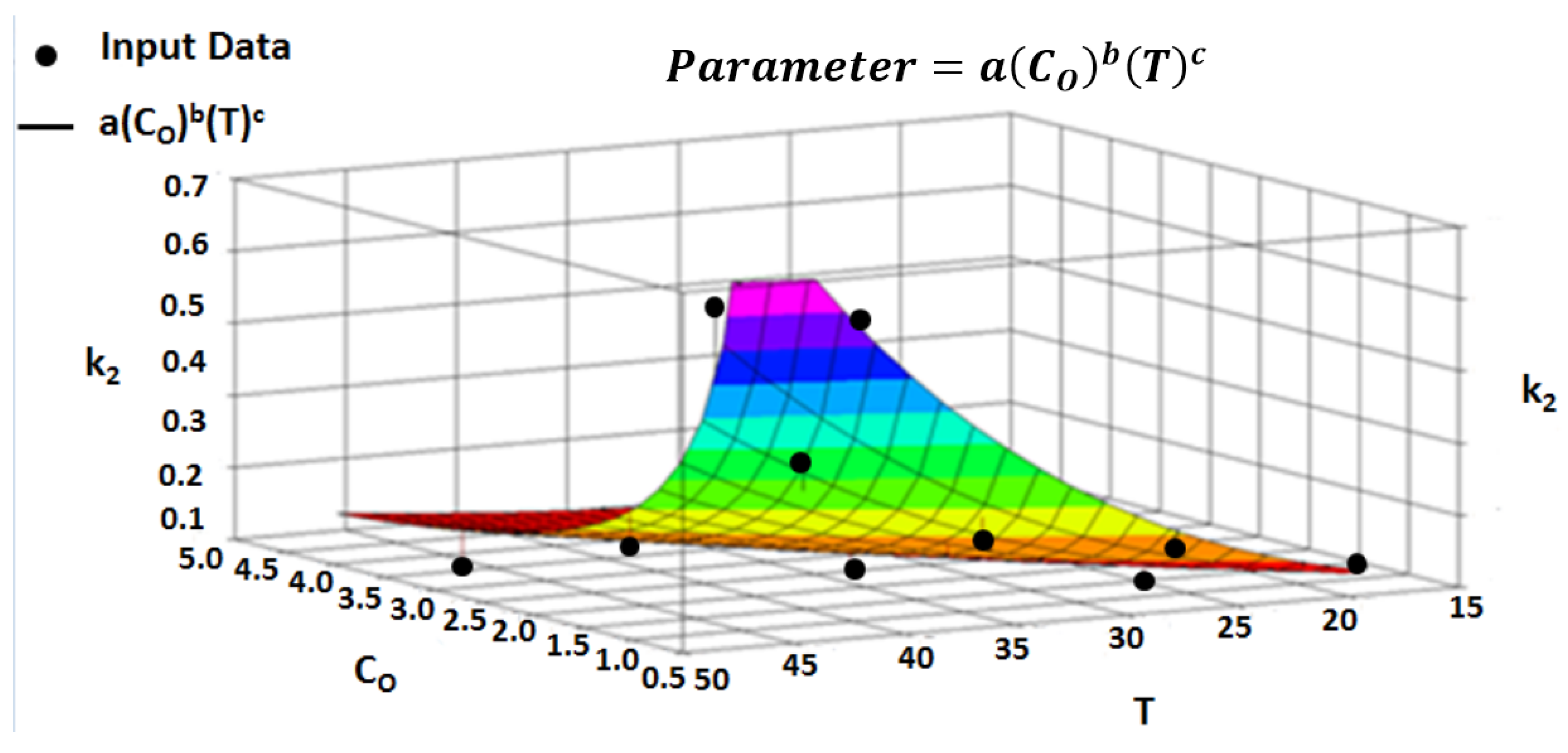
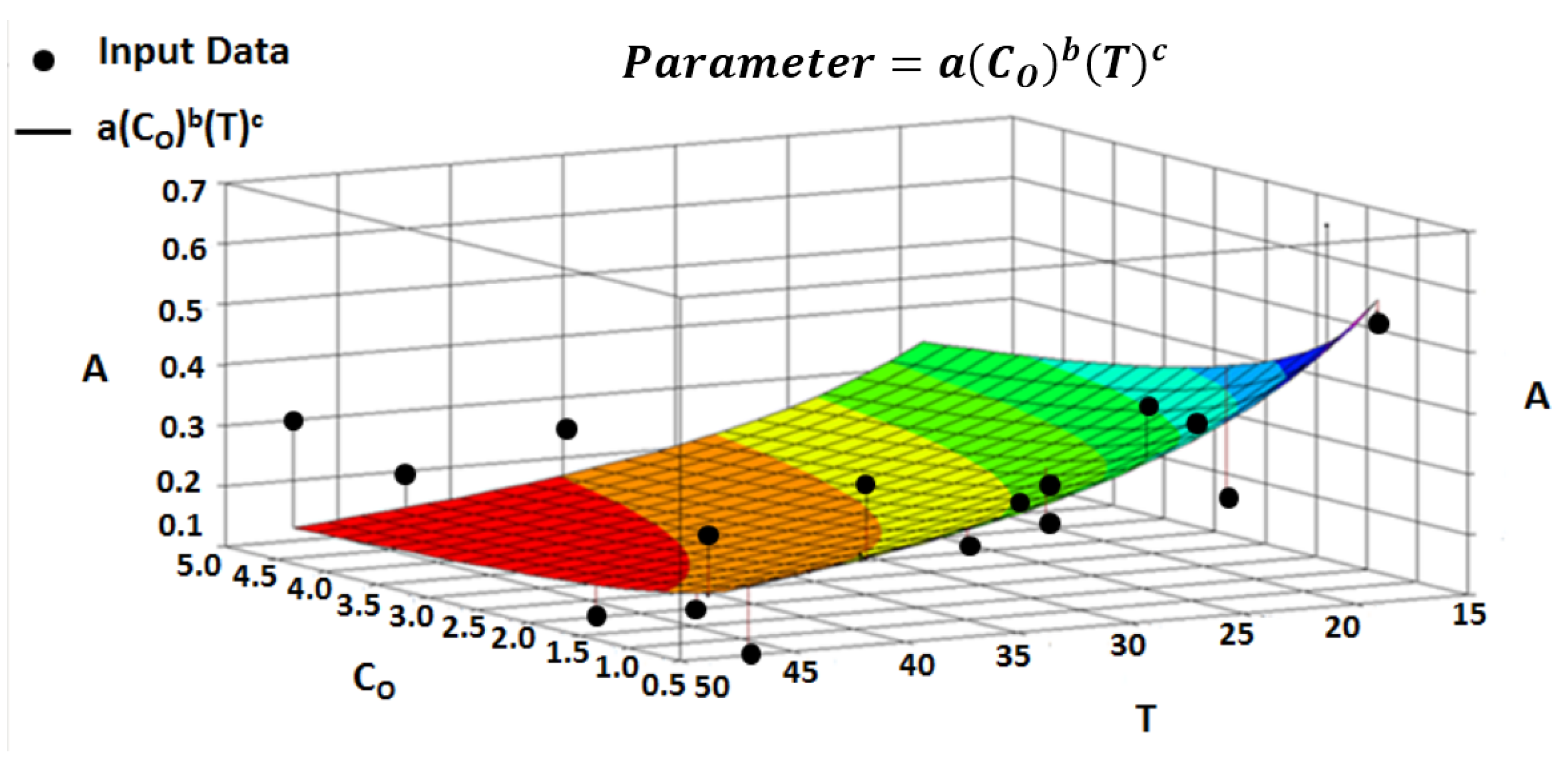
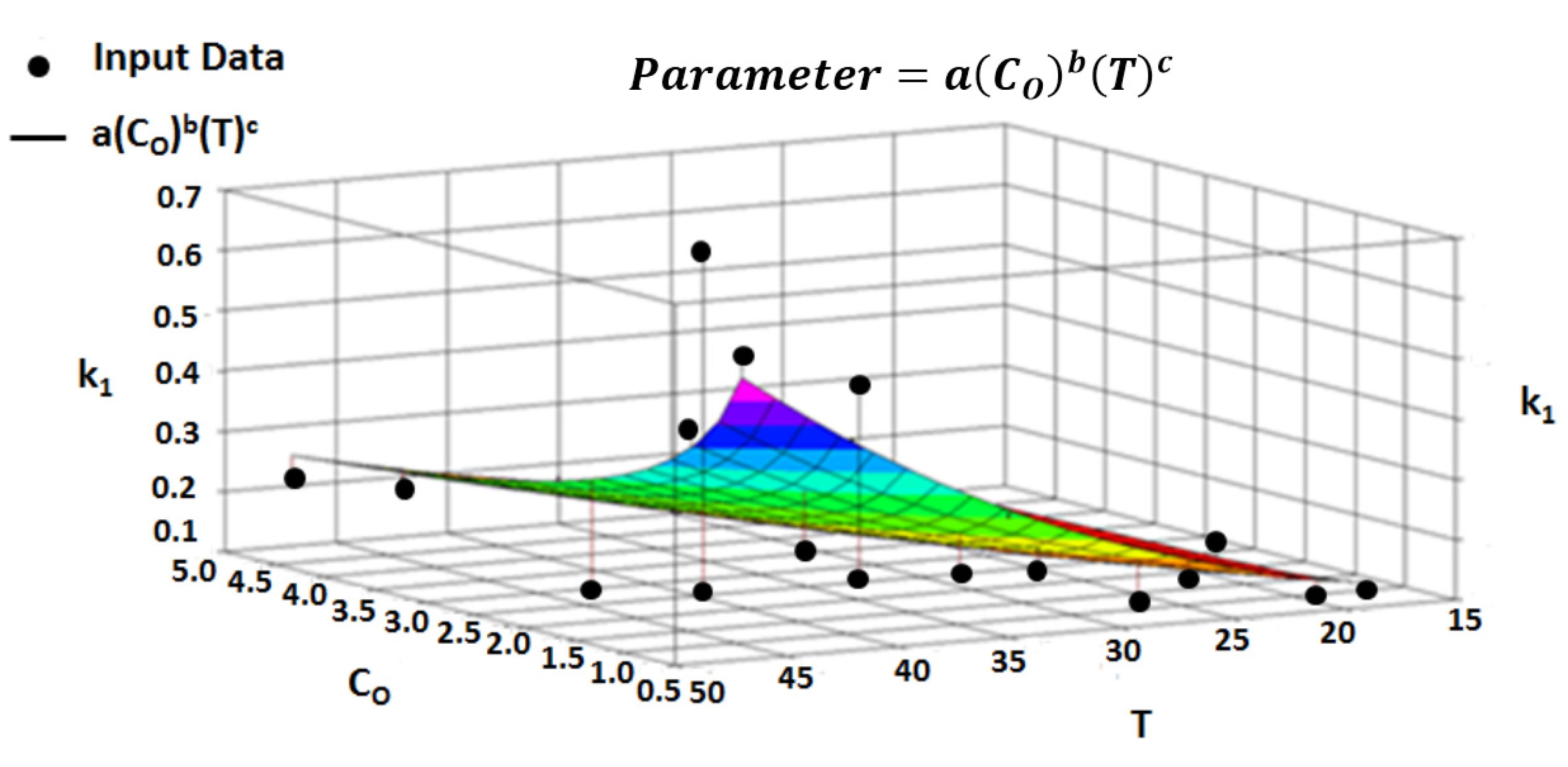
4.6. Multivariate Dependencies

Many studies have identified chlorine dosage, temperature, pH, bromide concentration ($Br$) and natural organic matter ($NOM$) as the most important properties impacting the formation of CBPs [27]. The dependence of parameters $A$, $k_1$ and $k_2$ on these properties and salinity $S$ (potentially important in seawater) is expressed as:

$$\text{parameter}= a{\left(C_0\right)}^b{\left(T\right)}^c{\left(pH\right)}^d{\left(S\right)}^e{\left(Br\right)}^f{\left(NOM\right)}^g$$

(13)

Values for $Br$ and $NOM$ were not available in the present study and, so, are not considered beyond this point. However, as shown below, omitting these variables does not seem to significantly weaken the model.

Prior to performing the multivariate regression analysis, a dependency analysis was performed to understand the dependence of these parameters on the various control parameters. Due to the range of values considered, dependency on the control variables could be evaluated.

The dependence of $A$, $k_1$ and $k_2$ on control variables $C_0$, $T$, $pH$ and $S$ can be evaluated using a graphical approach. Each fit parameter ($A$, $k_1$ or $k_2$) is plotted against each control variable in turn, while holding the other control variables roughly constant. The goal is to extract information regarding the direction and magnitude of the partial derivative, for example, for the dependence of $A$ on $C_0$:

$$A=a{\left(C_0\right)}^b{\left(T\right)}^c{\left(pH\right)}^d{\left(S\right)}^e$$

(14)

$$\frac{\partial A}{\partial C_0}=ab{\left(C_0\right)}^{b-1}{\left(T\right)}^c{\left(pH\right)}^d{\left(S\right)}^e$$

(15)

The ability to determine the dependence on one control variable while holding the others constant is necessarily limited by the set of control variables available in the 25 runs. Therefore, instead of holding each of the other control variables exactly constant, grouping into small reasonable ranges was considered. Desired stock chlorine is used to set up the $C_0$ groups, but the actual $C_0$ values are the ones used in the dependency analysis. The chlorine groups are four equally-sized bins between 0.5 and 5.0 mg/L. The temperature groups are three equally-sized bins between 19 and 47 °C. The pH groups are two equally-sized bins between 7.8 and 8.3. The salinity groups are two equally-sized bins between 40 and 43.

4.7. Multivariate Parameter Equation

How these parameters vary with initial chlorine concentration and temperature was also investigated through multivariate regression. The kinetics of chlorine consumption and by-product formation reactions are known to depend on the initial residual chlorine concentration, pH, salinity, water temperature and the nature and concentration of natural organic matter in the water. The significance of most of these factors on the reaction kinetics was investigated here using the set of laboratory experiments conducted to establish multivariate regression relationships.

The parameters $A$, $A_T$, $B_T$, $k_1$ and $k_2$ are functions of the initial chlorine concentration ($C_0$), temperature ($T$) and $pH$. After estimating the values of these parameters in the curve fitting discussed above, a second and multivariate regression analysis is performed to determine $A$, $A_T$, $B_T$, $k_1$ and $k_2$ as functions of control variables $C_0$, $T$ and $pH$. The general form of the function is:

$$Parameter=a{\left(C_0\right)}^b{\left(T\right)}^c{\left(pH\right)}^d{\left(S\right)}^e$$

(16)

where $a$, $b$, $c$, $d$ and e are obtained from multivariate regression analysis.

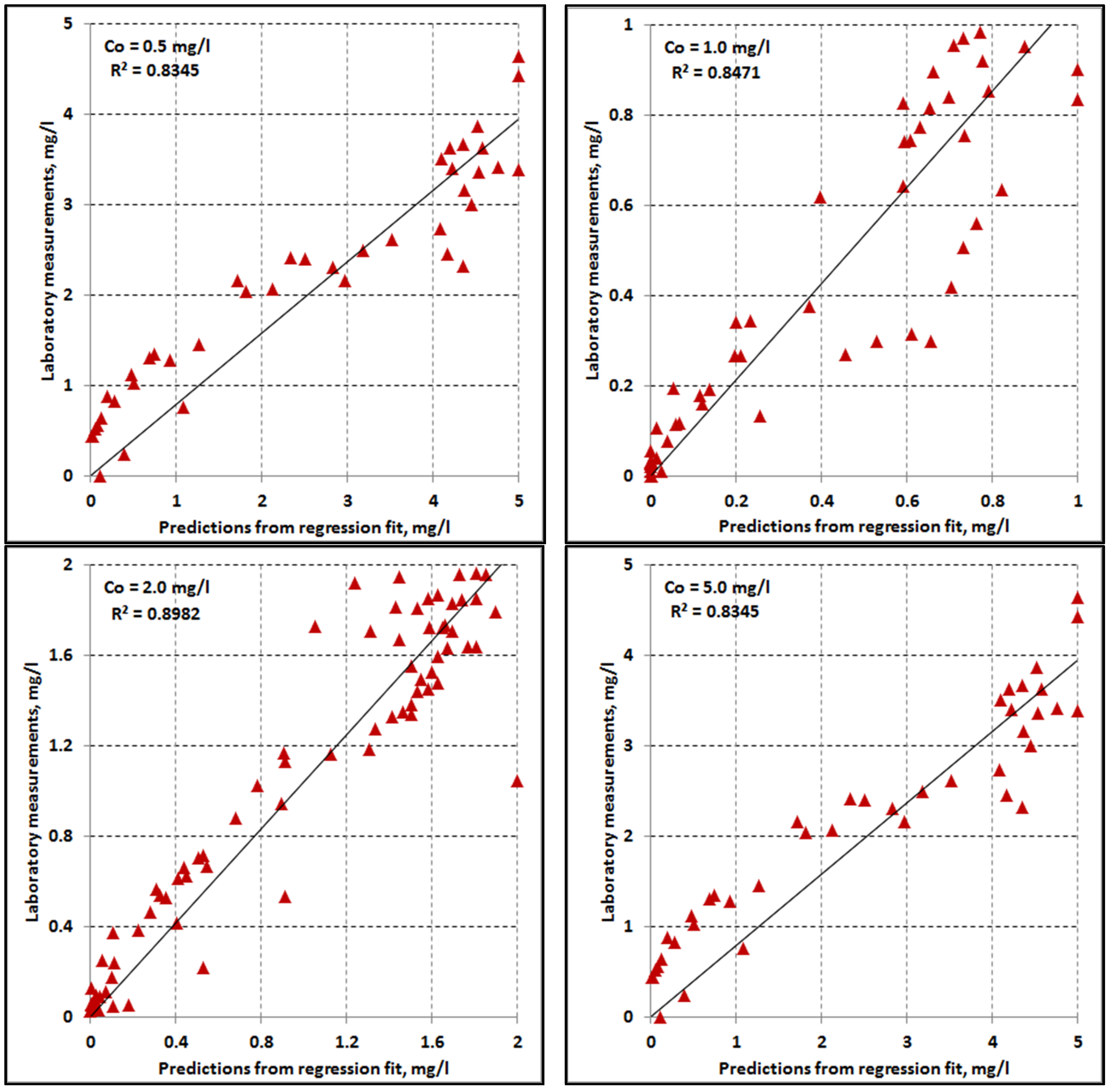
4.8. Multivariate Regression

These analyses represent simplified kinetics for chlorine using regression analyses to find functional relationships between the parameters of the assumed rate equations: $A$, $A_T$, $B_T$, $k_1$ and $k_2$ and the experimental controls $C_0$, $T$ and $pH$. Such functional relationships are required to develop a set of algorithms for describing chlorine transformation in the numerical model.

Based on the results of this dependency analysis, $pH$ and salinity were dropped as control variables due to the fact that these variables do not vary significantly within the seawater samples and also that a consistent dependency could not be determined based on the limited number of runs. Then, Equation (14) reduces to:

$$Parameter=a{\left(C_0\right)}^b{\left(T\right)}^c$$

(17)

Multivariate regression analysis is applied to the chlorine parameters, and the resulting values for $a$, $b$ and $c$ are summarized in Table 1. The multivariate functions for $A$, $k_1$ and $k_2$ are shown in Figure 4, Figure 5 and Figure 6, respectively. For brevity, these figures are only shown for chlorine and not for CBPs.

Figure 4. Multivariate function resulting from regression for chlorine parameter $A$.

Figure 4. Multivariate function resulting from regression for chlorine parameter $A$.

Figure 5. Multivariate function resulting from regression for chlorine parameter $k_1$.

Figure 5. Multivariate function resulting from regression for chlorine parameter $k_1$.

Figure 6. Multivariate function resulting from regression for chlorine parameter $k_2$.

Figure 6. Multivariate function resulting from regression for chlorine parameter $k_2$.

Table 1. Coefficient and exponents obtained for chlorine using multivariate regression analysis.

Parameter	$\text{Parameter}=a{\left(C_0\right)}^b{\left(T\right)}^c$
	$a$	$b$	$c$
$A$	1.550 × 101	−2.737 × 10−1	−1.149 × 100
$k_1$ (h−1)	5.416 × 10−4	−5.524 × 10−1	2.442 × 100
$k_2$ (h−1)	4.612 × 10−7	−1.277 × 100	3.287 × 100

Table 1. Coefficient and exponents obtained for chlorine using multivariate regression analysis.

Parameter	$\text{Parameter}=a{\left(C_0\right)}^b{\left(T\right)}^c$
	$a$	$b$	$c$
$A$	1.550 × 101	−2.737 × 10−1	−1.149 × 100
$k_1$ (h−1)	5.416 × 10−4	−5.524 × 10−1	2.442 × 100
$k_2$ (h−1)	4.612 × 10−7	−1.277 × 100	3.287 × 100

Similar multivariate regression analysis can be done for the CBPs. Bromoform was reported in 19 of 25 runs and is one of the major CBPs produced as chlorine is consumed. In contrast, BDCM and DBCM were only reported in 7 and 12 runs, respectively. Because the number of laboratory runs for BDCM and DBCM is insufficient and because bromoform is a major concern, the only CBP to which the multivariate regression analysis is applied is bromoform. Table 2 summarizes the results of the multivariate regression analysis for bromoform.

The correlation between laboratory measurements and multivariate regression (with coefficients and exponents listed in Table 1) -predicted chlorine concentrations are shown in Figure 7 for different initial chlorine dosages and for all temperature settings. The value of R² is 0.83 for C₀ = 0.5 mg/L, 0.85 for C₀ = 1.0 mg/L, 0.90 for C₀ = 2.0 mg/L and 0.83 for C₀ = 5.0 mg/L.

The correlation between laboratory measurements and multivariate regression (with coefficients and exponents listed in Table 2) -predicted bromoform concentrations are shown in Figure 8, for different initial chlorine dosages and for all temperature settings. The value of R² is 0.84 for C₀ = 0.5 mg/L, 0.79 for C₀ = 1.0 mg/L, 0.92 for C₀ = 2.0 mg/L and 0.77 for C₀ = 5.0 mg/L.

Table 2. Coefficients obtained for bromoform using multivariate regression analysis.

parameter	$\text{parameter}=a{\left(C_0\right)}^b{\left(T\right)}^c$
	$a$	$b$	$c$
$A_T$	1.090 × 10−1	−6.932 × 10−1	−2.330 × 10−1
$B_T$	2.872 × 10−3	1.965 × 10−1	8.955 × 10−1

Table 2. Coefficients obtained for bromoform using multivariate regression analysis.

parameter	$\text{parameter}=a{\left(C_0\right)}^b{\left(T\right)}^c$
	$a$	$b$	$c$
$A_T$	1.090 × 10−1	−6.932 × 10−1	−2.330 × 10−1
$B_T$	2.872 × 10−3	1.965 × 10−1	8.955 × 10−1

Figure 7. Correlation between observed and multivariate regression predicted chlorine decay at different chlorine dosages for all temperature settings.

Figure 7. Correlation between observed and multivariate regression predicted chlorine decay at different chlorine dosages for all temperature settings.

The relative errors between the predicted value and real determination were practically acceptable based on R² values and considering uncertainties associated with laboratory sampling analysis. Therefore, this prediction model would be applicable to industrial plants that access seawater with properties similar to those described above.

4.9. Effect of Water Composition

The characterization of seawater collected from the inlet of cooling seawater in RLC industrial plants in Qatar indicated that the pH was between 7.8 and 8.3, salinity between 40 psu and 43 psu and TOC between 1.9 and 2.4 mg/L. As discussed above, the predictive power of the model appears to be relatively independent of these variables, which is not surprising given their narrow range of variability at this site.

Figure 8. Correlation between laboratory measurements and multivariate regression predicted bromoform formation at different chlorine dosages for all temperature settings.

Figure 8. Correlation between laboratory measurements and multivariate regression predicted bromoform formation at different chlorine dosages for all temperature settings.

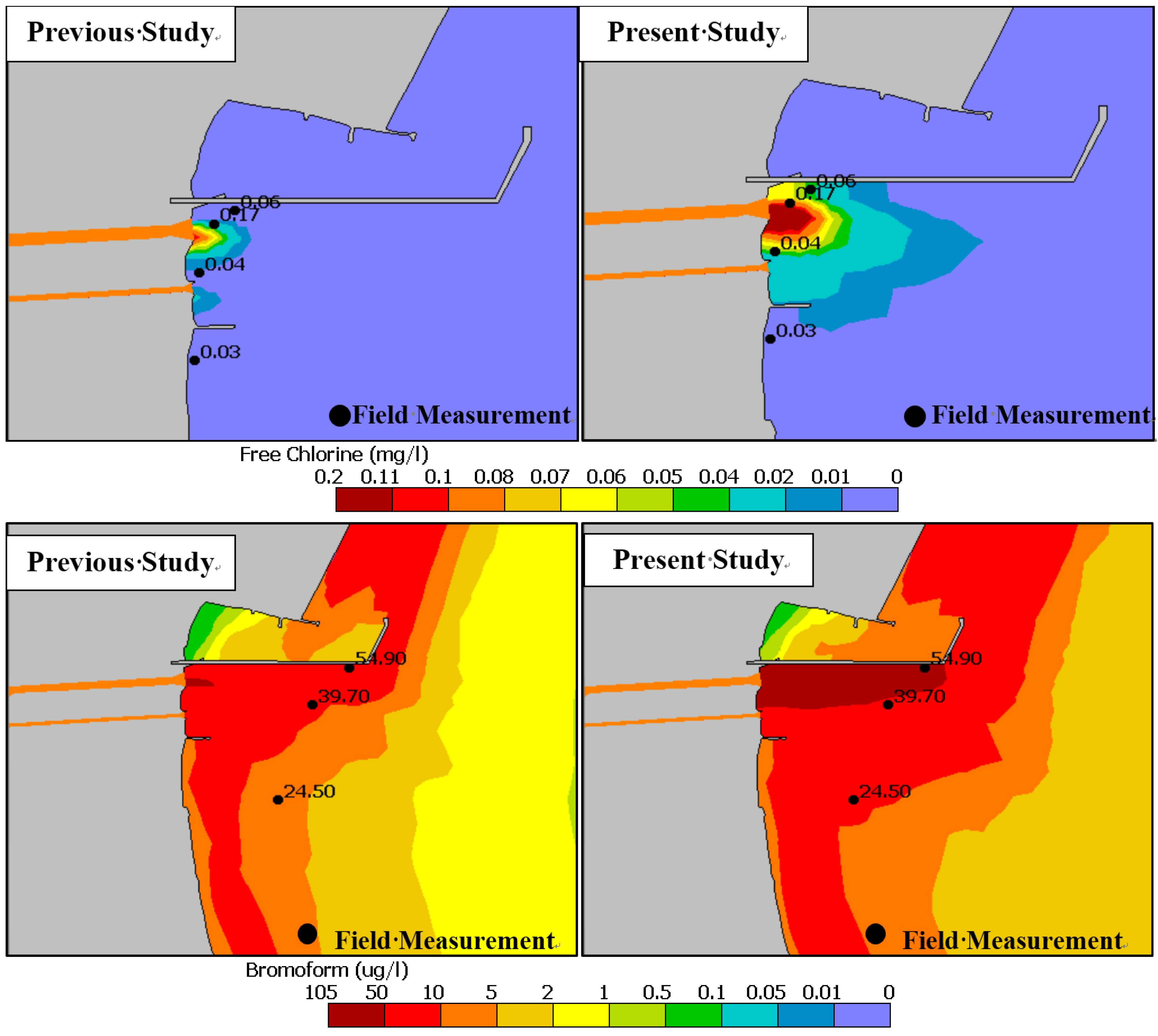
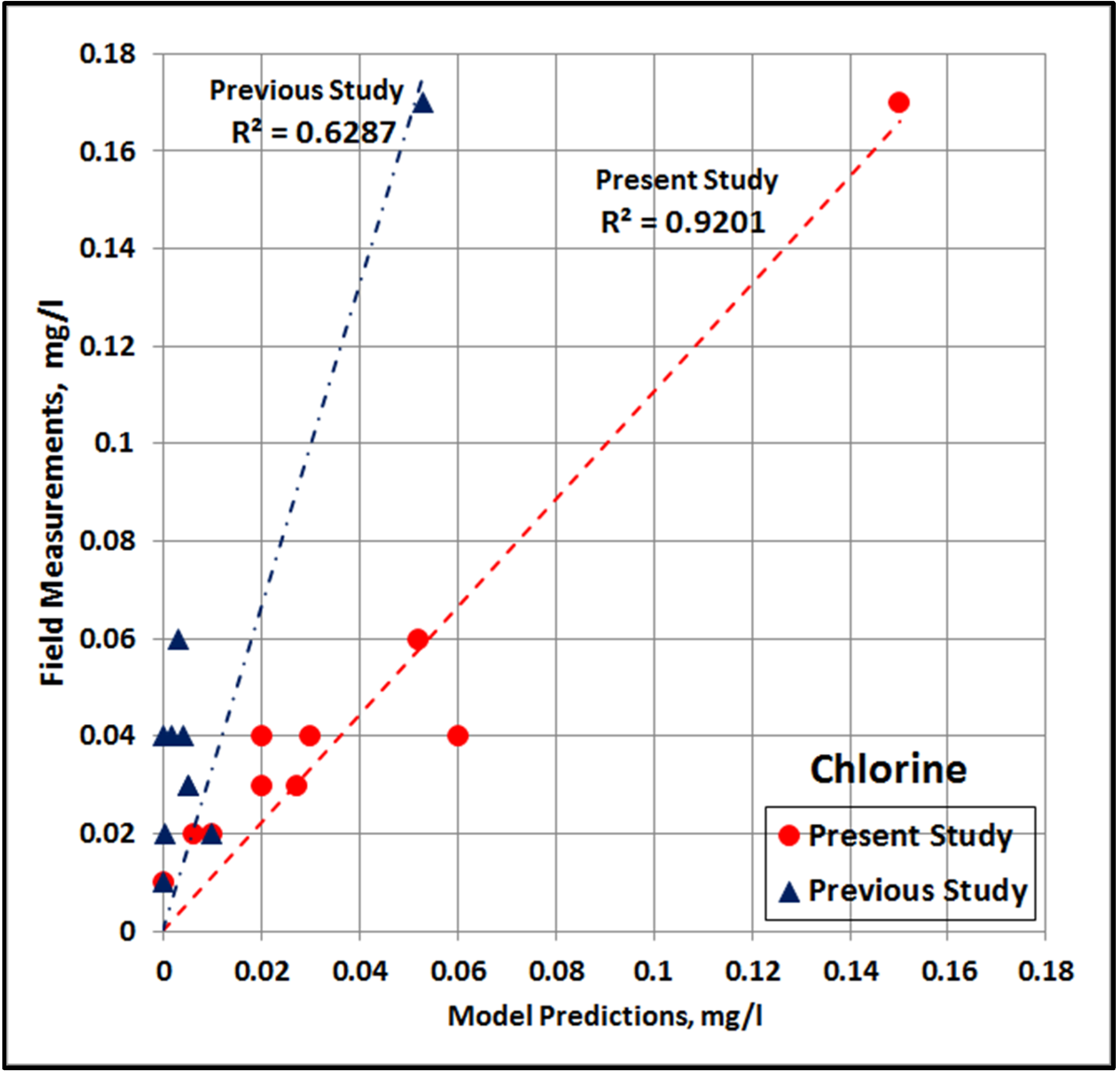
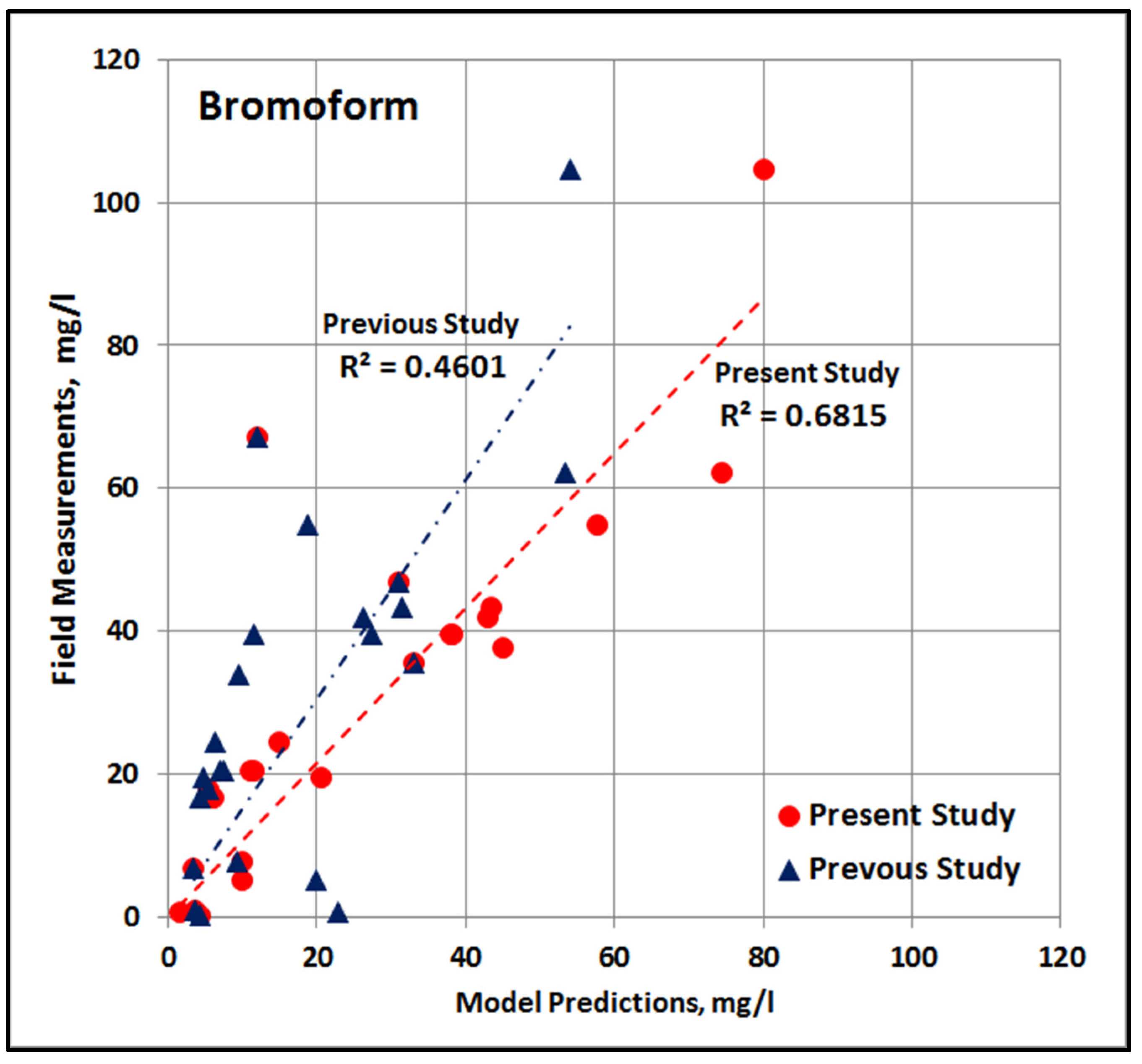
4.10. Comparison with Previous Study

The goal of the existing study is to improve upon the previously-developed relationships. As such, the performance of these chlorine decay and CBPs formation relationships was compared against the previous field study from the year 2006 (9 and 10). The contour plot of GEMSS model predicted residual chlorine concentrations in the vicinity of RLIC outfall using previously developed relationships and with the updated relationships in the vicinity of RLIC outfall during a typical flood tide stage is shown in Figure 9. Field measurements during this time are also shown in the same figure. Figure 9 clearly shows that the model-predicted results using the updated chlorine decay relationship improve the predictability when compared with the field measurements. In the same figure, the model-predicted bromoform concentrations using the new CBP formation relationship are shown, which also compare reasonably well with the field measurements for the same tide stage.

Figure 9. Correlation between laboratory measurements and multivariate regression-predicted bromoform formation at different chlorine dosages for all temperature settings.

Figure 9. Correlation between laboratory measurements and multivariate regression-predicted bromoform formation at different chlorine dosages for all temperature settings.

The results shown in Figure 9 illustrate model-field comparison only for one tide stage. However, several field measurements were conducted for other tidal stages during the year 2006 [9,10]. Therefore, in order to perform a more comprehensive comparison of these results, GEMSS results and the corresponding field measurements were plotted in Figure 10 and Figure 11 in a more summarized fashion. The model predictions are much closer to field measurements in the case of new relationships when compared with previous relationships. Model predictability has significantly improved across the various tidal conditions for both chlorine and bromoform. The updated relationships have a 0.92 for R², while the previous relationships had a 0.63 for R². These results clearly show that the new relationships are able to support the validity of the GEMSS-CKM model and significantly improve the model’s predictability for a real-world case.

The present study has some significant improvements over the previous study:

• Actual intake water was used, resulting in chlorination of water that consisted of NOM representative of the ambient RLIC waters.
• Use of the actual intake water indicated the small variability of pH and salinity. This resulted in exclusion of pH and salinity as control variables.
• In the present study, a range of 19–47 °C was used for temperature and a range of 0.38–5.00 mg/L was used for chlorine dosage. These wider ranges were more representative of actual operations and site-specific ambient conditions, which helps cover all possibilities for the predominant control variables, resulting in improved analysis.
• Each lab run was done so that better temporal resolution was achieved during the early parts of the run with measurements every 15 min for the first hour and every 30 min for the next hour. This higher resolution provided additional data to help with studying the fast reaction after the initial dosing.
• Each lab run was also run for a much longer time during the present study, which assured increased data during the latter part of the run when the slow reaction is dominant. Data during the slow reaction is crucial, as the water dosed with chlorine enters the RLIC water during this period. It is highly important to put more emphasis on the slow reaction phase, as the interaction with NOM in the ambient water and the resulting environmental impacts would occur during this period.
• The increased number of data during the slow reaction phase ($k_2$) provided increased quality of fit during this phase. Due to the longer period, the quality of fit could be evaluated for up to several days, as compared to the previous relationships.

Figure 10. Comparison of GEMSS model predictions vs. field measurements for previous and present study chlorine decay rate regressions.

Figure 10. Comparison of GEMSS model predictions vs. field measurements for previous and present study chlorine decay rate regressions.

Figure 11. Comparison of GEMSS model predictions vs. field measurements for previous and present study bromoform formation rate regressions.

Figure 11. Comparison of GEMSS model predictions vs. field measurements for previous and present study bromoform formation rate regressions.

5. Conclusions

Use of chlorination as a method to avoid biofouling is a common practice globally. Some environmental concerns exist where the residual chlorine can react with the NOM of the ambient water to produce CBPs. The study described in this article discusses a field and laboratory study designed to develop a mathematical model capable of predicting residual chlorine and resulting CBP fate and transport. A generic mathematical model is introduced, which, then, is further customized to provide site-specific predictive capabilities.

The article provides a demonstration application where a comprehensive set of laboratory experiments were used to parameterize mathematical models capable of predicting chlorine and CBP fate. Since the study was built on a previous study, several improvements were outlined as identified from experience gained from site-specific application. The results from this study showed that only some of the control parameters identified in the literature were important for predicting residual chlorine and CBP concentrations for this specific location. Initial chlorine concentration and temperature were identified to be important parameters, while pH, salinity and initial TOC concentration were found as independent variables due to them being almost constant at this site. Although further enhancements and steps have been identified within this article, the study demonstrates a comprehensive and flexible framework of laboratory procedures and mathematical modeling that can be applied worldwide for predictive chlorine and CBP modeling. This framework can be further enhanced to work with exposure models for environmental impact assessments to sensitive receptors.

Furthermore, this predictive model could also be used in the design of cooling systems with known general conditions and an established median lethal concentration (LC₅₀) for local marine organisms. Safe concentrations of chlorine dosage and discharge can be calculated as part of cooling system designs. If the criteria for residual chlorine discharging into ambient seawater are determined, the optimal chlorine concentration for a cooling system can be calculated by measuring residual chlorine in the system and knowing the cooling pipeline length.

References

- Wong, G.T.F.; Davidson, J.A. The fate of chlorine in seawater. Water Res. 1977, 11, 971–978. [Google Scholar] [CrossRef]
- Stanbro, W.D. The Chemistry of Power Plant Chlorination; John Hopkins University, Applied Physics Laboratory: Laurel, MD, USA, 1983; pp. 1–25. [Google Scholar]
- Shames Al-Din, A.M.; Arain, A.M.; Hammoud, A.A. On the chlorination of seawater. Desalination 2000, 129, 53–62. [Google Scholar] [CrossRef]
- Fayad, N.M.; Iqbal, S. Chlorination by-products of Arabian Gulf seawater. Bull. Environ. Contam. Toxicol. 1987, 78, 475–482. [Google Scholar] [CrossRef]
- Shames Al-Din, A.M.; Arain, A.M.; Hammoud, A.A. A contribution to the problem of trihalomethane formation from the Arabian Gulf water. Desalination 1991, 85, 13–32. [Google Scholar] [CrossRef]
- Abdel-Wahab, A.; Khodoury, A.; Bensalah, N. Formation of trihalomethanes during seawater chlorination. J. Environ. Pollut. 2010, 1, 456–465. [Google Scholar] [CrossRef]
- Eppley, R.W.; Roger, E.H.; Williams, P.M. Chlorine reaction with seawater constituents and the inhibition of photosynthesis of natural phytoplankton. Estuar. Coast. Mar. Sci. 1976, 4, 147–161. [Google Scholar] [CrossRef]
- Agus, A.; Koutchkov, N.; Sedlak, D. Disinfection by-products and their potential impact on the quality of water produced by desalination systems: A literature review. Desalination 2009, 237, 214–237. [Google Scholar] [CrossRef]
- Adenekan, A.E.; Kolluru, V.S.; Smith, J.P. Transport and fate of chlorinated by-products associated with cooling water discharges. In Proceedings of the 1st Annual Gas Processing Symposium; Alfadala, H., Rex Reklaitis, G.V., El-Halwagi, M.M., Eds.; Elsevier: Berlin, Germany, 2009. [Google Scholar]
- Febbo, E.; Kolluru, V.S.; Prakash, S. Numerical Modeling of Thermal Plume and Residual Chlorine Fate in Coastal Waters of the Arabian Gulf. In Proceedings of the SPE/APPEA International Conference on Health, Safety, and Environment in Oil and Gas Exploration and Production, Perth, Australia, 11–13 September 2012.
- Saeed, S.; Deba, N.; Campbell, R.; Kolluru, V.S.; Prakash, S.; Febbo, E. Cooling Water Discharge to the Qatar Marine Zone-Laboratory Determination of Chlorine Decay Kinetics as Input to Numerical Fate and Transport Model; Qatar Foundation Research Forum: Doha, Qatar, 2013. [Google Scholar]
- Rook, J.J. Chlorination reactions of fulvic acids in natural waters. Environ. Sci. Techol. 1977, 11, 478–482. [Google Scholar] [CrossRef]
- Clark, R.M.; Sivaganesan, M. Predicting chlorine residual and formation of TTHMs in drinking water. J. Environ. Eng. 1998, 124, 1203–1210. [Google Scholar] [CrossRef]
- Chowdhury, S.; Champagne, P. An Investigation on Parameter for Modeling THMs Formation. Glob. NEST J. 2008, 10, 80–91. [Google Scholar]
- Haas, C.N.; Karra, S.B. Kinetics of wastewater chlorine demand exertion. J. Water Pollut. Control Fed. 1984, 56, 170–173. [Google Scholar]
- Sohn, J.; Amy, G.; Cho, J.; Lee, Y.; Yoon, Y. Disinfectant decay and disinfection by-products formation model development: Chlorination and ozonation by-products. Water Res. 2004, 38, 2461–2478. [Google Scholar] [CrossRef] [PubMed]
- Fabbrincino, M.; Korshin, C.V. Modeling disinfection by-product formation in bromide containing water. J. Hazard. Mater. 2009, 168, 782–786. [Google Scholar] [CrossRef] [PubMed]
- Hua, F.; West, J.R.; Barker, R.A.; Forster, C.F. Modelling of chlorine decay in municipal water supplies. Water Res. 1999, 33, 2735–2746. [Google Scholar] [CrossRef]
- Clark, R.M. Chlorine demand and TTHM formation kinetics: A second-order model. J. Environ. Eng. 1998, 124, 16–24. [Google Scholar] [CrossRef]
- Jadas-Hécart, A.; El Morer, A.; Stitou, M.; Bouillot, P.; Legube, B. Chlorine demand of a treated water [Modelisation de la demande en chlore d’une eau traitee]. Water Res. 1992, 26, 1073–1084. [Google Scholar] [CrossRef]
- Ventresque, C.; Bablon, G.; Legube, B.; Jadas-Hécart, A.; Dore, M. Development of chlorine demand kinetics in a drinking water treatment plant. Water Chlorination Chem. Environ. Impact Health Eff. 1990, 6, 715–728. [Google Scholar]
- Saeed, S.; Deba, N.; Cambell, R.; Prakash, S.; Kolluru, V.S. Laboratory experiments to validate 3D numerical modeling of chlorine decay in industrial cooling water discharge. In Proceedings of the Society of Environmental Toxicology and Chemistry (SETAC) Europe 23rd Annual Meeting: Building a Better Future: Responsible Innovation and Environmental Protection, Glasgow, UK, 12–16 May 2013.
- Kolluru, V.; Prakash, S.; Febbo, E. Modeling the Fate and Transport of Residual Chlorine and Chlorine By-Products (CBP) in Coastal Waters of the Arabian Gulf. In Environmental Science and Technology, Proceedings of the Fifth International Conference on Environmental Science and Technology, Houston, TX, USA, 25–29 June 2012; Sorial, G.A., Hong, J., Eds.; American Science Press: Houston, TX, USA, 2012; pp. 385–391. [Google Scholar]
- HACH. AutoCATTM9000 Amperometric Titrator User Manual for Chlorine, Chlorine Dioxide, Chlorite, Sulfite and Total Oxidants; HACH: Loveland, CO, USA, 2007. [Google Scholar]
- Stock, J.T. Amperometric Titrations. Anal. Chem. 1972, 44, 1–9. [Google Scholar] [CrossRef] [PubMed]
- Chang, E.E.; Chang, P.C.; Chao, S.H.; Lin, Y.L. Relationship between chlorine consumption and chlorination by-products. Chemosphere 2009, 64, 1196–1203. [Google Scholar] [CrossRef] [PubMed]
- Buttrick, D.; Tobiason, J.E.; Ahlfeld, D.P. Modeling as an Operational Tool for an Unfiltered Surface Water Supply. In Proceedings of the American Water Works Association Annual Conference, San Francisco, CA, USA, 12–16 June 2005.
© 2015 by the authors; licensee MDPI, Basel, Switzerland. This article is an open access article distributed under the terms and conditions of the Creative Commons Attribution license ( http://creativecommons.org/licenses/by/4.0/).
Share and Cite
Saeed, S.; Prakash, S.; Deb, N.; Campbell, R.; Kolluru, V.; Febbo, E.; Dupont, J. Development of a Site-Specific Kinetic Model for Chlorine Decay and the Formation of Chlorination By-Products in Seawater. J. Mar. Sci. Eng. 2015, 3, 772-792. https://doi.org/10.3390/jmse3030772
Saeed S, Prakash S, Deb N, Campbell R, Kolluru V, Febbo E, Dupont J. Development of a Site-Specific Kinetic Model for Chlorine Decay and the Formation of Chlorination By-Products in Seawater. Journal of Marine Science and Engineering. 2015; 3(3):772-792. https://doi.org/10.3390/jmse3030772
Chicago/Turabian StyleSaeed, Suhur, Shwet Prakash, Nandita Deb, Ross Campbell, Venkat Kolluru, Eric Febbo, and Jennifer Dupont. 2015. "Development of a Site-Specific Kinetic Model for Chlorine Decay and the Formation of Chlorination By-Products in Seawater" Journal of Marine Science and Engineering 3, no. 3: 772-792. https://doi.org/10.3390/jmse3030772