In this study, we analyzed the South Atlantic States region due to its unique geographical settings. With more than one thousand miles of coastline, the South Atlantic States region mainly consists of Florida, Georgia, North Carolina, and South Carolina. Nevertheless, in the past decades, as the sea surface temperature has risen, the power of Atlantic tropical cyclones has risen dramatically [
18,
19] and made this region particularly vulnerable to extreme weather events. During the extremely active 2017 Atlantic Basin hurricane season, 17 named tropical cyclones (of which six became major hurricanes) and two weaker systems developed from April to early November [
20]. It was one of the most destructive hurricane seasons in history, costing more than
$250 billion in damage alone in the U.S. [
21]. To demonstrate the performance of our model, we used the AIS data of the Universal Transverse Mercator (UTM) Zone 17 dataset of 2017. This dataset is provided by marine cadaster [
22], which are mainly located in the South Atlantic States region. These regions are featured with their high density of ship flows (more detail on the selection procedure is provided in
Section 3.1.1). As the original datasets do not explicitly define the boundaries of zones, we used hexagons to partition and group ship flow data for the following reasons. First, no widely-accepted boundary partition mechanism is available for this region. Second, hexagons can better support algorithmic efficiency, data representation, and semantic expressiveness [
23,
24]. To examine the impacts of hurricanes, we reconstructed the paths and impacted regions of hurricanes using the data from the National Oceanic and Atmospheric Administration Hurricane Center [
25].
To generate spatially continuous hexagons, we used Uber’s H3 hexagonal hierarchical spatial indexing (H3) grid system [
26]. The H3 grid system developed by Uber is originally used for ride optimization, spatial data visualization, and data exploration. The H3 system can be used to group geolocation data points into hexagonal areas or cells. Furthermore, this H3 system supports 16 different resolutions to group data at different spatial scales. There is also a hierarchical relationship for cells at different resolutions. The smaller hexagonal cell (child cell) with a finer resolution is approximately one seventh of the area of its hexagonal cell (parent cell) with coarser resolution. Furthermore, since each of the H3 cells has a unique identifier, it is easy for a child cell to locate its parent cell at coarser resolution and identify the unambiguous neighboring hexagons with the same resolution based on a specific search radius. This efficient indexing system allows us to group and search hexagonally grouped data in an efficient manner to analyze the pattern of ship flow. We only used level 3 and 4 hexagons because these are reasonable sizes for traffic flow management in the coastal waters. Hexagons with coarser resolution cover much greater regions (e.g., states or nations) where prediction results can be less meaningful, whereas hexagons with finer resolution only cover smaller regions where there are only a few ships. For instance,
Figure 1 shows the 11 hexagons considered as ROIs at level 3 for the case studies, which included four regions for the hourly prediction test and one region for the hurricane impact test. The details on selecting these regions are described in
Section 3.1.1. We prepared two sets of ship flow data using different hexagon sizes (
Table 1) based on the processing procedures as explained in the following sections.
3.1. Traffic Flow Analysis
Before formulating a prediction method, we examined the typical spatiotemporal factors in determining the traffic flow in ROI regions. The classic ship traffic simulation contains both micro (focusing on the performance of the individual ship’s navigation) and macro models (treat vessel traffic flow as a whole) based on the ‘Network Simulation’ of nodes and lines [
27]. Our method was adapted from the macro method by considering the relative motions and distributions of ships. According to Xie and Liu (2018), traffic flow usually exhibits temporal regularity except for special conditions such as flooding events, hurricane seasons, and regulations. Furthermore, as ships move across different regions, the spatial association among regions can also alter the level of traffic flow. Therefore, we performed the pattern analysis outlined below to verify the impacts of typical spatiotemporal factors in contributing to the flow level. The pattern analysis serves as the basis of understanding the changes in traffic flow and the model formulation. In the context of this work, for a given hexagon cell, we defined the two types of ship traffic volume as follows: (1) ship flow in same direction where the total number of ships that move from each of the adjacent surrounding hexagons toward the center hexagon within the given interval of time (e.g., one hour or one day); and (2) the total ship flow where the total number ships with a unique identification is located within each of the hexagons within the given interval of tie.
Below, we explain the analysis methods and use our case study region as an example to assess the impacts of different factors. We recognize that the impacts of different factors may change over regions. When performing predictions, our data-driven machine learning model automatically adjusted the weight of factors based on the data in the South Atlantic States region.
3.1.1. ROI Identification
In order to extract high density regions, we used the ship tracking points to reconstruct the ship trajectories to calculate (1) the track point-based density and (2) the track line-based density by assigning points and line segments to grids (
Figure 2). Then, we performed reclassification based on the density threshold to identify high density cells as ROIs in the South Atlantic States region. After we identified the ROIs, we used the honeycomb model for spatiotemporal partitions to generate dynamic models [
23]. Finally, we selected level 3 and level 4 hexagons that overlapped with high density regions and identified them as the final ROIs for ship flow analysis (
Figure 1 and
Table 1).
3.1.2. Spatial Distribution of Traffic Flow
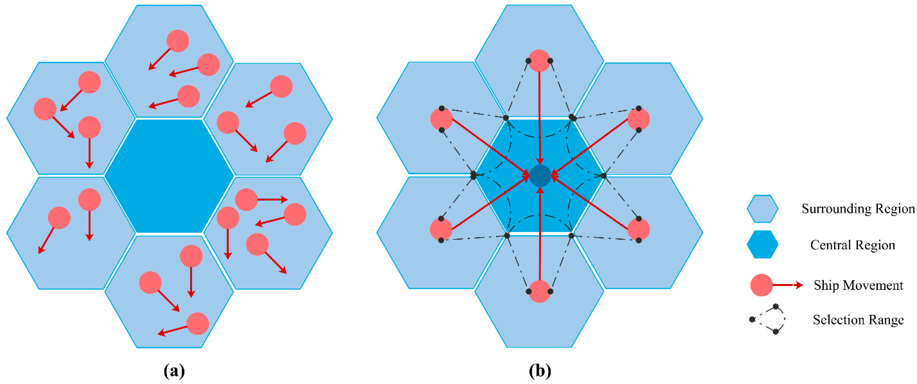
We developed two ways to identify ship flow in the surrounding regions. For the first method, we simply calculated the total number of ships in each of the surrounding hexagons (
Figure 3a). For the second method, we calculated the total number of ships moving toward the central hexagon (
Figure 3b). In order to select the ships moving toward the central zone, we (1) calculated the compass bearing between the center of the of the surrounding H3 zone and the central H3 zone; (2) calculated the compass bearing between the start and end point of the ship; and (3) calculated the absolute difference between the bearings to select ships with bearing differences smaller than 30 degrees. The second method is more ideal for hourly prediction since ships may have moved across several hexagonal zones, covered longer distances, and show more complicated moving patterns at a daily level.
To measure the spatial association, we used local indicators of spatial association (LISA) to explore the degree of spatial autocorrelation [
28] at each unique location based on the local Moran’s I. This can help us find clusters based on each zone’s ship flow values. The local Moran’s I is calculated as follows:
where n is the total number of features;
is the attribute of feature
I; the average of the corresponding attribute is
; and the spatial weight between
i and
j.
For each of the hexagons identified based on ROIs, we performed the following analysis to explore the clustering pattern as the distance of the adjacent hexagons from the central hexagon increased. We first identified hexagons at level 3 that intersected with the ROIs and selected the neighboring hexagons with the same resolution based on the H3’s traverse function with a distance of five.
Figure 4 shows an example of all the neighboring hexagons selected based on the central hexagon (zone l3_Z2). Then, we calculated the total amount of ship flow in each of the hexagons. Based on the ship flow information, we analyzed the hexagons’ clustering pattern using LISA. The result of the local Moran’s I analysis based on a sample daily data was about 0.2, indicating that there is a clustering of cells with similar values. In addition, there was also a significant clustering pattern in the central region (
Figure 4), demonstrating that the central hexagon cell is more likely to be affected by its adjacent cells. Therefore, we used the H3’s traverse function at the distance of one to select adjacent hexagons based on the central one’s index to construct the ship flow. forecasting model.
3.1.3. Time Series Analysis
To perform time series analysis, we examined the temporal changes in traffic flow of a region and its neighbors. For example,
Figure 5a,b show the daily ship flow fluctuations in two zones near Port Miami. Since we leveraged the hexagon decomposition systems, we created seven hexagonal areas including one central area for both regions and six others for the adjacent regions, respectively (e.g., zone l3_Z6 is the central zone and Z1–6 are the neighboring hexagons). First, we extracted the daily total ship flow in each of the seven hexagons. Then, we plotted the daily ship flow of all seven hexagons to explore their patterns. In
Figure 5, we selected Port Miami (i.e., zone l3_Z6) and Key West (i.e., zone l3_Z2) with their surrounding coastal waters as an example to demonstrate how factors in the surrounding zones can make an impact on the traffic flow in this region. Both regions have high daily ship flow. For instance, Port Miami is one of the largest passenger and cargo ports in the United States [
29]. We found that the total ship flow in the central hexagonal region was highly correlated to the traffic flow in the surrounding regions that they demonstrated similar fluctuation patterns. Nevertheless, these two plots showed different fluctuation patterns. First, the peak seasons for Port Miami and Key West are different, and there is a much higher number of ship counts around Port Miami in general. Moreover, different regions show different latencies for ship flow changes. For instance, when the central region is experiencing an increasing number of ship flow counts, some of the surrounding regions remain relatively stable due to the fact that they may not contain major shipping routes and exhibit low traffic density [
30]. This shows that (1) simple statistical/machine learning models may not perform well if applied directly to any high-density region without sufficient training and taking of other variations into consideration, and (2) surrounding regions can contribute to the central region differently, so it is important to configure sub-models to capture their variations.
In addition, we conducted regression to explore the relationship of ship flow near the region of Port Miami (zone l3_Z6) as an example, and it is calculated as follows:
where n is the total number of observation; C is the total number of ship flow in the central region; and S is the total number of ships in the surrounding regions. We used simple linear analysis to explore the relationship between the ship flow in the central zones and ship flow in the surrounding zones for the selected sample zone. The results showed that the r-squared value for the sample zone was (1) 0.763 using the total number of ships in the surrounding zones and (2) 0.571 using the total number of ships moving toward the central zone, which indicates that around half of the observations can be explained by the ship flow in the surrounding regions.
3.1.4. Impacts of Extreme Weather Conditions
Extreme weather events are unusual, severe, or unseasonal weather conditions [
31]. Although extreme weather events like tropical storms tend to last for a shorter period of time, they can still significantly affect the ship flow in the short term and can have a great impact on global commodity supply chains like marine transportation [
6]. In our study, we mainly considered the impact of hurricanes due to the fact that they are very frequent in the South Atlantic States region, making many regions particularly vulnerable and can significantly change the traffic flow in the region. We used H3’s hexagons to establish a search radius (distance = 5 in this case) to find the presence of hurricanes and record the information as binary data (
Figure 6). For example,
Figure 7 shows that the change in the total number of ships when the region (i.e., zone l3_Z2) is affected by hurricanes with a drastic decrease in ship flow. Nevertheless, the number of ship counts return to a normal level quickly after the extreme weather event and remain stable. In our experiment, we generated a sub-model for the presence of hurricanes using the same procedure as above.
3.2. Our Proposed Model
In order to predict total ship flow within H3 cells by capturing the variations of zonal ship flow, we proposed a H3-based multivariate CNN model to extract and predict ship flow patterns using multiple previous time steps. Based on the analysis in previous sections, we constructed a deep neural network to make ship flow prediction by (1) using ship traffic around the high-density regions selected based on ROIs, and (2) taking the impact of hurricanes into consideration as an additional factor to predict ship flow during extreme weather events. In this framework, we integrated deep learning algorithms of CNN and H3 grid search to support ship flow prediction. We (1) incorporated the Uber’s hexagonal hierarchical spatial index method (H3) to partition and organize trajectory points into identifiable grid cells; (2) unitized the deep learning architecture of CNN, which is a type of neural network (NN) to predict ship flows in H3 zones at different scales; and (3) used multiple time-steps and multivariate inputs to train the model. The CNN model has been widely used for forecasting analysis. For instance, Kim and Lee (2018) developed the STENet model based on CNN to predict ship traffic in crowded harbor water areas [
32]; Wu and Tan (2016) combined CNN with long short-term memory (LSTM) for traffic prediction [
33]; and Ma et al. (2017) used CNN for large-scale transportation network speed prediction [
34]. Furthermore, Yu et al. (2019) used a social media dataset to train a CNN model for typhoon disaster assessment [
35].
This model extends the basic CNN model so that it contains separate sub-CNN models to process each input variable. We used the actual ship flow and extreme weather data by splitting them into training and testing datasets to train and validate our model. We generated a sub-model for each of the variables (e.g., ship flow in the neighboring cells or the presence/absence of extreme weather events) that took a one-dimensional sequence of a pre-defined time window. The total ship flows across the time in each of surrounding regions and the central region can be fed into their own sub-models respectively. Each of the sub-models contains a separate kernel to read the ship flow input sequence onto a separate set of filter maps to learn features from the input time series data. We normalized the ship counts in the surrounding regions due to their high variation. Each sub-model contained two convolutional layers followed by a max-pooling layer as a down-sampling strategy. The first layer has a kernel size of three, whereas the second layer had a kernel size of one [
36]. We used ADAM for the optimization algorithm [
37]. A regularization technique of early stopping was used to fine-tune the mode. Then, the sub-model summarized the learned features from the sequence and produced a flat vector. All these flat vectors were merged through concatenation and interpreted by a fully connected layer to make a prediction (
Figure 8).
By utilizing the H3 system, we pre-processed the AIS trajectory points based on three steps so the model could run with the dataset: (1) we assigned unique H3 identifiers at different resolutions (level 3 and level 4) to the trajectory points using the H3 system based on their location; (2) calculated the total number of ships in each H3 cell; and (3) calculated the total number of ships moving toward the center cell.
Based on the analysis on patterns, we formulated the model to include the following factors (
Table 2):
To demonstrate the performance of the model, we also selected other models for comparison: the auto regressive integrated moving average (ARIMA) model, lasso model, stochastic gradient descent (SGD) mode, long short-term memory (LSTM) model, convolutional long short-term memory (ConvLSTM) model, and multilayer perceptron (MLP) model [
11,
16,
38,
39,
40]. Of the six comparison models, Lasso, ARIMA, and SGD are statistical models. ConvLSTM and LSTM were developed based on a recurrent neural network (RNN) model where the connection between nodes can help them to process a sequence of inputs. The MLP model is a class of feedforward artificial neural network (ANN) model that contains an input, a hidden, and an output layer. We divided each dataset into training data and testing data. Due to the wide range of geolocations and complexity of ship flow patterns, we adopted a variable multiple time-step approach to train the models and find the optimal results. To train and evaluate the model accuracy for predicting a ship flow of certain number of days/hours in the future, we used the past 3-day ship flow data to predict the next 1-day and 3-day ship flow, and used the past 8-hours of ship flow data to predict the ship flow for next 4-hours and 8-hours.
As mentioned earlier, we compared our model with six other machine learning methods. In order to compare the prediction performance, we configured the models for the two groups of tests. We tested the seven predictive models to forecast the total number of ships in the selected central zones for each day/hour over the next few days/hours by using multiple time-steps as inputs. For the statistical model using Lasso and SGD, we used a recursive forecast strategy by making a prediction and feeding it into the model for subsequent prediction. The MLP model has a 2-layer structure with 50 nodes in the hidden layer. ConvLSTM is a class of LSTM, but LSTM takes multiple variables as inputs for our comparison. We used the root mean square error (
RMSE) and mean absolute error (
MAE) as evaluation metrics to gauge the prediction accuracy. The
RMSE and
MAE evaluation matrices are defined as follows:
where
N is the number of test samples;
Predicted is the predicted ship flow value; and
Actual denotes the real ship flow value.


