Article

Numerical Simulations of Wave-Induced Flow Fields around Large-Diameter Surface-Piercing Vertical Circular Cylinder

by
Giancarlo Alfonsi
Fluid Dynamics Laboratory, Università della Calabria, Via P. Bucci 42b, Rende (Cosenza) 87036, Italy
Computation 2015, 3(3), 386-426; https://doi.org/10.3390/computation3030386
Submission received: 13 June 2015 / Revised: 20 July 2015 / Accepted: 21 August 2015 / Published: 28 August 2015
(This article belongs to the Special Issue Computational Fluid Dynamics in Civil Engineering)

Abstract

:
A computational analysis is performed on the diffraction of water waves induced by large-diameter, surface-piercing, vertical circular cylinder. With reference to linear-wave cases, the phenomenon is preliminarly considered in terms of velocity potential, a simplified theoretical framework in which both hypotheses of inviscid fluid and irrotational flow are incorporated. Then, and as a first-approximation analysis, the Euler equations in primitive variables are considered (a framework in which the fluid is still handled as inviscid, but the field can be rotational). Finally, the real-fluid behavior is analyzed, by numerically integrating the full Navier-Stokes equations (viscous fluid and rotational field) in their velocity-pressure formulation, by following the approach of the Direct Numerical Simulation (DNS, no models are used for the fluctuating portion of the velocity field). For further investigation of the flow fields, the swirling-strength criterion for flow-structure extraction, and the Karhunen-Loève (KL) decomposition technique for the extraction of the most energetic flow modes respectively, are applied to the computed fields. It is found that remarkable differences exist between the wave-induced fields, as derived within the different computing frameworks tested.

Graphical Abstract

1. Introduction

The phenomenon of diffraction of small-amplitude water waves impinging on large bodies has been studied in the recent past by several authors both numerically and experimentally, where the results related to the case of large-diameter surface-piercing vertical circular cylinder are often compared against the theoretical close-form potential solution devised by MacCamy and Fuchs [1]. In the numerical field, Mansour et al. [2] performed a study of the interaction of linear waves with a uniform-bottom-mounted surface-piercing cylinder. Roy and Ghosh [3] presented a numerical solution, in terms of velocity potential, of shallow-water wave force on vertically-submerged circular thin plates in different configurations, where the plates are submerged in water near the shore on a uniformly-sloping bottom. Kim et al. [4] addressed the issue of the diffraction of water waves by a bottom-fixed vertical circular cylinder using the boundary-element method, within the framework of the linear-potential theory. It has to be recognized that the agreement between potential-flow numerical results and potential-theory results, is rather satisfactory. In the experimental field, Hellstrom and Rundgren [5], Laird [6], Bonnefille and Germain [7], and Isaacson [8] studied the wave-elevation distribution around large circular islands and lighthouses within limited ranges of wave interaction parameters, while Galvin and Hallermeier [9], Hallermeier [10], and Haney and Herbich [11] considered piles of various cross sections. Chakrabarti and Tam [12], and Niedzweki and Duggal [13] performed experiments at values of the Keulegan-Carpenter number falling in the diffraction regime. They found increases in the runup, with respect to the potential theory, when either the incident-wave steepness or the scatter parameter were increased. Niedzweki and Duggal [14], and Niedzweki and Huston [15] investigated wave runups and forces on cylindrical bodies in a wide range of wave characteristic parameters. They found that linear diffraction theory satisfactorily predicts the wave forces, but strongly underestimates the wave runups. Subsequently, Martin et al. [16], Mase et al. [17], and Morris-Thomas and Thiagarajan [18] found that linear diffraction theory underpredicts the runup extent by significant margins. De Vos et al. [19], in investigating technical issues related to cylindrical foundations of offshore wind turbines, also found that the wave runups were actually much higher than those predicted by linear theory.
Overall, it can be noticed that most of the numerical works concerning wave phenomena are executed by adopting the velocity-potential approach, which incorporates the two rather restrictive assumptions of inviscid fluid and irrotational flow. A first step toward more reliable investigations can be represented by the numerical integration of the primitive-variable Euler equations (a framework of inviscid fluid, but no necessarily irrotational flow), but it is the numerical integration of the full Navier-Stokes equations (viscous fluid and rotational flow) the physically-consistent approach to be followed in order to obtain flow fields correctly representing the numerical equivalent of the phenomena at hand. In the numerical literature on wave phenomena still rare are the works in which both hypotheses of viscous fluid and rotational flow are assumed. Among the firsts, Choi et al. [20] performed a numerical simulation of the tsunami runup around a conical island by using a RNG RANS-type of closure model for the Reynods-stress term of the Navier-Stokes equations (see Alfonsi [21] for an extensive review of the RANS modeling technique, and refer to the Nomenclature for the meaning of symbols and acronyms used throughout the whole text).
In this work the aforementioned issues are addressed, with reference to the particular case of diffraction of water waves by large-diameter, surface-piercing, vertical circular cylinder. The velocity-potential approach, the numerical integration of the primitive-variable Euler equations, and the numerical integration of the primitive-variable full Navier-Stokes equations are considered for the analysis of given wave cases, and—in the case of the Navier-Stokes equations—the approach is followed of the Direct Numerical Simulation (DNS, no models for the fluctuating portion of the velocity field are used in the calculations, see Alfonsi [22,23] for extensive DNS reviews). For further investigation of the flow fields, the swirling-strength criterion for flow-structure extraction, and the Karhunen-Loève decomposition (KL) technique for the calculation of the most energetic modes of the flow, are applied to the computed fields. Interestingly, a complex configuration of both viscous-flow structures and high-energy flow modes is unveiled in the vicinity of the cylinder wall, both at the free surface and immediately under the free surface. The present work is organized as follows. In Section 2, concise overviews of different wave regimes are given, while in Section 3 the different numerical techniques used are presented, in conjunction with the results of an extensive and systematic work of validation that has been performed on the Navier-Stokes solver and a discussion about the criteria of accuracy that have been adopted in the Navier-Stokes calculations (mainly related to the adoption of the DNS technique). In Section 4, the methods used for the extraction from the computed fields of the flow structures and the most energetic flow modes, are synthetically outlined, and in Section 5 the results are presented. Concluding remarks are given at the end.

2. Wave Regimes

2.1. Overview of Wave Regimes

It is known (Sarpkaya and Isaacson [24]) that in the case of waves impinging on a vertical circular cylinder, wave diffraction becomes relevant when D / L > 0.2 in conjunction with the condition that the value of the Keulegan-Carpenter number:
K C = u max T D = 2 π a D = π ( H / L ) ( D / L ) tanh ( k d ) < 0.44 ( D / L )
in which:
u = u max sin ( ω t )
u max = a ω = 2 π a / T
a = H / 2 tanh ( k d )
and where Equation (1) reflects the fact that the maximum value of the wave-steepness parameter is:
( H / L ) M a x 1 = 0.14 tanh ( k d )
By representing the different wave regimes in graphical form in terms of K C and D / L (Figure 1), the graphical implementation of Equation (5) translates in the identification of a zone (Zone A) in which wave diffraction is increasingly important at increasing values of D / L , and the phenomenon is linear. In Figure 1, a sub-zone (within the former) can be also distinguished (Zone B), in which diffraction is influenced by nonlinear effects, according to the limit introduced by Isaacson [25] for this condition:
( H / L ) M a x 2 = 1 2 [ 0.14 tanh ( k d ) ]
Zone A of Figure 1 is then characterized by the fact that diffraction is the sole phenomenon occurring in the process of interaction between the wave and the vertical circular cylinder.
Figure 1. Scheme of wave regimes in terms of KC and D / L : (××) waves selected for a preliminary evaluation of the quantities defined in Equations (10), (11), (14) and (15); (∆∆) parameters of the experimental waves [14] falling under the limit mirrored by Equation (5).
Computation 03 00386 g001

2.2. Viscous-Fluid Wave Framework

When a circular cylinder is exposed to a viscous-fluid oscillatory flow, the resulting flow fields are influenced by the value of the wave-field Reynolds number:
Re = u max D / ν
Oscillatory flows have been investigated experimentally in pioneering works due to Honji [26], and Sarpkaya [27].
In Figure 2 the different flow regimes that establish under the influence of both the Keulegan-Carpenter and the Reynolds number, are represented. Different zones can be distinguished: (i) Zone A is a no-separation zone; (ii) Zone B is a zone with no separation, but where the boundary layer becomes turbulent; (iii) Zone C is a separation zone with the establishment of the Honji vortices [26]; (iv) Zone D is a separation zone where a pair of symmetric vortices establishes downstream from the cylinder; (v) Zone E is a separation zone where a pair of symmetric vortices establishes downstream from the cylinder and turbulence exists over the cylinder surface. In Figure 2, the 50 wave cases already represented in Figure 1 in terms of K C D / L are now shown in terms of K C Re , within the ranges K C = 0.1 0.76 , and Re = 404 2165 .
It can be noticed that all the 50 previously-selected wave cases fall in the no-separation Zone A (implying that, in a theoretical condition of zero runup, a pure-shear type of flow establishes around the cylindrical body).
Figure 2. Scheme of viscous-fluid oscillatory-flow regimes in terms of KC and Re : (××) waves selected for a preliminary evaluation of the quantities defined in Equations (10), (11), (14) and (15); (∆∆) parameters of the experimental waves [14].
Computation 03 00386 g002

3. Numerical Techniques

3.1. Velocity-Potential Solution

A close-form solution in terms of the velocity potential has been devised by MacCamy and Fuchs [1] for the problem of wave diffraction caused by large-diameter, bottom-fixed, surface-piercing, vertical circular cylinder. According to this solution (Sarpkaya and Isaacson [24], Sumer and Fredsøe [28]), the total velocity-potential function ( φ ) is given by the following expression:
p = 0 ε p i p [ J p ( k r ) J p ( k r 0 ) H p ( 1 ) ( k r 0 ) H p ( 1 ) ( k r ) ] cos ( p θ ) e i ω t
where:
ω 2 = g k tanh ( k d )
and ε p = 1 for p = 0 , ε p = 2 for p 1 .
The velocity field and other relevant quantities can be obtained from Equation (8). In particular, the maximum runup at the cylinder surface ( R max ) and the maximum force on the cylindrical body ( F max ) are given by the following expressions:
R max = H [ p = 0 ε p i p cos ( p θ u s p ) π k r 0 H p ( 1 ) ( k r 0 ) ] e i ω t
F max = 2 ρ g H r 0 d A ( k r 0 ) k r 0 tanh ( k d ) k d cos ( ω t δ )
where:
A ( k r 0 ) = [ ( J 1 ) 2 ( k r 0 ) + ( Y 1 ) 2 ( k r 0 ) ] 1 / 2
δ = tan 1 [ Y 1 ( k r 0 ) / J 1 ( k r 0 ) ]
For a preliminary linear-theory evaluation of the quantities defined in Equations (10) and (11), 50 wave-cases have been considered, within the ranges of characteristic parameters as reported in Table 1. With reference to Figure 1, it can be noticed that all the 50 selected wave cases are strictly linear (all the points corresponding to the 50 K C D / L couples of values are located under the limit mirrored by Equation (5)). The corresponding nondimensional expressions ( R max n d ), ( F max n d ) of the quantities defined in Equations (10) and (11) are given by:
R max n d = ( r e a l [ R max ] / H )
F max n d = ( F max / ρ g H r 0 d [ tanh ( k d ) / k d ] )
As for the computation of the φ -derived wave-flow fields, the following procedure has been followed: (i) a wave case has been selected for inviscid-fluid flow-field analysis (the same used in Section 3.2); (ii) the velocity potential ( φ ), the related velocity field ( u i = φ / x i ), and some other φ -derived quantities have been calculated, on the basis of expression Equation (8). The values of these quantities have been evaluated numerically, on the same computing domain used in the subsequent simulations (Figure 3), and the same computational grid used for the Euler wave-flow simulations (Section 3.2).
Table 1. Ranges of linear-wave characteristic parameters.
D/LKC H / r 0 d/Lkd k r 0
0.2–0.40.10–0.760.480–0.0640.40–0.802.51–5.030.63–1.26

3.2. Numerical Integration of the Euler Equations

The system of the three-dimensional, time-dependent Euler equations in primitive variables with body forces is considered (the fluid is incompressible and inviscid, Einstein summation convention applies to repeated indexes, i, j = 1, 2, 3):
u i t + u j u i x j = 1 ρ p x i + g δ i 3
u i x i = 0
For the execution of the calculations, the Flow-3D finite-volume computational code has been used. In this code, the free-surface condition is handled with the Volume Of Fluid method (VOF), as devised by Hirt and Nichols [29], which has extensively proven to be able to accurately tracking a wave interface (see also at Section 3.3). In particular, the time-marching procedure includes three main steps (Flow Science [30]): (i) evaluation of the velocity in each cell using the initial conditions (or previous-time-step values) for the advective pressures (and/or other accelerations) on the basis of appropriate explicit approximations of the governing equations; (ii) adjustment of the pressure in each cell to satisfy the continuity equation; (iii) updating of the fluid free surface to give the new fluid configuration based on the volume-of-fluid value in each cell. For the present Euler wave-flow calculations, a solution scheme based on the Generalized Minimal Residual (GMRES) method has been used.
Boundary conditions of free-slip (and zero wall-normal velocity) have been imposed on the x-y bottom plane of the computing domain (Figure 3), and at the cylinder external surface. On the two x-z lateral boundary planes, and on the y-z end-plane of the computing domain, outflow conditions have been set, while the free-surface condition holds at the wave surface. On the y-z inlet plane, the flow field corresponding to an incident linear wave (with given parameters, see at Table 2) is generated.
Recall that, by applying the curl operator to Equations (16) and (17), after some manipulations, one obtains the vorticity transport equations for an inviscid-fluid flow:
ω i t + u j ω i x j = ω j u i x j
ω i x i = 0
where:
ω i = e i j k ( u k / x j )
is the vorticity. The terms on the lhs of Equation (18) represent the rate-of-change of particle vorticity, while the term on the rhs is the vortex-stretching term (that has no analogous term in the primitive-variable Euler equations).
Figure 3. The computing domain (all wave-flow simulations).
Computation 03 00386 g003
In a condition as depicted by Equations (18) and (19), the vorticity—if any—only changes by the turning and/or stretching of the vortex lines (as a line stretches the vorticity increases, as it shrinks, the vorticity decreases). Then, if there is a non-zero presence of vorticity in an inviscid-fluid flow, due to the fact that the particles of an inviscid fluid are not subjected to net viscous forces, one faces a situation in which the presence of vorticity is due to the fact that viscous forces have been active previously, i.e., in the past history of the flow (a previous phase in the flow lifetime in which, as an example, the flow field could have interacted viscously with other bodies, and/or could have been simulated within a viscous-fluid framework of hypotheses). When such a case actually verifies, the result is that one faces an inviscid-fluid flow carrying a field of previously-generated vorticity, where stretching and turning are the only mechanisms that influence the evolution of the vorticity field, the latter being governed by Equations (18) and (19) (no vorticity is diffused in the absence of viscosity). In the case here at hand, a viscous-fluid wave initial condition has been used to start the simulations, and this initial condition actually represents the source of the previously-generated vorticity for the Euler fields (see also at Section 5.3).
For the present-work Euler wave-flow simulations, a linear case has been selected with characteristic parameters included in the range of values reported in Table 1 (so belonging to Zone A of Figure 1). These parameters are extensively reported in Table 2, in conjunction with the related main computational meaningful quantities used in the simulations. As for the grid resolution, a number of tests has been performed before reaching the final configuration of the grid, employing an increasing number of grid points, up to that finally utilized.
Table 2. Characteristic parameters used for the Euler wave-flow calculations.
Field Parameters
KCD [m]H [m]L [m]T [s]
0.7012.02.6545.115.41
d [m] r 0 [m] D / L H / r 0 H / L
18.06.00.2660.440.059
( H / L ) M a x 1 ( H / L ) M a x 2 d / L kd k r 0
0.1380.0690.402.510.84
Computational Parameters
L x = L y [m] L z [m] N x = N y N z N t o t Δ x = Δ y [m] Δ z [m]
90.2236.0450360 72.90 × 10 6 0.200.10

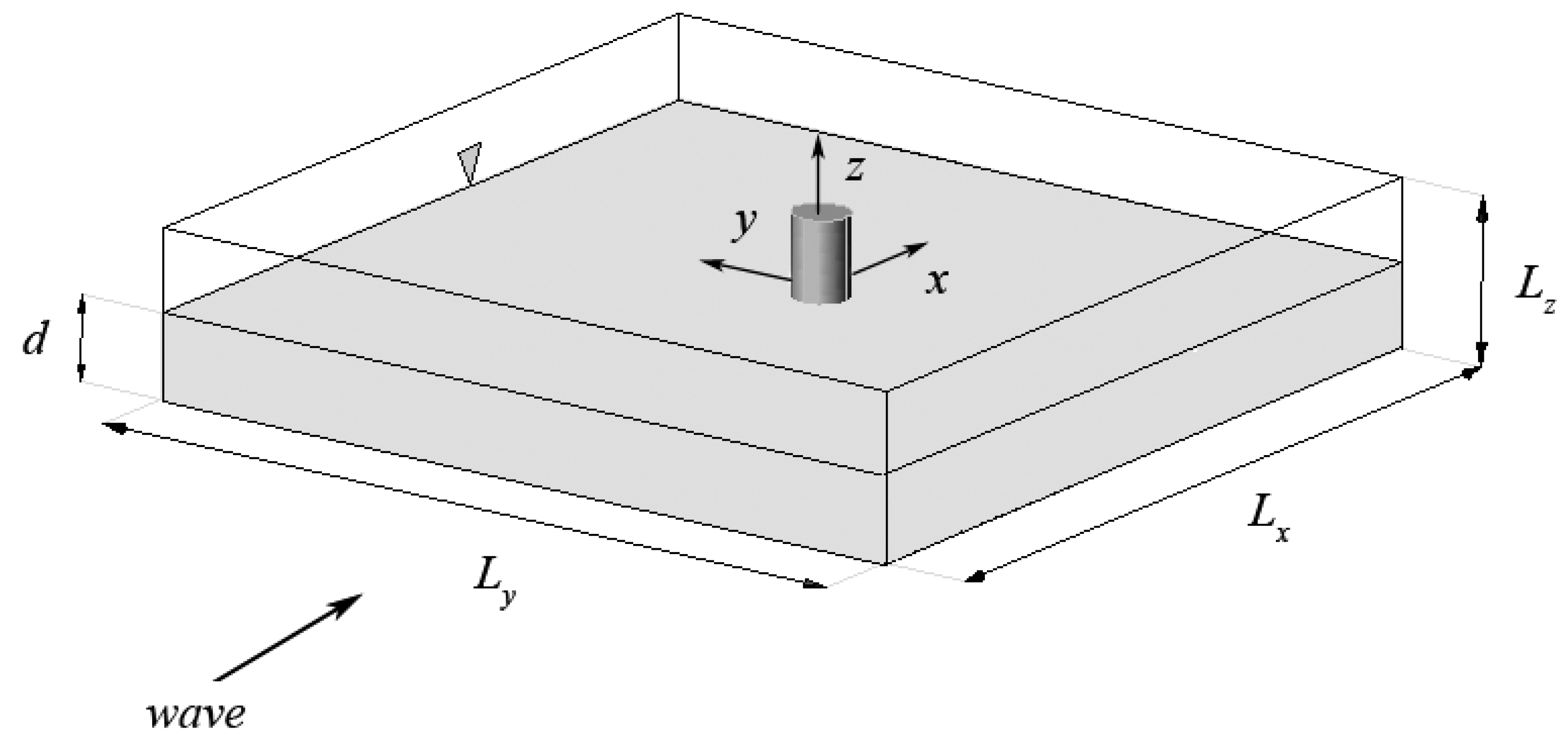
3.3. Numerical Integration of the Navier-Stokes Equations

The system of the three-dimensional, non-dimensional, time-dependent full Navier-Stokes equations in primitive variables (body forces are included) is considered (the fluid is incompressible and viscous, Einstein summation convention applies to repeated indexes, i, j = 1, 2, 3):
u i t + u j u i x j = p x i + 1 Re N S 2 u i x j x j + δ i , 3
u i x i = 0
Variables and operators have been here nondimensionalized by the cylinder diameter ( D ) for lengths, by the group ( D g ) for velocities, by ( ρ D g ) for pressures, by ( D / g ) for time, where Re N S is the Reynolds number resulting from the above nondimensionalization procedures.
The Reynolds number Re N S and the wave-field Reynolds number defined in Equation (7) are related as follows:
Re N S = D g D / ν = 2 π Re / K C D L tanh ( k d )
For the execution of the calculations, the Flow-3D computational code [30] has been further used, that solves the fluid governing equations using the finite-volume technique. In this code the free-surface condition is handled with the VOF method [29], and the Fractional Area Volume Obstacle Representation (FAVOR) technique is used for the modeling of complex geometries.
According to the VOF method, the portion of the volume occupied by the obstacle in each computational cell is defined at the beginning of the work. The fluid fraction in each cell is calculated, and the equations for the fluid-fraction volumes are formulated using the FAVOR function. The finite-volume technique—on staggered cuboid computational cells—is used for the discretization of the governing equations. The meshing technique does not induce any mesh distortion during transients, and a multi-block meshing technique is available, to provide higher resolutions in the calculations, where needed. With respect to time, most terms in the equations are evaluated explicitly, exception made for the pressures. Pressures and velocities are coupled implicitly using time-advanced pressures in the momentum equation and time-advanced velocities in the mass-conservation equation. The coupled sets of equations resulting from this semi-implicit formulation are solved iteratively. For the present Navier-Stokes wave-flow calculations, a modified Alternating Direction Implicit (ADI) scheme has been used [30].
Boundary conditions of no-slip (and zero wall-normal velocity) at the cylinder external walls have been imposed. On the two x-z lateral boundary planes of the computing domain (Figure 3), symmetry conditions have been set, on the y-z end-plane outflow conditions have been enforced, while the free-surface condition holds at the wave surface. At the y-z inlet plane, the flow field corresponding to the incident wave of the case at hand is generated.
For the present Navier-Stokes wave-flow calculations (and also for the other simulations), a specially-assembled computing system has been used, that includes 2 Intel Xeon 5660 exa-core multi-core processors (a total of 12 CPUs available), a maximum of 48 GB of RAM, and up to 1.8 TB of mass memory (see also Alfonsi et al. [31,32,33]).
Recall that, by applying the curl operator to the Navier-Stokes equations, after some manipulations, one obtains the system of the vorticity-transport equations:
ω i t + u j ω i x j = ω j u i x j + ν 2 ω i x j x j
ω i x i = 0
Now, the first term on the rhs of Equation (24) represents the rate-of-deformation of the vortex lines, while the second term on the rhs of Equation (24) represents the vorticity rate-of-diffusion, due to fluid viscosity. Equations (24) and (25) are of utmost importance to fluid mechanics and wave phenomena in particular, in that they mirror, in terms of vorticity field, the effects of the viscous forces. An unbalanced shear stress can exist only when the vorticity is nonzero, so that the existence of vorticity means that a particle is (or in its past history has been) subjected to net viscous forces. As for the representation of the results arising from numerical simulations, the vorticity field has been often used as a tool to gain new insights on flow phenomena, and in particular in the case of the flow around a circular cylinder (among others, Alfonsi [34,35,36], Alfonsi and Giorgini [37,38]). Though, the need of a deep understanding of many complex flow phenomena has soon motivated the consideration of the vorticity field as associated to the flow vortical structures (Alfonsi [39,40]), in a distinction with respect to the background, noncoherent vorticity field (see at Section 4.1).

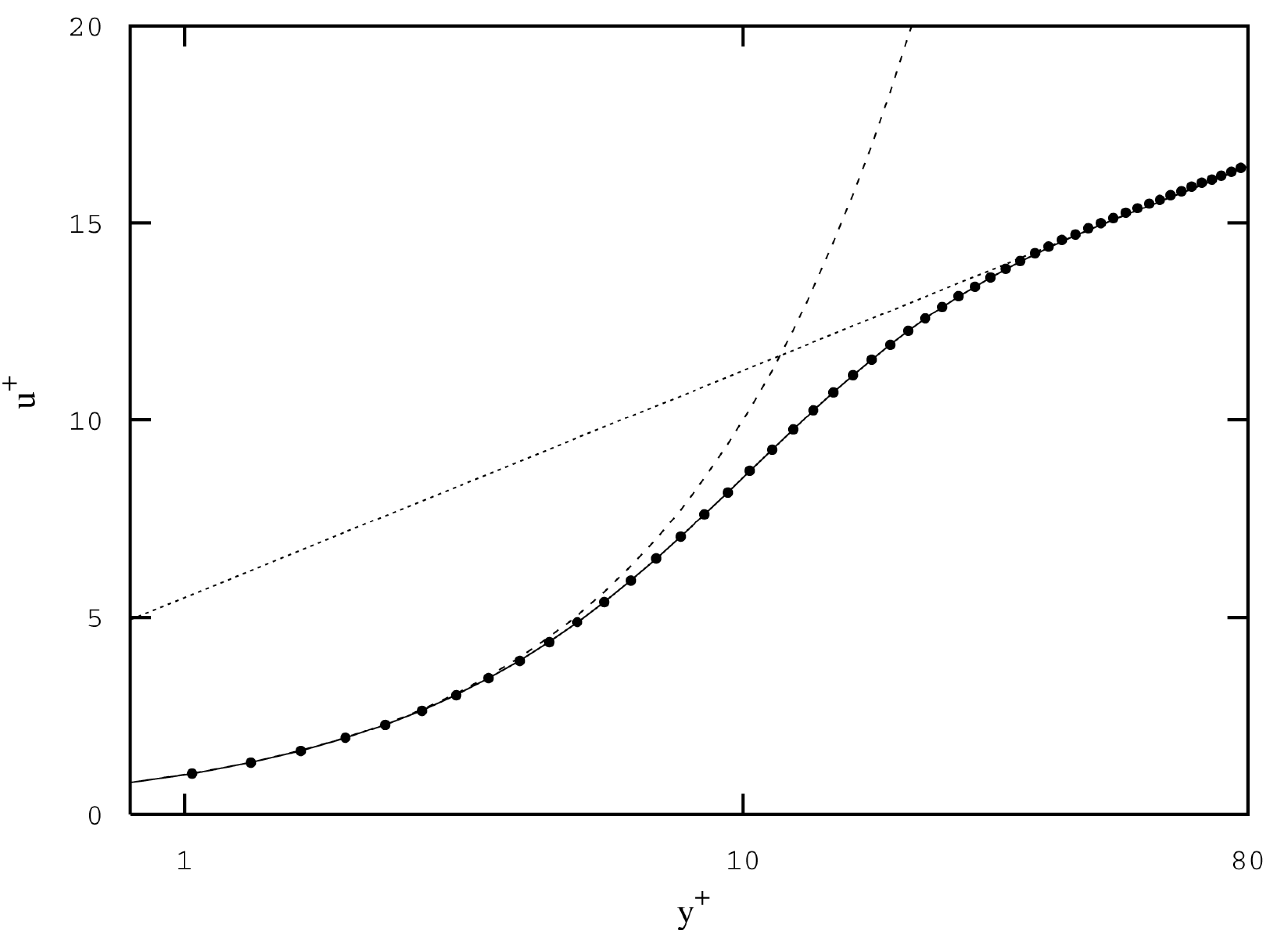
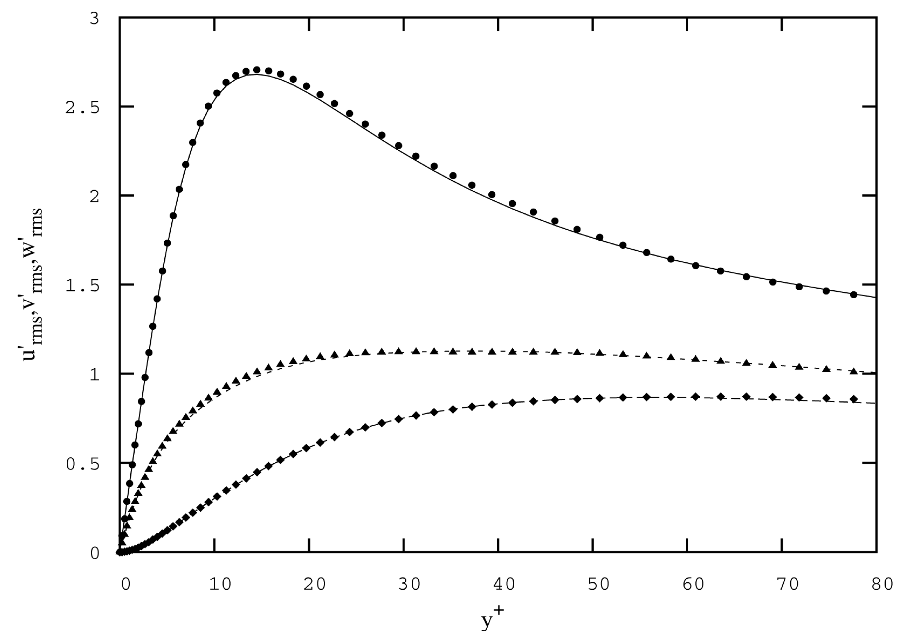
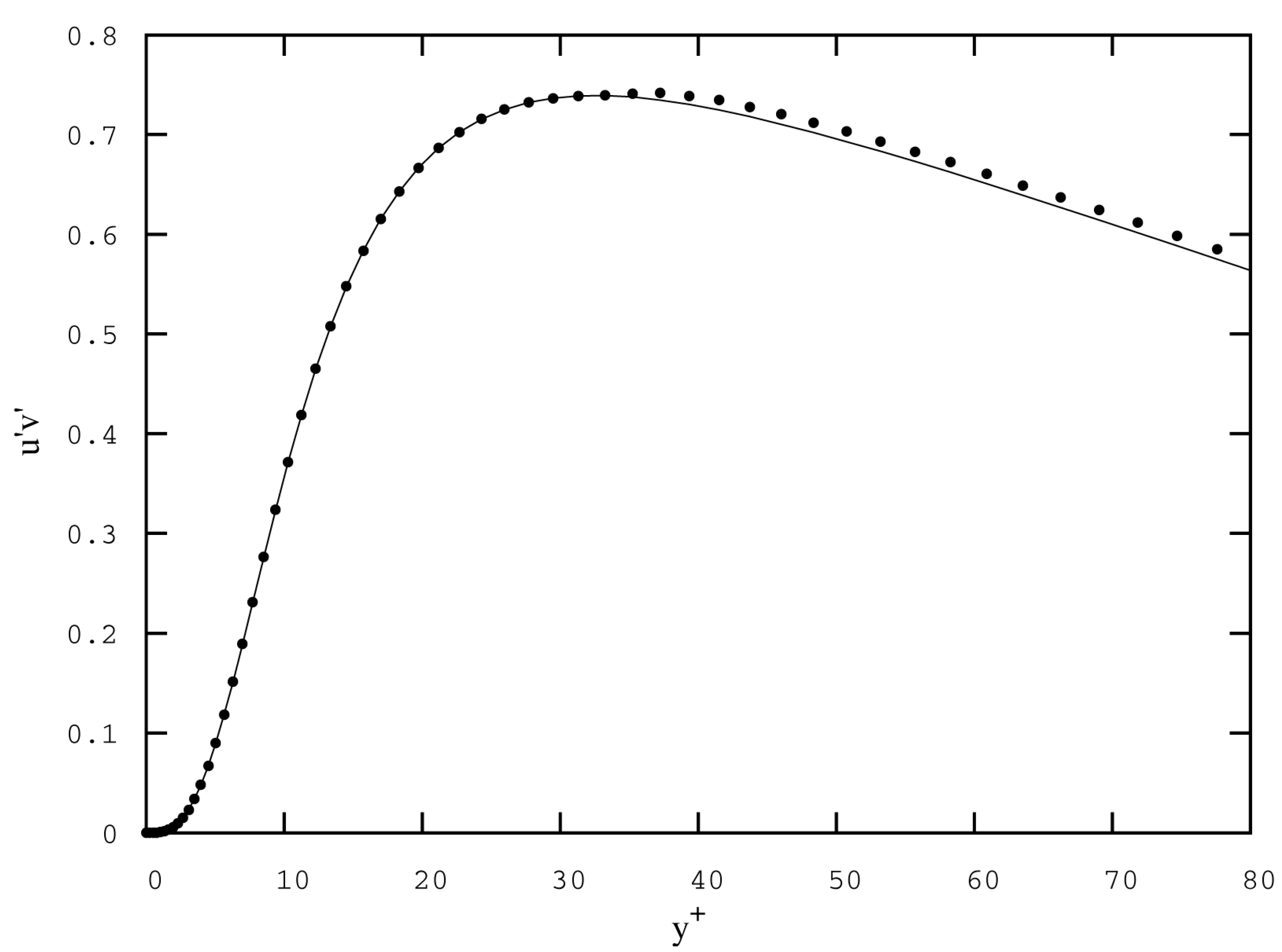
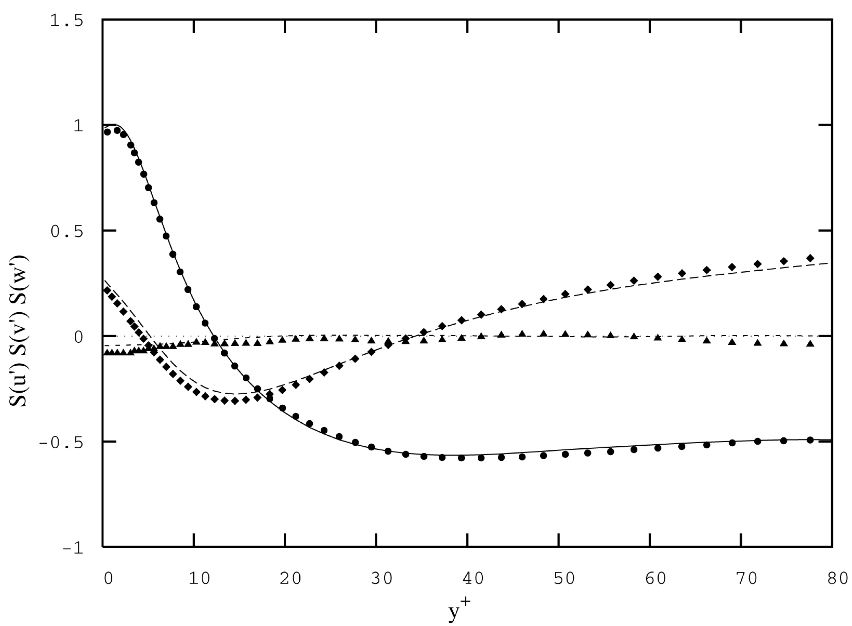
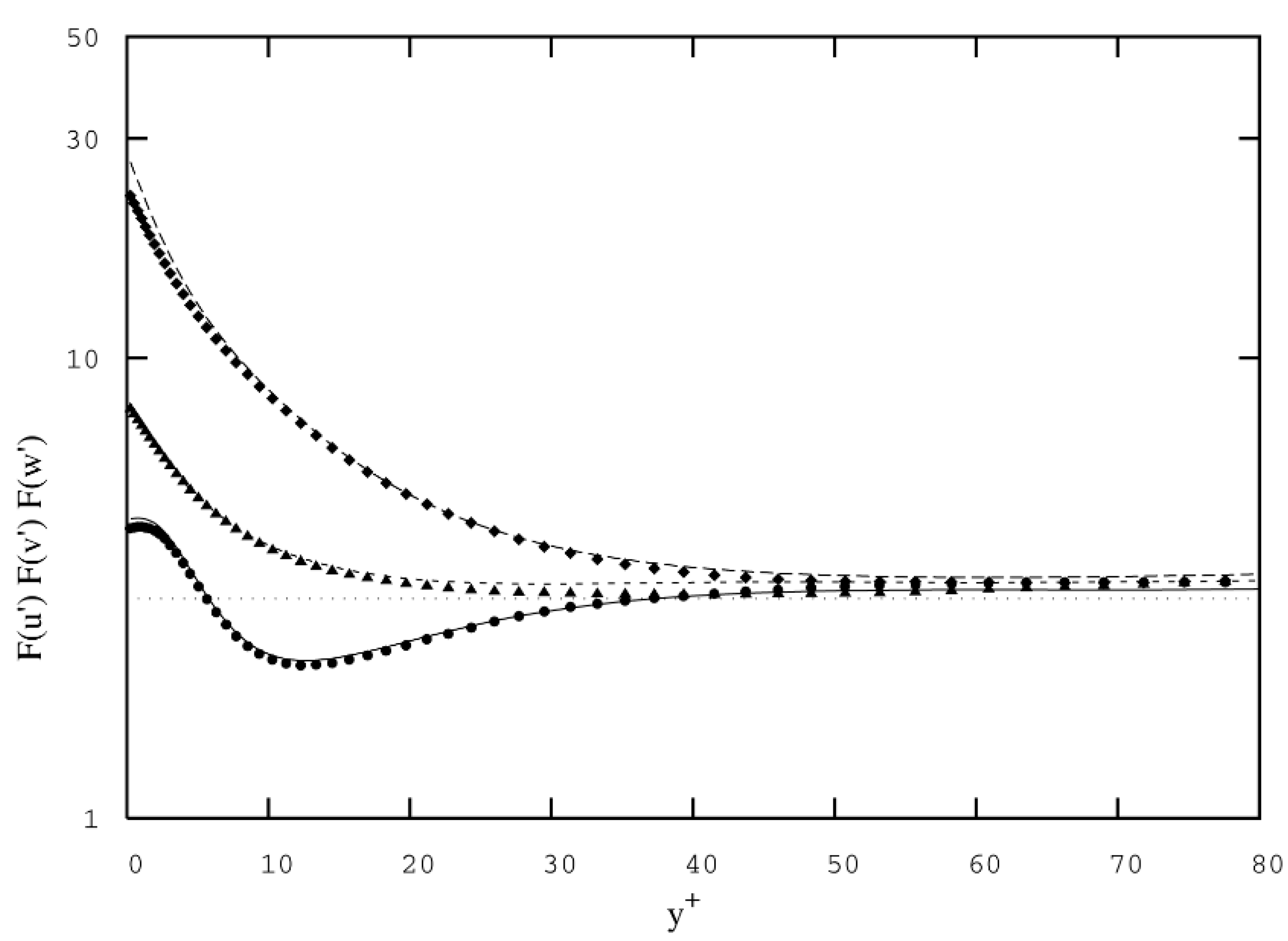
3.3.1. Validation of the Navier-Stokes Solver

Before actually running the present-work numerical simulations, an extensive work has been performed in order to appropriately validate the Flow-3D Navier-Stokes solver. Flow-3D is a widely-known computational code, and in the recent past several authors have performed scientific works directed to its validation. Among others, Kocaman et al. [41], Cho [42], Jin and Meng [43], Kim et al. [44], and Kayser and Gabr [45] have validated the Flow-3D solver in steady and unsteady problems involving cylinders and free surfaces, always obtaining rather satisfactory results. Though, in the present context, the issue of validation is in some way subtle. In performing the present numerical simulations by using the DNS approach, for the evaluation of the quality of the results, it becomes essential that the fluctuating portions of the velocity fields are correctly caught by the calculations. Thus, for validation, a rather demanding problem under this aspect has been chosen, namely the flow of a viscous fluid in a plane channel (recall that all the wave cases considered in present work fall in the no-separation, shear-flow Zone A of Figure 2). The plane-channel-flow case has a long tradition in the field of the numerical integration of the Navier-Stokes equations with the DNS technique, so becoming a true reference case. In spite of its apparently-simple geometry, it probably represents the most complex shear-flow case one can find, with regard to the possibility for the flow of developing a full cascade of scales, that only depend on the value of the Reynolds number that one is able to reach (see [23] and references therein). Then, the Flow-3D Navier-Stokes code has been validated in the plane-channel flow case against a reference, rather accurate code, namely the mixed spectral-finite difference Navier-Stokes solver originally developed by Alfonsi et al. [46] and further tested by Passoni et al. [47,48,49]. This latter solver has extensively proven to be able to accurately calculate several quantities that characterize shear flows (Alfonsi and Primavera [50]). In the framework of the validation procedure, high-order statistical moments of the fluctuating portions of the velocity fields have been computed, so that, according to the fact that the validation process has given rather satisfactory results, one is now confident that the flow scales, the flow structures, and the most energetic flow modes that have been calculated in the present work, are correct.
Results and comparisons are now reported for the computational test-case simulations (see also at Table 3). In Figure 4 the mean-velocity profile (in wall coordinates), as calculated with the Flow-3D solver, is compared with the law of the wall and with the results given by the reference solver. Figure 4 shows that the viscous sublayer is well resolved, yielding the linear velocity distribution for y + < 5 . At larger distances from the wall ( y + > 30 ) the logarithmic velocity distribution with von Kármán constant κ = 0.4 , and additive constant C = 5.5 , is satisfactorily followed.
Figure 4. Computational test-case. Mean streamwise-velocity profile: (—) reference solver, (●●) Flow-3D solver, (―) law of the wall u + = y + , u + = 2.5 ln y + + 5.5 .
Computation 03 00386 g004
Table 3. Characteristic parameters used for the test-case simulations ( Re τ = 200 ).
Domain Dimensions ( 1 < y / h < + 1 , 200 < y + < + 200 )
L x L y L z L x + L y + L z +
4 π h 2 h 2 π h 25124001256
Computational Grid for the Reference Navier-Stokes Solver
N x N y N z N t o t
256181256 11.862 × 10 6
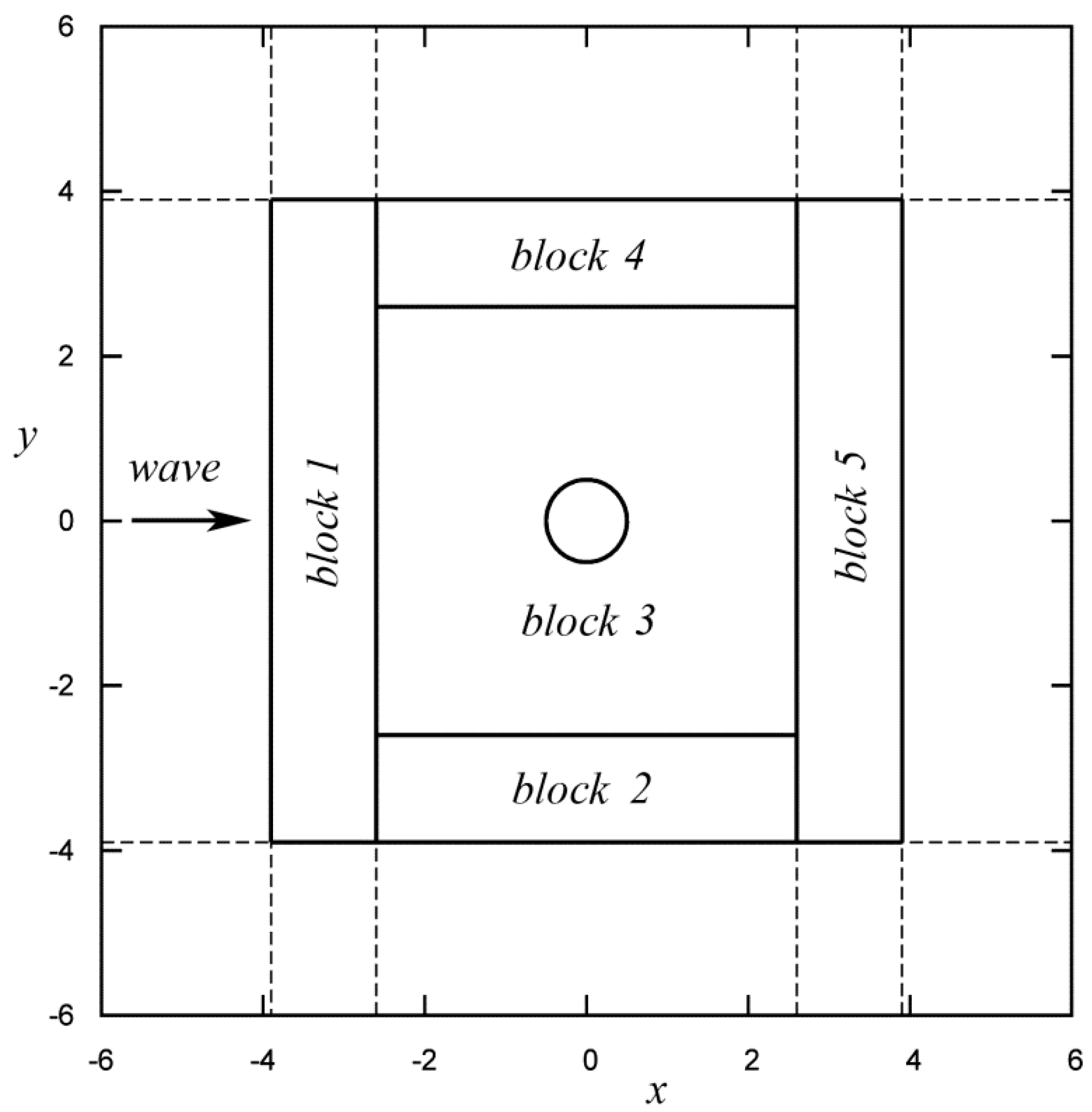
Multi-Bolck Computational Grid for the Flow-3D Navier-Stokes Solver
Block-subdivision along y N x N y N z N t o t
200 < y + < 198.54 304051520 23.1 × 10 6
198.54 < y + < 191.88 152013760≈ 15.1 × 10 6
191.88 < y + < 167.72 76018380≈ 5.2 × 10 6
167.72 < y + < + 167.72 380107190≈ 7.7 × 10 6
+ 167.72 < y + < + 191.88 76018380≈ 5.2 × 10 6
+ 191.88 < y + < + 198.54 152013760≈ 15.1 × 10 6
+ 198.54 < y + < + 200 304051520≈ 23.1 × 10 6
200 < y + < + 200 110201795510≈ 94.4 × 10 6
Figure 5 reports the rms values of the velocity fluctuations ( u r m s ) ,   ( v r m s ) ,   ( w r m s ) in wall coordinates. According to the Flow-3D solver, the position of the maximum value of the streamwise fluctuations results at y + = 14.51 , with a peak value of 2.70 (see also Mochizuki and Nieuwstadt [51], and Alfonsi [52]). Figure 6 reports the values of the Reynolds shear stress ( u v ¯ ) in wall coordinates, Figure 7 reports the skewness factors ( S u ) ,   ( S v ) ,   ( S w ) of the velocity fluctuations (in wall coordinates, while Figure 8 reports the flatness factors ( F u ) ,   ( F v ) ,   ( F w ) .
Figure 5. Computational test-case. Rms values of the velocity fluctuations; u r m s : (—) reference solver, (●●) Flow-3D solver; v r m s : (— — ) reference solver, (♦♦) Flow-3D solver; w r m s : (– – ) reference solver, (▲▲) Flow-3D solver.
Computation 03 00386 g005
Figure 6. Computational test-case. Reynolds shear stress; u v ¯ : (—) reference solver, (●●) Flow-3D solver.
Computation 03 00386 g006
Figure 7. Computational test-case. Skewness factors of the velocity fluctuations; S u : (—) reference solver, (●●) Flow-3D solver; S v : (— — ) reference solver, (♦♦) Flow-3D solver; S w : (– – ) reference solver, (▲▲) Flow-3D solver.
Computation 03 00386 g007
Figure 8. Computational test-case. Flatness factors of the velocity fluctuations; F u : (—) reference solver, (●●) Flow-3D solver; F v : (— —) reference solver, (♦♦) Flow-3D solver; F w : (– –) reference solver, (▲▲) Flow-3D solver.
Computation 03 00386 g008
According to the Flow-3D solver, the value of ( S u ) at the position ( y + | p e a k ) of the ( u r m s ) peak value, is 0.1419 , rather close to zero (see also Mochizuki and Nieuwstadt [51], Alfonsi [52]), while the flatness factor ( F v ) assumes a value of about 24 approaching the walls, so denoting the highly intermittent character of the normal velocity fluctuation near the solid border (see also Xu et al. [53], Alfonsi [54], Alfonsi et al. [55,56]). Overall, the comparisons between the results given by the Flow-3D Navier-Stokes solver and those given by the reference solver, are rather satisfactory.

3.3.2. Accuracy of Calculations and Computing Procedures

In the Navier-Stokes simulations of present work, no models for the fluctuating portion of the velocity field have been used, so that the viscous-flow governing equations are solved following the DNS approach. Direct Numerical Simulation consists in solving numerically the full Navier-Stokes equations with physically-consistent accuracy in space and time, in such a way as to resolve all the essential flow scales. If the mesh is fine enough, and the numerical scheme is designed to minimize the dispersion and dissipation errors, one obtains an accurate three-dimensional, time-dependent solution of the equations at hand. As concerns the smallest-scale-resolution requirements in DNS calculations, the criterion is usually followed of resolving the Kolmogorov space and time microscales:
η = ( ν 3 ε ¯ ) 1 / 4 ;   τ η = ( ν ε ¯ ) 1 / 2
or, at most, limited multiples of the latter.
As concerns the procedure for the evaluation of the Kolmogorov scales as defined in Equation (26), they can be evaluated by estimating the average rate of dissipation of kinetic energy per unit mass ( ε ¯ ), as obtained from some mean-flow quantities (Bakewell and Lumley [57]). In the case of present work, one obtains:
ε ¯ 2 π r 0 d τ w u max ρ ( L x L y d π r 0 2 d ) = F f u max ρ d ( L x L y π r 0 2 )
where ( F f ) is the portion-due-to-friction of the total in-line force exerted on the cylinder.
Recall that, for small values of the Keulegan-Karpenter number and intermediate values of the Reynolds number, it is possible to determine the in-line forces on the basis of the asymptotic theory of Bearman et al. [58] (see also Morison et al. [59]). On this basis, the latter quantity (per unit length) is given by:
F f = 1 2 ( 1 + i ) ρ ω D 2 u max ( π β ) 1 / 2 e i ω t
so that, for the wave-case of present work (see also at Table 4), one obtains:
ε ¯   0.00000525   D 1 / 2 g 3 / 2 ;   η = 0.0147   D ;   τ η = 3.45   D / g
For the present Navier-Stokes wave-flow simulations, a linear wave case has been selected, with characteristic parameters included in the range of values reported in Table 1 (so belonging to Zone A of Figure 1). These parameters are extensively reported in Table 4, in conjunction with the related main computational parameters.
The computing domain (Figure 3) has been discretized into a 5-block, multiblock computational grid (Figure 9). The partitions of the computing domain occupied by each grid-point block and the grid-point distances ( Δ x , Δ y , Δ z ) within each block or group of blocks, are reported in Table 4.
Figure 9. Subdivision of computing domain in grid-point blocks (top view).
Computation 03 00386 g009
It is to be noted in particular that: (i) along the z-direction, Δ z assumes the same constant value through the different blocks; (ii) as concerns Δ x and Δ y along the x- and the y-directions, respectively, the grid point-distances are constant in the peripheral blocks 1, 2, 4, 5, while within the internal block 3, they are distributed non-uniformly according the hyperbolic-tangent grid-stretching law:
x s t r = r 0 + [ L 3 r 0 ] { 1 P P ( 1 x ) ( 1 P P ) [ 1 tanh ( Q Q x ) tanh ( Q Q ) ] }
y s t r = r 0 + [ L 3 r 0 ] { 1 P P ( 1 y ) ( 1 P P ) [ 1 tanh ( Q Q y ) tanh ( Q Q ) ] }
where P P = 1.7 and Q Q = 1.9 ( L 3 is the half length of block 3, both along x and y, see at Figure 9). With the aforementioned grid-point configuration, the space resolutions ( Δ x ) and ( Δ y ) at the cylinder wall are able to resolve less than one half of the Kolmogorov spatial microscale, while at the domain external boundaries they are still able to resolve less than two and a half η . These latter values are perfectly in the ranges usually adopted in DNS ([23]).
Table 4. Characteristic parameters used for the Navier-Stokes wave-flow.
Field Parameters ( K C = 0.578 , Re = 1862 , β = Re / K C = 3221 )
DLHad r 0
[D units][D units][D units][D units][D units][D units]
13.9060.1830.091520.50
η T τ η u max D / L H / r 0
[D units][ D / g units][ D / g units][ D g units]
0.01474.9623.4500.1160.2560.367
H / L ( H / L ) M a x 1 ( H / L ) M a x 2 d / L kd k r 0
0.0470.1390.06960.5123.2170.809
Computational Parameters [D Units]
L x ( = 2 L ) L y ( = 2 L ) L z ( = 3 d ) L 1 = L 2 = L 4 = L 5 L 3
7.87.83.01.32.1
block 1 3.9 < x < 2.6 3.9 < y < 3.9 2 < z < 1.0 N b l o c k _ 1 = 1,156,200
block 2 2.6 < x < 2.6 3.9 < y < 2.6 2 < z < 1.0 N b l o c k _ 2 = 702,240
block 3 2.6 < x < 2.6 2.6 < y < 2.6 2 < z < 1.0 N b l o c k _ 3 = 14,953,080
block 4 2.6 < x < 2.6 2.6 < y < 3.9 2 < z < 1.0 N b l o c k _ 4 = 702,240
block 5 2.6 < x < 3.9 3.9 < y < 3.9 2 < z < 1.0 N b l o c k _ 5 = 1,156,200
blocks 1-5 3.9 < x < 3.9 3.9 < y < 3.9 2 < z < 1.0 N t o t = 18,669,960
Space and Time Resolutions [ η and τ η Units]
Δ x c y l i n d e r _ w a l l = 0.45 η Δ x e n d _ o f _ b l o c k _ 3 = 2.25 η Δ x b l o c k s _ 1 , 5 = 2.25 η
Δ z b l o c k s _ 1 , 2 , 3 , 4 , 5 = 1.70 η Δ t = 0.002 τ η

4. Flow-Field Analysis

4.1. Overview of Swirling-Strength Criterion for Flow-Structure Extraction

Of the existing techniques for the extraction of flow vortical structures (Alfonsi [39,40], Alfonsi and Primavera [60,61]) in the present work the criterion of the imaginary part of complex eigenvalue pair of the velocity-gradient tensor (the swirling-strength or also the λ c i criterion) as devised by Zhou et. al. [62], has been adopted.
By considering the system of the flow governing equations, an arbitrary point O can be chosen in the field, and a Taylor-series expansion of each velocity component can be performed in terms of space coordinates with the origin in O, so that the first-order pointwise linear approximation at that point becomes:
u i = A i + A i j x j
where A i j = u i / x j is the velocity-gradient tensor. If O is located at a critical point, the zero-order terms of (22) are zero, and from the characteristic equation of A i j , one has:
λ 3 + P λ 2 + Q λ + R = 0
where:
P = t r ( A i j )
Q = 1 2 { [ t r ( A i j ) ] 2 t r ( A i j 2 ) }
R = det ( A i j )
are the scalar invariants of the velocity-gradient tensor (tr is trace, det is determinant). In the case of incompressible flow, P = 0 , so that Equation (32), the second invariant ( Q ) of Equation (33b), and the discriminant ( D s c ) of the characteristic equation of A i j , become respectively:
λ 3 + Q λ + R = 0
Q = 1 2 t r ( A i j 2 )
D s c = R 2 4 + Q 3 27
when ( D s c > 0 ), the velocity-gradient tensor has one real eigenvalue ( λ 1 ) and a pair of complex-conjugate eigenvalues ( λ 2 , λ 3 ). Zhou et al. [62] adopted the criterion of identifying vortices by visualizing isosurfaces of prescribed values of the imaginary part of the complex-eigenvalue pair of the velocity-gradient tensor. In particular, one has:
λ 1 = λ r ;   λ 2 = λ c r + i λ c i ;   λ 3 = λ c r i λ c i
The swirling strength ( λ c i ) represents a measure of the local swirling rate inside a vortical structure, so that isosurfaces of the imaginary part of the complex eigenvalue pair of the velocity-gradient tensor can be used to visualize vortices. The method is frame independent and, due to the fact that the eigenvalue pair is complex only in regions of local circular or spiralling streamlines, it automatically eliminates regions having no local spiralling motion. The method has proven to give rather satisfactory results in several different flow cases (Alfonsi [63], Alfonsi and Primavera [64,65], Alfonsi et al. [66,67,68,69,70]).

4.2. Overview of Karhunen-Loève Decomposition Technique

Within the group of the Proper Orthogonal Decomposition (POD) methods (see Liang et al. [71], Alfonsi [39,40]) a powerful technique for the extraction of the most energetic modes of a flow is the Karhunen-Loèwe (KL) decomposition (see also Lumley [72], Sirovich [73]).
By considering an ensemble of temporal realizations of a non-homogeneous, square integrable (with finite kinetic energy), three-dimensional velocity field u i ( x j , t ) with ( i , j = 1 , 2 , 3 ) , on a finite domain Λ , one wants to find the most similar function to the elements of the ensemble on average (operator ), i.e., to determine the highest mean-square correlated structure with all the elements of the ensemble. This corresponds to find a deterministic vector function φ i ( x j ) that maximizes the normalized inner product of the candidate structure with the field. A necessary condition for this problem is that the above-mentioned function φ i ( x j ) is an eigenfunction, solution of the eigenvalue problem and first-kind Fredholm integral equation:
Λ R i j ( x l , x l ) ϕ j ( x l ) d x l = Λ u i ( x k , t ) u j ( x k , t ) ϕ j ( x k ) d x k = λ ϕ i ( x k )
where i , j , l , k = 1 , 2 , 3 .
In Equation (36), R i j = u i ( x l , t ) u j ( x k , t ) is the two-point velocity-correlation tensor, and the maximum value of φ i ( x j ) corresponds to the largest eigenvalue λ of R i j . When Λ is bounded, based on the Hilbert-Schmidt theory, there exists a denumerable infinity of solutions of Equation (36), where these solutions are called the empirical eigenfunctions [ φ i ( n ) ( x j ) , normalized, i.e., φ i ( n ) ( x j ) =1]. The orthonormality of the empirical eigenfunctions implies that structures of different order do not interact which each other in their contribution to second order statistics. To each empirical eigenfunction is associated a real and positive eigenvalue λ ( n ) ( R i j is non-negative by construction), and the eigenfunctions form a complete set. Thus, every member of the originary ensemble can be reconstructed by means of a modal decomposition in the eigenfunctions themselves:
u i ( x j , t ) = n a n ( t ) φ i ( n ) ( x j )
that can be seen as a decomposition of the originary random field into deterministic structures φ i ( n ) ( x j ) , with random, time-dependent, coefficients. The modal amplitudes (the time series of the coefficients a n ( t ) when related to velocity fields varying with time) are uncorrelated, and their mean- square values are the eigenvalues themselves:
a n ( t ) a m ( t ) = δ n m λ ( n )
where δ n m is the Kroneker’s delta. A diagonal decomposition of the two-point velocity-correlation tensor holds:
R i j ( x l , x k ) = n λ ( n ) φ i ( n ) ( x l ) φ j ( n ) ( x k )
implying that the contribution of each different structure to the kinetic energy of the flow can be separately calculated, as:
E = Λ u i ( x j , t ) u i ( x j , t ) d x j = n λ ( n )
where E is the total kinetic energy in the domain. Thus, each eigenvalue represents the contribution of each correspondent structure φ ( n ) to the total amount of kinetic energy.
The KL technique is optimal for modeling or reconstructing a signal in the sense that, for a given number of modes, the projection into the subspace used for modeling contains the most kinetic energy possible on average, or, equivalently, the decay of the tail of the empirical eigenspectrum is always faster (or at most as fast) than the tail of the spectrum based on any other possible basis, Fourier spectrum included. This technique has proven to give rather satisfactory results in several different cases (Alfonsi and Primavera [74,75,76,77], Alfonsi et al. [78,79,80], Carbone et al. [81], Vecchio et al. [82], and Zhang et al. [83]).
In the context of the problem here at hand, the high-performance computational code for the execution of KL calculations has been used, as originally developed by Alfonsi and Primavera [84,85]. The above-mentioned code is general, it can be used in all kind of problems, and operates directly in physical space. More in particular, the two-point velocity-correlation tensor in Equation (36) is calculated in its complete form, so that the optimal representation of the velocity field outlined above, is evaluated in all the three directions (x,y,z). Within the computational procedure, Equation (36) is evaluated numerically by using the weight functions of the trapezoidal rule, and a scaling transformation is used to recover the symmetry in the resulting eigenvalue problem, that originally is not symmetric due to the fact that a non-uniformly spaced grid of point locations characterizes the three-dimensional computational domain involved in the decomposition operations.
For the execution of the KL decomposition (only Navier-Stokes fields are involved), the following procedure has been followed. Mainly due to limits in the computational resources available, a spatial subdomain has been selected within the whole computing domain in which the Navier-Stokes calculations have been executed. The subdomain involves ( N x = 49 , N y = 80 , N z = 10 , N t o t = 39 , 200 ) grid points, and is located immediately upstream from the cylindrical body (see at subsequent Figures).
With respect to time, the flow-field instants considered for the analysis are listed in Table 5. As a result of the decomposition procedure, a total of N x × N y × N z × 3 = 117 , 600 three-dimensional eigenfunctions (and corresponding eigenvalues) have been calculated in the subdomain. In Table 6, the individual fractions of energy as in Equation (40), and the cumulative energies are listed for the first ten KL modes. From the data reported in Table 6, it can be noted that the first three eigenfunctions exhibit alone a cumulative energy content of more than 99.8% of the total kinetic energy of the original velocity field.
Table 5. Flow-field instants involved in the KL decomposition (T is wave period).
Instant Number ( t )Instant ( D / g Units)Instant ( T Units)
10.0000.000
20.8760.144
32.4810.500
43.7220.750
54.9621.000
Table 6. Energy content of the first ten eigenfuctions of the KL decomposition.
Mode NumberEnergy FractionEnergy Sum
10.878180.87818
20.107700.98588
31.2271 × 10 2 0.99815
45.0327 × 10 3 1.00
52.6852 × 10 3 1.00
69.2960 × 10 4 1.00
75.5663 × 10 6 1.00
81.2803 × 10 6 1.00
93.5057 × 10 7 1.00
102.1537 × 10 7 1.00

5. Results

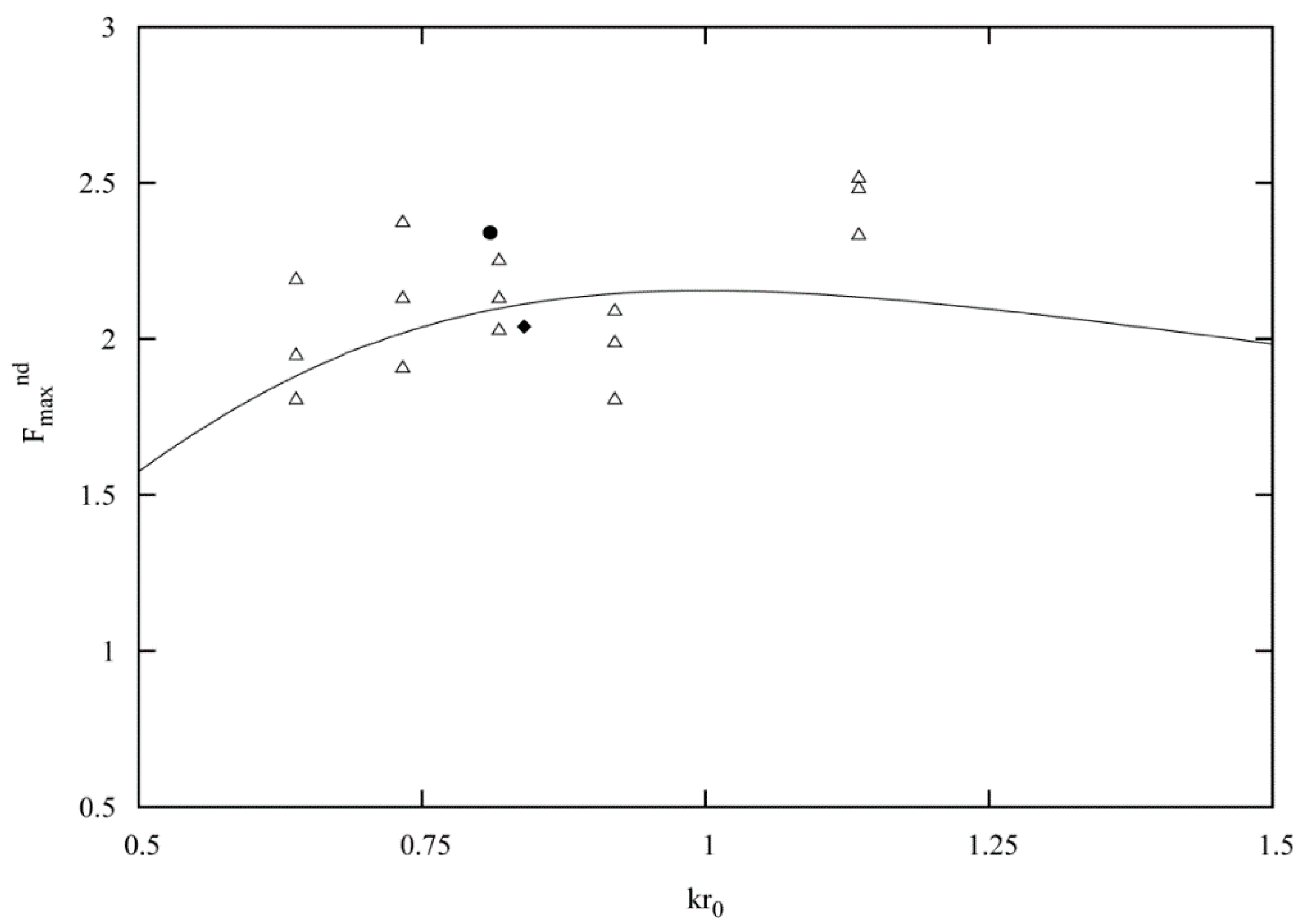
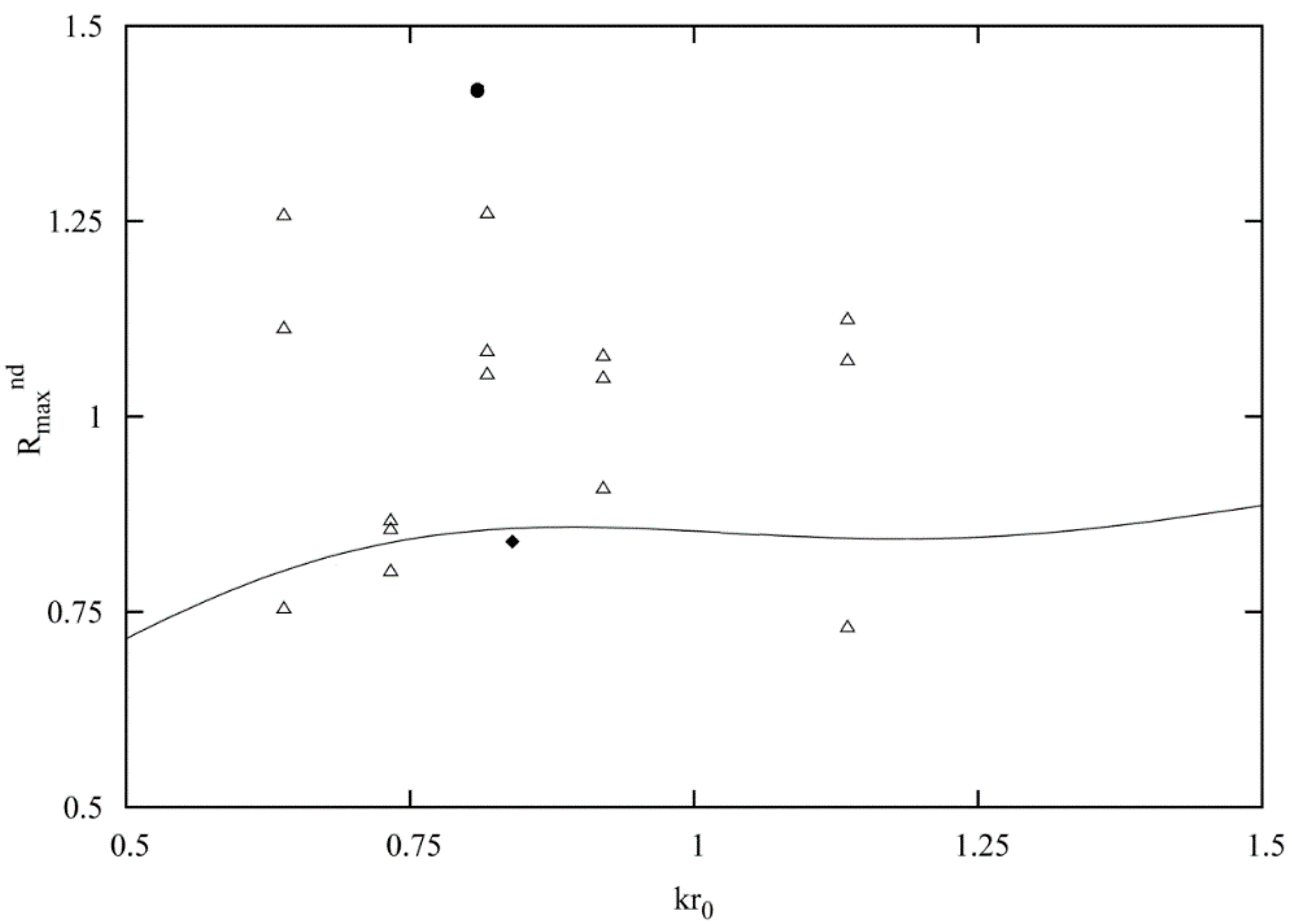
5.1. Forces and Runups

Figure 10 reports the values of the maximum nondimensional force on the cylinder ( F max n d ) obtained in the present Euler and Navier-Stokes simulations (the reported values are related to the first wave, once the condition of regular wave train is reached), in a comparison with linear theory and with the experimental data of [14]. From Figure 10 it can be noticed that linear theory slightly underestimates the wave force with respect to the results given by both our Navier-Stokes simulations and the experimental results [14]. Figure 11 reports the values of the maximum nondimensional runup on the cylinder ( R max n d ) obtained in the present Euler and Navier-Stokes simulations, again in a comparison with linear theory and with the experimental data of [14]. From Figure 11, it can be noted that the circumstance that linear theory strongly underestimates the real-fluid wave runup, is confirmed by the results of our Navier-Stokes simulations. This result is also valid for the experimental data obtained by Niedzwecki and Duggal [14] (exception made for a few of their values that fall under the potential-theory line). From Figure 10 and Figure 11 it can be also noted that, in both cases of forces- and runups results, the agreement between the values obtained from the numerical integration of the Euler equations and the potential-theory results is rather good, showing that when inviscid fluids are considered, both potential theory and primitive-variable mass- and momentum-conservation (Euler) equations, give, in practice, the same results. This circumstance demonstrates the fact that all the differences that one finds between inviscid-fluid- and viscous-fluid results, have to be attributed to the effects of the real-fluid, viscosity-generated shear-stress field.
Figure 10. Force ( F max n d ) on cylinder as a function of k r 0 : (—) solution of MacCamy and Fuchs [1]; (♦♦) data from solution of Euler equations; (●●) data from solution of Navier-Stokes equations; (∆∆) data from experiments of Niedzwecki and Duggal [14].
Computation 03 00386 g010
Figure 11. Runup ( R max n d ) on cylinder as a function of k r 0 : (—) solution of MacCamy and Fuchs [1]; (♦♦) data from solution of Euler equations; (●●) data from solution of Navier-Stokes equations; (∆∆) data from experiments of Niedzwecki and Duggal [14].
Computation 03 00386 g011

5.2. Velocity Potential

As a result of the computing procedures previously outlined at Section 3.1, results related to the φ derived flow fields are presented. In Figure 12 and Figure 13, the velocity-potential-derived flow fields are shown, in terms of free-surface elevation in the domain, at times t F max φ , and t R max φ , respectively.
Figure 12. Velocity-potential-derived free-surface profile. Top view of computing domain, at: (a) t = t F max φ ; (b) t = t R max φ .
Computation 03 00386 g012
Figure 13. Velocity-potential-derived free-surface profile. Side view of computing domain, at: (a) t = t F max φ ; (b) t = t R max φ .
Computation 03 00386 g013
The φ derived fields show first that—as already widely known—the wave exhibits the maximum runup on the cylinder at a later instant ( t R max φ ), with respect to that at which it exerts the maximum force on the obstacle ( t F max φ ).
Moreover, and as expected, the application of the swirling-strength criterion for structure extraction to the φ derived velocity fields, has given no results, due to the pure mathematical nature of the latter fields.

5.3. Euler Equations

As a result of the computing procedures previously outlined (Section 3.2), results related to the Euler-equations-derived flow fields are presented.
It is to be preliminarly noted that the following figures incorporate three types of information, namely: (i) they depict the flow fields in terms of flow structures as extracted with the swirling-strength (or also λ c i ) criterion [62], and represented at given threshold values ( λ c i | t h , see Alfonsi and Primavera [64]), at different instants; (ii) “lines” eventually detectable in the visualizations actually represent borders between structures; (iii) the external surfaces of the flow structures are colored with the spanwise component of the vorticity ( ω y ), so that the sign and the intensity of the local-particle rotation can be inferred from the visualizations (more intense ω y coloring denotes stretching of vortex lines, less intense ω y coloring denotes shrinking of vortex lines, reddish areas denote positive ω y , bluish areas denote negative ω y , greyish areas denote zero ω y ).
Figure 14a,b show top views of the computing domain at t = t F m a x E u l e r (the instant at which the Euler-derived wave field exerts the maximum force on the cylinder) and t = t R m a x E u l e r (the instant at which the Euler-derived wave field exhibits the maximum runup on the upstream external surface of the cylinder), respectively. The fields are rather regular and substantially symmetric. The flow field exhibits a number of tubular vortical structures concentrated at the free surface, where, from the distribution of these structures, one obtains the perception of the free-surface configuration in terms of wave crests, troughs, accumulation of fluid mass upstream from the cylinder, and progressive development of the wave-diffraction phenomenon (see groups of lines a to d in Figure 14). In particular, at t = t F m a x E u l e r there exist a remarkable accumulation of fluid mass—mainly irrotational—upstream from the cylinder, while at t = t R m a x E u l e r both positive and negative vorticity contaminates the latter mass of fluid.
Overall, the nature of the above-mentioned free-surface tubular structures is that of being largely irrotational, exception made for the previously-generated vorticity contained in some of them that propagates (conservatively) across the field, according to the progression of the wave-cylinder interaction process. From Figure 14 it can be also noticed that the areas characterized by positive and/or negative, previously-generated ω y , are well defined and confined, showing that no viscous diffusion of vorticity occurs, as expected (in the absence of viscosity, no vorticity diffusion occurs).
Figure 14. Flow structures as obtained from the solution of the primitive-variable Euler equations. Top view of free-surface profile: (a) t = t F max E u l e r ; (b) t = t R max E u l e r .
Computation 03 00386 g014
Figure 14 further shows that the wave crest- and trough-structures are substantially irrotational, while positive and/or negative vorticity is present in the ascending and/or descending portions of the wave, approximately at half-way between a crest and a trough. Moreover, it can be noted that, at t = t F m a x E u l e r , the flow structures encompassed in the group of lines a (located in a descending portion of the wave, upstream from a trough) are characterized by strong positive vorticity, the structures encompassed by the group of lines b (right after a trough) are characterized by less intense positive vorticity, those encompassed by the group of lines c (downstream from a crest) are characterized by strong negative vorticity far away from the cylinder, and by strong positive vorticity nearby the cylinder (caused by the pressure field in the proximity of the cylindrical body), while the structures encompassed by the group of lines d are characterized by remarkably-less intense negative vorticity.
In going from t = t F m a x E u l e r to t = t R m a x E u l e r one can also notice that the structures encompassed in the group of lines a exhibit an increase of their positive ω y -field, due to the turning and stretching of vortex lines, as caused by the progression of the wave-to-cylinder approaching process, while the structures encompassed by the group of lines b also increase their ω y field (of either sign), due to the turning and stretching of vortex lines nearby the cylinder. Moreover, the structures encompassed by the group of lines c increase their negative ω y -field, due to the turning of vortex lines right downstream from the cylinder, while those encompassed by the group of lines d are subjected to remarkable turning and stretching between the wave trough and wave crest, downstream from the cylinder.
In Figure 15, Figure 16 and Figure 17, upstream-, side-, and downstream-close-up views of the structure field are shown in the vicinity of the cylinder external wall, at t = t F m a x E u l e r and t = t R m a x E u l e r , respectively. These figures show that other types of structures develop underwater, all of them of inviscid type. Arrow 1 indicates a structure completely encompassing the cylindrical body, that persists in going from t = t F m a x E u l e r to t = t R m a x E u l e r . Upstream from the cylinder, a rather complex structure is visible (structure 2/3), that only slightly changes its shape in going from t = t F m a x E u l e r to t = t R m a x E u l e r (note that, in the subsequent Navier-Stokes-field representations, structures 2 and 3 will appear as distinct).
Additional structures are present. In Figure 15 and Figure 16, arrow 4 denotes an upstream structure that represents the underwater counterpart of the accumulation of fluid mass upstream from the cylinder, that verifies when the oncoming wave approaches the cylindrical body. In Figure 16 and Figure 17, arrow 5 denotes a downstream structure that represents the underwater remnant of the wave-cylinder interaction process. In Figure 15, Figure 16 and Figure 17, a right-side structure and a left-side structure are also visible, mirroring the way trough which the structure field propagates from upstream to downstream from the cylinder, in the absence of viscous forces.
Figure 15. Close-up at the cylinder surface of inviscid-flow structures as obtained from the solution of the Euler equations. Upstream view: (a) t = t F max E u l e r ; (b) t = t R max E u l e r .
Computation 03 00386 g015
Figure 16. Close-up at the cylinder surface of inviscid-flow structures as obtained from the solution of the Euler equations. Side view: (a) t = t F max E u l e r ; (b) t = t R max E u l e r .
Computation 03 00386 g016
Figure 17. Close-up at the cylinder surface of inviscid-flow structures as obtained from the solution of the Euler equations. Downstream view: (a) t = t F max E u l e r ; (b) t = t R max E u l e r .
Computation 03 00386 g017

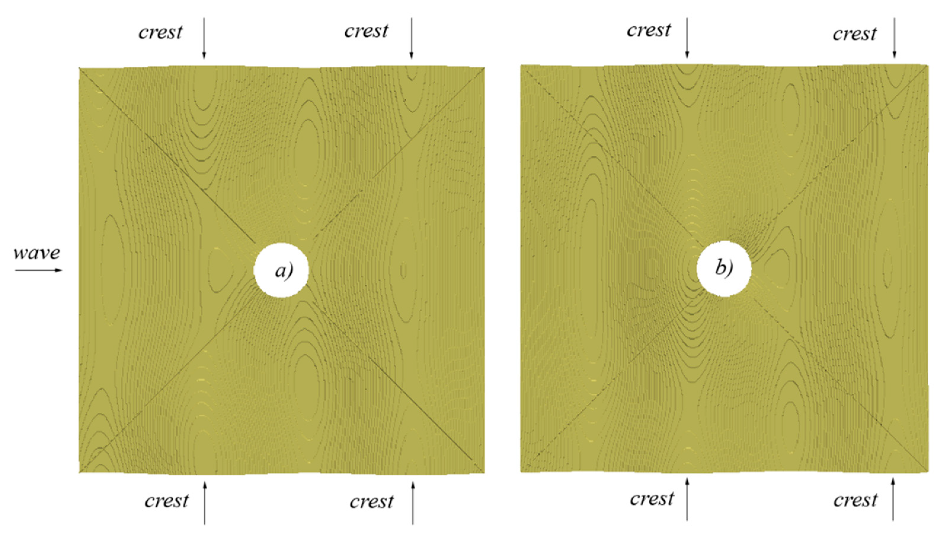
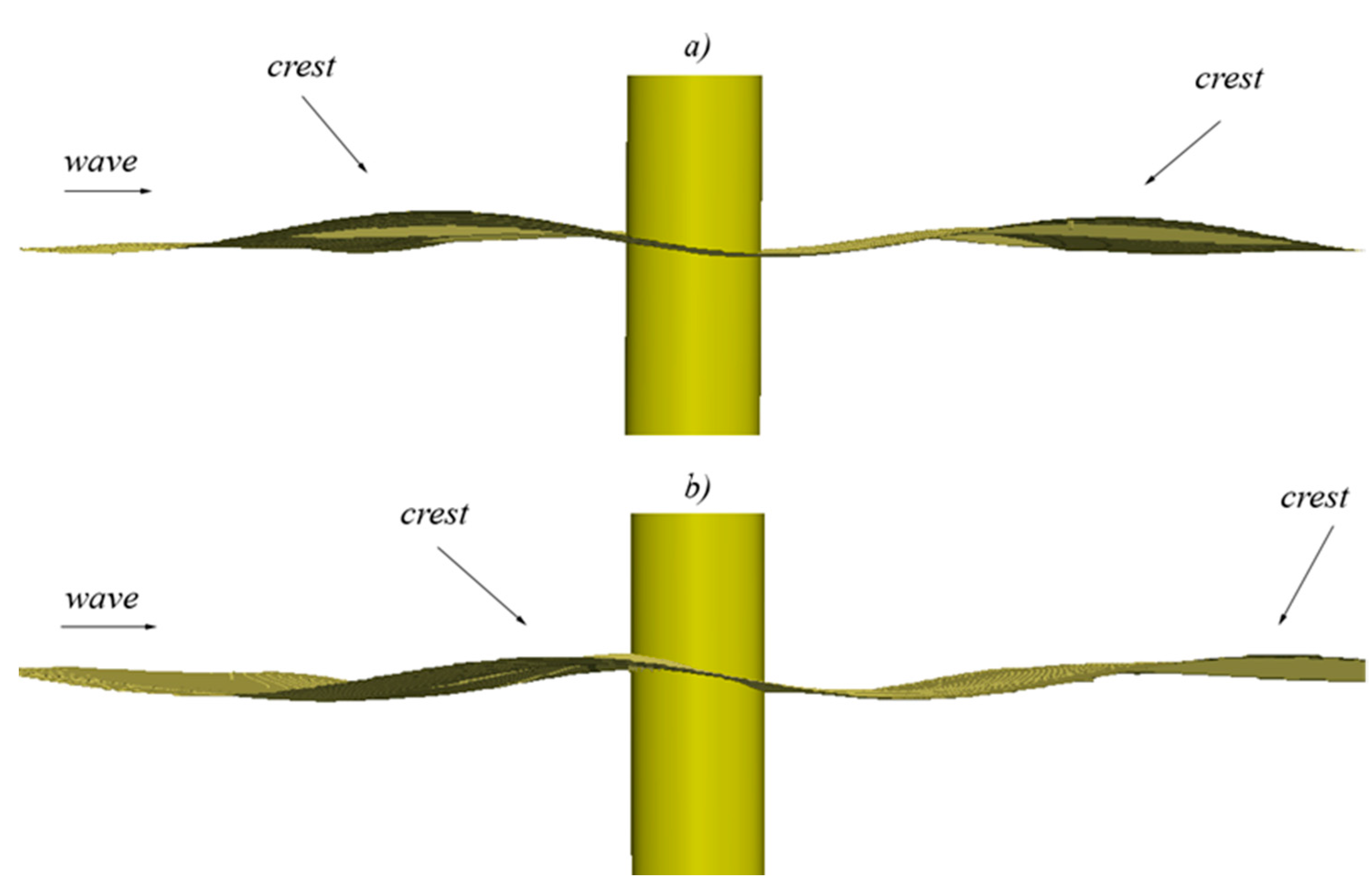
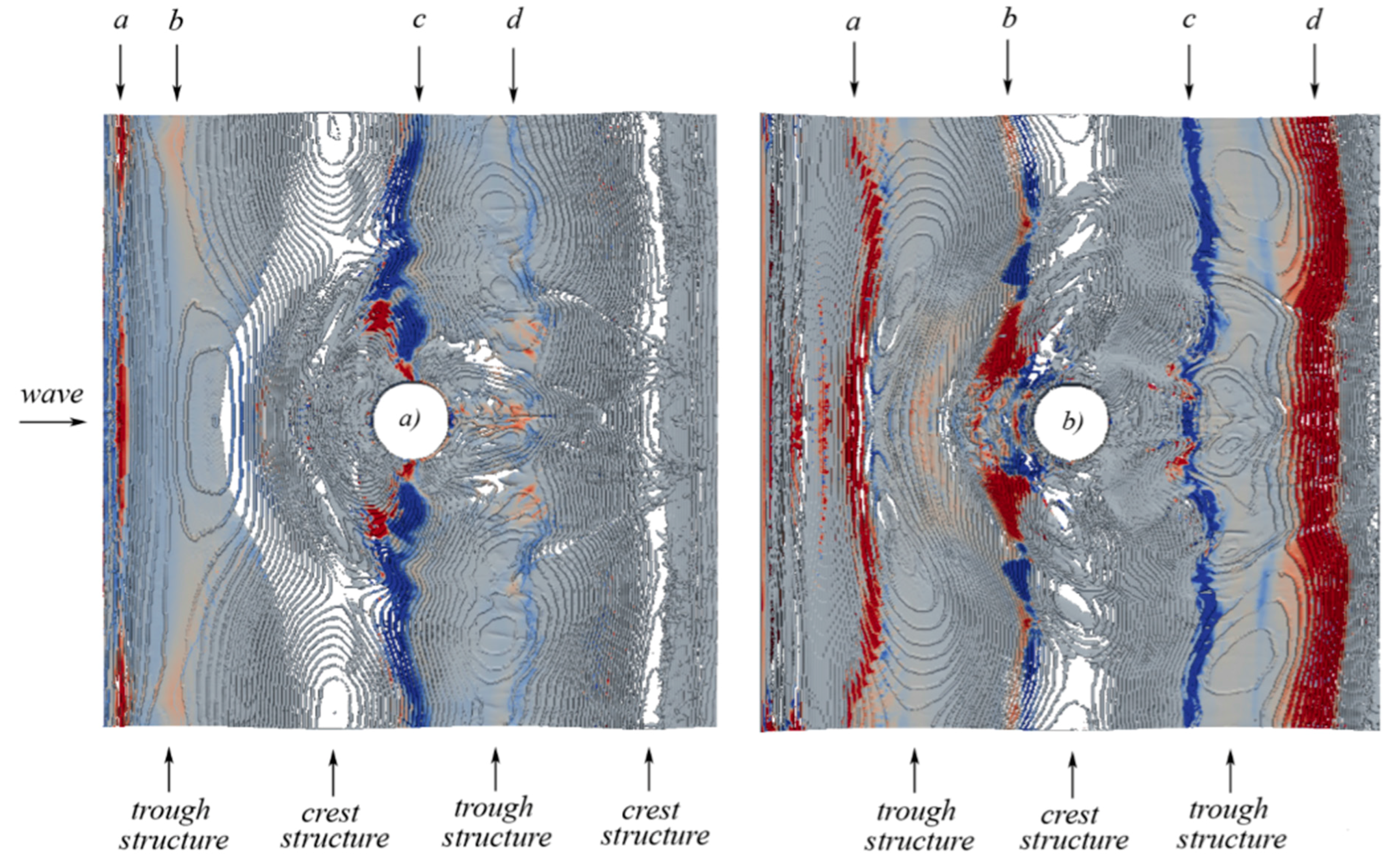
5.4. Navier Stokes Equations

As a result of the computing procedures previously outlined (Section 3.3), results related to the Navier-Stokes-equations-derived flow fields, are presented (as for the kind of information incorporated in the following figures, one can refer to the previous section).
Figure 18a,b show top views of the computing domain at t = t F max N S (the instant at which the Navier-Stokes-derived wave field exerts the maximum force on the cylinder), and t = t R max N S (the instant at which the Navier-Stokes-derived wave field exhibits the maximum runup on the external surface of the cylindrical body), respectively.
The fields are rather regular and substantially symmetric, and the structure field exhibits a number of tubular and—in this case—mainly flattened vortical structures, concentrated at the free surface. Again, from the distribution of these structures, one obtains the perception of the free-surface configuration in terms of wave crests and troughs, and also of the accumulation of fluid mass upstream from the cylinder, and the progressive development of the wave-diffraction phenomenon related to the wave-cylinder interaction process (lines a to q in Figure 18). The nature of the free-surface flattened (viscous) tubular structures is that of being predominantly irrotational far away from the cylinder, though becoming rotational when they actually interact with the cylindrical body. Moreover, the flattened structures tend to stay irrotational in their free-surface portion, while becoming rotational immediately under the free surface. This is due to the presence of a negligible shear-stress field at the free surface, and to a non-negligible shear-stress-field under the free surface.
Figure 18. Flow structures as obtained from the solution of the primitive-variable Navier-Stokes equations. Top view of free-surface profile: (a) t = t F max N S ; (b) t = t R max N S .
Computation 03 00386 g018
The structure fields shown in Figure 18 also exhibit a number of strong and not flattened tubular structures immediately under the free surface, mainly located upstream from the cylinder, that represent the underwater consequence of the manifestation of the wave troughs at the free surface in their viscous interaction with the cylindrical body. An inspection to Figure 18 also shows that, through the field, zones characterized by more and/or less intense coloring (either reddish or bluish) are present in the field, and also that, typically at the free surface, a more intense ω y coloring (either reddish or bluish) mainly verifies in the vicinity of the wave troughs. This latter phenomenon is due to the presence of the above-mentioned strongly-rotational underwater tubular structures, whose vorticity field breaks up the predominantly-irrotational character of the structures at the free-surface.
Moreover, from Figure 18a, at t = t F max N S , one can notice that the presence of the cylindrical body induces an inversion in the sign of ω y in the trough immediately upstream from the cylinder (from reddish to bluish in front of the cylinder), being the latter bluish zone progressively pushed towards the boundaries of the domain at t = t R max N S (Figure 18b). What happens there is that the presence of the cylindrical body in front of the ascending portion of the wave determines an inversion of the fluid-particle orbital paths, with the consequence that the shear-stress field induces a strong negative ω y -field in the zone right in front of the cylinder.
In Figure 19, Figure 20 and Figure 21, upstream-, side- and downstream-close-up views of the structure field are shown in the vicinity of the cylinder external wall, at t = t F max N S , and t = t R max N S , respectively. From these figures it can be noticed that other types of viscous-flow structures develop under the free surface. The establishment of the latter structures actually represents the more relevant difference between the Navier-Stokes- (and/or eventually Euler-) flow-fields, and the velocity-potential-derived flow fields, so unveiling physical phenomena that are impossible to detect by only analyzing the potential-derived fields.
Figure 19, Figure 20 and Figure 21 show first—as also previously mentioned—the presence of two main underwater tubular, not flattened structures upstream from the cylinder and under the wave trough, characterized by high positive vorticity. In going from t = t F max N S to t = t R max N S these structures grow in dimensions, and the one that is nearest to the cylinder develops a more extended, massive sub-structure, right in front of the cylinder itself. These structures in the whole represent the underwater consequence of the manifestation of the trough at the free surface, where the aforementioned more extended sub-structure represents the underwater counterpart of the wave-to-cylinder approaching process.
Figure 19. Close-up at the cylinder surface of viscous-flow structures as obtained from the solution of the Navier-Stokes equations. Upstream view: (a) t = t F max N S ; (b) t = t R max N S .
Computation 03 00386 g019
Figure 20. Close-up at the cylinder surface of viscous-flow structures as obtained from the solution of the Navier-Stokes equations. Side view: (a) t = t F max N S ; (b) t = t R max N S .
Computation 03 00386 g020
Figure 21. Close-up at the cylinder surface of viscous-flow structures as obtained from the solution of the Navier-Stokes equations. Downstream view: (a) t = t F max N S ; (b) t = t R max N S .
Computation 03 00386 g021
Additional and differently-shaped flow structures are present in the underwater environment nearby the cylinder at both t = t F max N S and t = t R max N S . In Figure 19, Figure 20 and Figure 21, arrow 1 indicates a structure that completely encompasses the cylindrical body. At t = t F max N S , structure 1 is characterized by strong negative vorticity on the cylinder downstream side, by strong positive vorticity laterally, and by an additional-structure superposition phenomenon (structures 2 and 3) on the upstream side. Structure 2 is characterized by high values of positive vorticity, while structure 3 is characterized by less intense ω y (Figure 19a). Moreover, through Figure 19, Figure 20 and Figure 21, arrows 4 and 5 indicate flow structures that develop respectively upstream (structure 4) and downstream (structure 5) from the cylinder, immediately under the free-surface level. Structure 4 appears to be the underwater counterpart of the phenomenon of accumulation of fluid mass that verifies upstream from the cylinder when the wave approaches the cylindrical body. Structure 5 appears as being the downstream underwater remnant of the cylinder-wave interaction process.
Overall, both structure field and vorticity field strongly change in going from t = t F max N S to t = t R max N S . While at t = t F max N S the underwater field is populated by structures 1, 2, 3, 4, 5, at t = t R max N S , structures 2 and 3 have disappeared, structure 1 is characterized by strong positive ω y on the cylinder upstream side (exception made for a small central area, Figure 19b), structure 4 has separated in two portions and changed the sign of ω y (Figure 19b), while on the cylinder downstream side, structure 5 still persists, though smaller than previously (Figure 21b).
Additional information on the phenomenon at hand can be derived from specific structure-field representations. Figure 22 and Figure 23 show close-ups of the structure field (block 3 of the computational domain, Figure 9), at t = t F max N S and t = t R max N S , respectively.
The left portion of each of these figures represents a bottom close-up view of the structure field, as represented with the same criterion previously used, such that the external surfaces of the flow structures are colored with the values assumed by the spanwise component of the vorticity ( ω y , reddish areas denote positive ω y , bluish areas denote negative ω y , greyish areas denote zero ω y , more intense coloring corresponds to high ω y -values, less intense coloring corresponds to lower ω y -values). The right portions of Figure 22 and Figure 23 also represents the structure field at t = t F max N S and t = t R max N S , where now the external surfaces of the structures are colored with the values assumed by the pressure, in a darker-to-lighter color scale (bluish areas denotes low values of the pressure, in the vicinity of the free surface, rosy areas denote higher values of the pressure, more deep under the free surface).
Figure 22. Close-up views of structures as obtained from the solution of the Navier-Stokes equations. Bottom view of computing domain at t = t F max N S . The external surfaces of structures are colored with: (a) wave-field spanwise vorticity; (b) wave-field pressure values.
Computation 03 00386 g022
Figure 23. Close-up views of structures as obtained from the solution of the Navier-Stokes equations. Bottom view of computing domain at t = t R max N S . The external surfaces of structures are colored with: (a) wave-field spanwise vorticity; (b) wave-field pressure values.
Computation 03 00386 g023
The following can be observed.
In Figure 22a it is possible first to observe some phenomena already depicted in Figure 18a, namely the existence—upstream from the cylinder—of a spanwise tubular (not flattened) structure, as part of a more complex wave-trough flow structure, that includes the vorticity-inversion zone at center, in front of the cylinder. It also to be noted how the intensity of the vorticity field under the free-surface level is higher upstream from cylinder than downstream). Figure 22b further shows that the peripheral portion of the above-mentioned tubular structure lies more in depth (lighter-blue areas in Figure 22b near the boundaries of the computing domain) than its central part.
Figure 22 also shows the presence of structure 4 (see also at Figure 19 and Figure 20). This structure, at t = t F max N S , is characterized by negative vorticity (Figure 22a), and by a remarkable depth just in front of the cylinder (Figure 22b). Other structures are detectable, especially in Figure 22a, namely those already characterized by lines k, l, m, n, o, p, q in Figure 18a. This is the structural character of the flow field in the vicinity of the cylinder, at the time at which the wave exerts the maximum force on the obstacle.
Figure 23 shows the flow-field representation at the time at which the wave exhibits the maximum runup on the external surface of the cylindrical body. Also here (see also at Figure 18b) a complex tubular structure can be recognized upstream form the cylinder in Figure 23a, that exhibits—in its central part—a massive sub-structure just in front of the cylinder. Note how this sub-structure is characterized by less intense vorticity with respect to other portions of the same structure. From Figure 23b can be also observed that the new sub-structure, and its adjacent portions, extend remarkably in deep under the free surface, in a difference with respect to what shown in Figure 22b (at the previous instant), where the central portion of the structure upstream from the cylinder lied, in practice, at the free-surface level. Figure 23 also shows the presence of structure 4 (see also at Figure 19 and Figure 20) as characterized—this time—by positive vorticity (Figure 23a, the structure has broken-up in two parts), and, again, by a remarkable depth under the free-surface, in front of the cylinder (Figure 23b).
Further, as a result of the computing procedures previously outlined (Section 4.2), results in terms of proper orthogonal flow modes are presented. Top views (the free-surface level) of a reconstructed velocity field, based on the three most energetic eignefunctions of the decomposition, are shown in Figure 24, Figure 25, Figure 26, Figure 27 and Figure 28, in terms of constant wave-flow x-velocity, through a time interval equal to a wave period, in a comparison with the structure field (same computing subdomain).
Figure 24a ( T = 0.000 , T is the wave period) shows that, at the beginning of the wave period (the oncoming wave is only slightly altered by the presence of the cylinder), the free surface is mainly irrotational. On the upstream side of the cylinder, the diffraction tracks are clearly detectable in terms of borders among structures, where track a denotes the ascending portion of the wave, track b denotes the wave crest, and track e denotes the still-water level (note that, due to the particular nature of information incorporated in these figures, the track lettering is now different from that adopted in Figure 18). Only very small zones of positive (reddish) spanwise vorticity are present, immediatly upstream from the cylinder, at the cylinder wall. Overall, the field is regular and symmetric. Figure 24b shows the flow field in terms of KL modes. It can be first noted that there is no direct correspondence between the field visualized in Figure 24a and that shown in Figure 24b, meaning that the energy content of the flow distributes through the field with no direct correspondence with the topological-structure distribution. The only similarity between the two visualizations is mirrored by the position of track a, also indicated in Figure 24b.
Figure 24. Flow-field representation at T = 0.000 (T is wave period), top view (free-surface level): (a) flow-structures (colored with spanwise vorticity); (b) surfaces of constant x-velocity from reconstruction based on the three most energetic KL modes.
Computation 03 00386 g024
Figure 25. Flow-field representation at T = 0.144 (T is wave period), top view (free-surface level): (a) flow-structures (colored with spanwise vorticity); (b) surfaces of constant x-velocity from reconstruction based on the three most energetic KL modes.
Computation 03 00386 g025
Further upstream from track a, in Figure 24b, other tracks are present (oblique arrows) that actually represent borders between flow structures with high kinetic-energy content. A further inspection to Figure 24b shows that the field upstream from the cylinder can be seen as divided in two zones, namely a first zone right in front of the obstacle, characterized by remarkably-small flow scales, and a second zone characterized by larger scales. A flow-mode border is also detectable in Figure 24b, between these two zones of high-kinetic-energy scale-organization. In Figure 25a,b the fields at T = 0.144 are represented. Figure 25a shows the evolution of the diffraction tracks with respect to the previous instant. On the upstream side of the cylinder, track d denotes the descending portion of the wave, track e is now interrupted by track f, and track g now denotes the presence in the field of the already mentioned rather complex wave trough. This latter g-structure actually mirrors the previously-outlined vorticity-inversion phenomenon in front of the cylinder (this section). Also in this case, the only detectable similarity between the visualization of Figure 25a and that of Figure 25b is the position of track d, also indicated in Figure 25b. Again, further upstream from track d, in Figure 25b, other tracks are present (oblique arrows), representing borders between flow structures with high kinetic-energy content, and a further inspection to Figure 25b shows that the field upstream from the cylinder is also divided in two zones, i.e., a first zone characterized by small flow scales, and a second zone characterized by larger flow scales. A flow-mode border also appears in Figure 25b, between these two zones of high-kinetic-energy scale-organization. In Figure 26a,b the fields at T = 0.500 are represented. Figure 26a shows again the evolution of the diffraction tracks with respect to the previous instant. On the upstream side of the cylinder, tracks f and g have in practice collapsed into a unique structure (now approaching the cylinder), tracks h and i denote the ascending portion of the wave (toward the crest), while track k indicates the presence of a new crest in the domain. Also in this case, the only detectable similarity between the visualization of Figure 26a and that of Figure 26b, is the position of track f, and, again, further upstream from track f, in Figure 26b, other tracks are present (oblique arrows), representing borders between structures with high kinetic-energy content. A further inspection to Figure 26b shows that the field upstream from the cylinder is again divided in two zones, a first small-scale zone, and a second large-scale zone, and a flow-mode border is again detectable in Figure 26b. It can be noted that the presence of the aforementioned discontinuity between smaller and larger high-kinetic-energy flow scales (and mirrored by the presence of a distinct flow-mode border) lasts from T = 0.000 up to T = 0.500 i.e., in practice, along the whole wave-to-cylinder approaching phase. In Figure 27a,b the fields at T = 0.750 are represented. In Figure 27a, on the cylinder upstream side, track i clearly mirrors the interaction between wave and cylinder, while the wave-crest track k is approaching the cylinder, assuming, at the same time, a complex configuration in front of the cylinder. In this case, the only detectable similarity between the fields represented respectively in Figure 27a,b, is track i, while, in Figure 27b, other tracks are present (oblique arrows), always representing borders between flow structures with high kinetic-energy content. Differently from the previous instants, it clearly appears from Figure 27b, that no more discontinuities between smaller and larger high-kinetic-energy flow scales are present, and the field of high-energy scales continuously evolves from the center to the periphery of the domain, in forming an elongated pattern. In Figure 28a,b the fields at T = 1.000 are represented. In Figure 28a, on the cylinder upstream side, the crest-track k is now approaching the cylinder, while tracks l and m denote the descending portion of the wave. The configuration of the high-energy scales of Figure 28b is similar to that of the previous instant, where the similarity between the two fields can be now recognized in the position of track k.
Overall, the flow fields (actually the iso-u-fields) that have been reconstructed by using the three most energetic eigenfunctions of the KL decomposition, further show that the borders of the flow structures are actually borders among high-energy flow structures of tubular nature, the latter appearing—with respect to their energy content—the most significant type of viscous-flow structures that have been found in the wave-cases considered in the present work.
Figure 26. Flow-field representation at T = 0.500 (T is wave period), top view (free-surface level): (a) flow-structures (colored with spanwise vorticity); (b) surfaces of constant x-velocity from reconstruction based on the three most energetic KL modes.
Computation 03 00386 g026
Figure 27. Flow-field representation at T = 0.750 (T is wave period), top view (free-surface level): (a) flow-structures (colored with spanwise vorticity); (b) surfaces of constant x-velocity from reconstruction based on the three most energetic KL modes.
Computation 03 00386 g027
Figure 28. Flow-field representation at T = 1.000 (T is wave period), top view (free-surface level): (a) flow-structures (colored with spanwise vorticity); (b) surfaces of constant x-velocity from reconstruction based on the three most energetic KL modes.
Computation 03 00386 g028

6. Concluding Remarks

In the present work, the phenomenon of diffraction of linear waves impinging on large-diameter, surface-piercing, vertical circular cylinder has been investigated numerically, within three different theoretical frameworks of hypotheses, namely the velocity potential, the numerical integration of the primitive-variable Euler equations, and the numerical integration of the primitive-variable Navier-Stokes equations (with the DNS approach). The results obtained in terms of both global wave parameters (forces and runups), and wave-flow fields have shown that remarkable differences exist, depending on the frame of hypotheses that one eventually choses to follow, being though the numerical integration of the full Navier-Stokes equations in primitive variables (the velocity-pressure formulation) the physically-consistent approach to be adopted to obtain flow fields that correctly represent the numerical equivalent of the phenomena at hand. More in particular, as related to the calculation of forces and runups on the cylindrical body, it has been found that the agreement between the values obtained from the numerical integration of the Euler equations and the potential-theory results is rather good, showing that when inviscid fluids are considered, both potential theory and primitive-variable mass- and momentum-conservation equations, give in practice the same results. Thus, all the differences that one finds between inviscid-fluid- and viscous-fluid results (as related in particular to the maximum runup) have to be correctly attributed to the effects of the real-fluid, viscosity-generated shear-stress field. With reference to the wave-flow fields, in the case of the velocity potential approach, no flow structures appear in the field as a result of the wave-cylinder interaction process (as expected), due to the pure-mathematical nature of the latter approach. In the case of the Euler-equations-derived flow fields, flow structures actually appear, in particular contaminated by a previously-generated spanwise vorticity that conservatively evolves with time. Finally, in the case of the Navier-Stokes-equations-derived flow fields, complex flow structures of physical nature appear, as extracted with both the swirling-strength criterion, and the Karhunen-Loève decomposition technique.

Conflicts of Interest

The author declares no conflicts of interest.

Nomenclature

Roman Symbols (Upper Case)

A i j
velocity-gradient tensor
D
cylinder diameter
Dsc
discriminant of characteristic equation
F f
portion-due-to-friction of force on cylinder
F max
maximum force on cylinder
F max n d
maximum force on cylinder (nondimensional)
H
wave height
H p ( 1 )
Hankel function of first kind (order p)
H p ( 1 )
first derivative of H p ( 1 )
J p
Bessel function of first kind (order p)
J p
first derivative of J p
KC
Keulegan-Carpenter number
L
wave length
L x , L y , L z
dimensions of computing domain along (x,y,z)
L x + , L y + , L z +
dimensions of computing domain along (x,y,z) in wall units (test case)
N x , N y , N z
number of grid points in the computing domain along (x,y,z)
N t o t
total number of grid points in the computing domain
P,Q,R
scalar invariants of velocity-gradient tensor
PP
parameter in hyperbolic-tangent grid-stretching law
QQ
parameter in hyperbolic-tangent grid-stretching law
R max
maximum runup at cylinder surface
R max n d
maximum runup at cylinder surface (nondimensional)
Re
wave-field Reynolds number
Re N S
Reynolds number resulting from nondimensionalization of Navier-Stokes equations
Re τ
friction-velocity Reynolds number (test case)
T
wave period
Y p
Bessel function of second kind (order p)
Y p
first derivative of Y p

Roman Symbols (Lower Case)

a
wave amplitude
d
still-water level
g
acceleration due to gravity ( g = 9.807 m / s 2 )
h
channel half-width (test case)
k
wavenumber
p
pressure (also index)
real
real part of complex quantity
r, θ ,z
cylindrical coordinate system
r 0
cylinder radius
t
time coordinate
t F m a x E u l e r
time at which the Euler-equations-derived F max verifies
t R m a x E u l e r
time at which the Euler-equations-derived R max verifies
t F max N S
time at which the Navier-Stokes-equations-derived F max verifies
t R max N S
time at which the Navier-Stokes-equations-derived R max verifies
t F max φ
time at which the φ -derived F max verifies
t R max φ
time at which the φ -derived R max verifies
u i ( u , v , w )
velocity components along (x,y,z)
u i ( u , v , w )
fluctuating-velocity components along (x,y,z) (test case)
u max
maximum value of u
x i ( x , y , z )
cartesian coordinates (x is wave direction, z is vertical direction)

Greek Symbols (Upper Case)

Δ t
time resolution of calculations
Δ x , Δ y , Δ z
space resolution of calculations along (x,y,z)

Greek Symbols (Lower Case)

β
Re / K C
δ
phase angle
δ i j
Kronecker delta
ε ¯
average rate of dissipation of kinetic energy per unit mass
ε i j k
alternating-unit tensor
λ
eigenvalue
λ r
real eigenvalue
λ c r
real part of complex eigenvalue
λ c i
imaginary part of complex eigenvalue pair (swirling strength)
( λ c i ) t h
threshold value of swirling strength
η
Kolmogorov length scale
ν
fluid kinematic viscosity
τ w
mean shear stress at the wall
τ η
Kolmogorov time scale
φ
velocity-potential
ρ
fluid density
ω
wave angular frequency
ω i
vorticity vector
ω y
spanwise component of vorticity

Acronyms (Upper Case)

ADI
Alternating Direction Implicit (scheme)
DNS
Direct Numerical Simulation (technique)
FAVOR
Fractional Area Volume Obstacle Representation (technique)
GMRES
Generalized Minimal Residual (method)
KL
Karhunen-Loève (decomposition technique)
RANS
Reynolds Averaged Navier-Stokes (equations)
RNG
Renormalization Group (theory)
VOF
Volume Of Fluid (method)

Acronyms (Lower Case)

lhs
left-hand side (of equation)
rhs
right-hand side (of equation)

References

  1. MacCamy, R.C.; Fuchs, R.A. Wave forces on piles: A diffraction theory. Available online: http://acwc.sdp.sirsi.net/client/search/asset/1007800 (accessed on 25 August 2015).
  2. Mansour, A.M.; Williams, A.N.; Wang, K.H. The diffraction of linear waves by a uniform vertical cylinder with cosine-type radial perturbations. Ocean Eng. 2002, 29, 239–259. [Google Scholar] [CrossRef]
  3. Roy, P.D.; Ghosh, S. Wave force on vertically submerged circular thin plate in shallow water. Ocean Eng. 2006, 33, 1935–1953. [Google Scholar] [CrossRef]
  4. Kim, N.H.; Park, M.S.; Yang, S.B. Wave force analysis of vertical circular cylinder by boundary element method. KSCE J. Civil Eng. 2007, 11, 31–35. [Google Scholar] [CrossRef]
  5. Helstrom, B.; Rundgren, L. Model tests on Oland Sodva Grund light-house. Available online: https://www.kth.se/en (accessed on 27 August 2015).
  6. Laird, A.D.K. A model study of wave action on a cylindrical island. Trans. Am. Geoph. Union 1955, 26, 279–285. [Google Scholar] [CrossRef]
  7. Bonnefille, R.; Germain, P. Wave Action on isolated Vertical Cylinders of Large Dimension; IAHR Congress: London, UK, 1963. [Google Scholar]
  8. Isaacson, M. Wave runup around large circular cylinder. ASCE J. Waterw. Harb. Coast. Eng. Div. 1978, 104, 69–79. [Google Scholar]
  9. Galvin, C.J.; Hallermeier, R.J. Wave run-up on vertical cylinders. In Proceedings of the 13th ASCE International Conference Coastal Engineering, Vancouver, BC, Canada, 10–14 July 1972; pp. 1955–1974.
  10. Hallermeier, R.J. Nonlinear flow of wave crests past a thin pile. ASCE J. Waterw. Harb. Coast. Eng. Div. 1976, 102, 365–377. [Google Scholar]
  11. Haney, J.P.; Herbich, J.B. Wave flow around thin piles and pile groups. J. Hydr. Res. 1982, 20, 1–14. [Google Scholar] [CrossRef]
  12. Chakrabarti, S.; Tam, W.A. Wave height distribution around vertical cylinder. ASCE J. Waterw. Harb. Coast. Eng. Div. 1975, 101, 225–230. [Google Scholar]
  13. Niedzwecki, J.M.; Duggal, A.S. Wave run-up and wave forces on a truncated cylinder. In Proceedings of the 22nd Offshore Technology Conference, Houston, TX, USA, 7–10 May 1990; pp. 593–600.
  14. Niedzwecki, J.M.; Duggal, A.S. Wave run-up and forces on cylinders in regular and random waves. ASCE J. Waterw. Port Coast. Ocean Eng. 1992, 118, 615–632. [Google Scholar] [CrossRef]
  15. Niedzweki, J.M.; Huston, J.R. Wave interaction with tension leg platforms. Ocean Eng. 1992, 19, 21–37. [Google Scholar] [CrossRef]
  16. Martin, A.J.; Easson, W.J.; Bruce, T. Runup on columns in steep, deep water regular waves. ASCE J. Waterw. Port Coast. Ocean Eng. 2001, 127, 26–32. [Google Scholar] [CrossRef]
  17. Mase, H.; Kosho, K.; Nagahashi, S. Wave runup of random waves on a small circular pier on sloping seabed. ASCE J. Waterw. Port Coast. Ocean Eng. 2001, 127, 192–199. [Google Scholar] [CrossRef]
  18. Morris-Thomas, M.T.; Thiagarajan, K.P. The run-up on a cylinder in progressive surface gravity waves: harmonic components. Appl. Ocean Res. 2004, 26, 98–113. [Google Scholar] [CrossRef]
  19. De Vos, L.; Frigaard, P.; de Rouck, J. Wave run-up on cylindrical and cone shaped foundations for offshore wind turbines. Coast. Eng. 2007, 54, 17–29. [Google Scholar] [CrossRef]
  20. Choi, B.H.; Kim, D.C.; Pelinovsky, E.; Woo, S.B. Three-dimensional simulation of tsunami run-up around conical island. Coast. Eng. 2007, 54, 618–629. [Google Scholar] [CrossRef]
  21. Alfonsi, G. Reynolds-averaged Navier-Stokes equations for turbulence modeling. Appl. Mech. Rev. 2009, 62, 040802. [Google Scholar] [CrossRef]
  22. Alfonsi, G. Results of numerical integration of the Navier-Stokes equations in the field of direct simulation of turbulence. J. Flow Vis. Image Proc. 2011, 18, 91–135. [Google Scholar] [CrossRef]
  23. Alfonsi, G. On direct numerical simulation of turbulent flows. Appl. Mech. Rev. 2011, 64, 020802. [Google Scholar] [CrossRef]
  24. Sarpkaya, T.; Isaacson, M. Mechanics of Wave Forces in Offshore Structures; Van Nostrand Reinhold: New York, NY, USA, 1981. [Google Scholar]
  25. Isaacson, M. Wave induced forces in the diffraction regime. In Mechanics of Wave-Induced Forces on Cylinders; Pitman: London, UK, 1979. [Google Scholar]
  26. Honji, H. Streaked flow around an oscillating circular cylinder. J. Fluid Mech. 1981, 107, 509–520. [Google Scholar] [CrossRef]
  27. Sarpkaya, T. Force on a circular cylinder in viscous oscillatory flow at low Keulegan-Carpenter numbers. J. Fluid Mech. 1986, 165, 61–71. [Google Scholar] [CrossRef]
  28. Sumer, B.M.; Fredsøe, J. Hydrodynamics around Cylindrical Structures; World Scientific: Singapore, 1999. [Google Scholar]
  29. Hirt, C.W.; Nichols, B.D. Volume of fluid (VOF) method for the dynamics of free boundaries. J. Comput. Phys. 1981, 39, 201–225. [Google Scholar] [CrossRef]
  30. Flow-3D User Manual; Flow Science, Inc.: Santa Fe, NM, USA, 2004.
  31. Alfonsi, G.; Ciliberti, S.A.; Mancini, M.; Primavera, L. Performances of Navier-Stokes solver on a hybrid CPU/GPU computing system. Lect. Notes Comp. Sci. 2011, 6873, 404–416. [Google Scholar]
  32. Alfonsi, G.; Ciliberti, S.A.; Mancini, M.; Primavera, L. GPGPU implementation of mixed spectral-finite difference computational code for the numerical integration of the three-dimensional time-dependent incompressible Navier-Stokes equations. Comp. Fluids 2014, 102, 237–249. [Google Scholar] [CrossRef]
  33. Alfonsi, G.; Muttoni, L. Performance evaluation of a Windows NT based PC cluster for high performance computing. J. Syst. Arch. 2004, 50, 345–359. [Google Scholar] [CrossRef]
  34. Alfonsi, G. Analysis of time dependent vortex shedding by means of streamfunctions’ strictly rotational component. J. Flow Vis. Image Proc. 2003, 10, 67–103. [Google Scholar]
  35. Alfonsi, G. Unsteady development of vortical structures in the symmetric near wake of a cylinder. J. Flow Vis. Image Proc. 2005, 12, 45–72. [Google Scholar]
  36. Alfonsi, G. Numerical visualization of unsteady vortex shedding. J. Flow Vis. Image Proc. 2005, 12, 105–110. [Google Scholar] [CrossRef]
  37. Alfonsi, G.; Giorgini, A. Nonlinear perturbation of the vortex shedding from a circular cylinder. J. Fluid Mech. 1991, 222, 267–291. [Google Scholar]
  38. Alfonsi, G.; Giorgini, A. Temporal evolution of high-order vortices in the nonsymmetric wake of a circular cylinder. Fluid Dyn. Res. 2002, 31, 13–39. [Google Scholar]
  39. Alfonsi, G. Coherent structures of turbulence: methods of eduction and results. Appl. Mech. Rev. 2006, 59, 307–323. [Google Scholar]
  40. Alfonsi, G. Techniques of research and results in the field of coherent structures of wall-bounded turbulence. In Vorticity Turbulence Effects Fluid Structure Interaction; Wessex Institute of Technology Press: Southampton, UK, 2006; pp. 1–27. [Google Scholar]
  41. Kocaman, S.; Seckin, G.; Erduran, K.S. 3D model for prediction of flow profiles around bridges. J. Hydr. Res. 2010, 48, 521–525. [Google Scholar] [CrossRef]
  42. Cho, S.M. Foundation design of the Incheon bridge. Geotech. Eng. J. 2010, 41, 1–16. [Google Scholar]
  43. Jin, J.; Meng, B. Computation of wave loads on the superstructures of coastal highway bridges. Ocean Eng. 2011, 38, 2185–2200. [Google Scholar] [CrossRef]
  44. Kim, C.; Kim, J.; Kang, J. Analysis of the cause for the collapse of a temporary bridge using numerical simulation. Sci. Res. 2013, 5, 997–1005. [Google Scholar] [CrossRef]
  45. Kayser, M.; Gabr, M.A. Assessment of scour on bridge foundations by means of in situ erosion evaluation probe. J. Transp. Res. Board 2013, 2335, 72–78. [Google Scholar] [CrossRef]
  46. Alfonsi, G.; Passoni, G.; Pancaldo, L.; Zampaglione, D. A spectral-finite difference solution of the Navier-Stokes equations in three dimensions. Int. J. Numer. Meth. Fluids 1998, 28, 129–142. [Google Scholar] [CrossRef]
  47. Passoni, G.; Alfonsi, G.; Tula, G.; Cardu, U. A wavenumber parallel computational code for the numerical integration of the Navier-Stokes equations. Parall. Comp. 1999, 25, 593–611. [Google Scholar] [CrossRef]
  48. Passoni, G.; Cremonesi, P.; Alfonsi, G. Analysis and implementation of a parallelization strategy on a Navier-Stokes solver for shear flow simulations. Parall. Comp. 2001, 27, 1665–1685. [Google Scholar] [CrossRef]
  49. Passoni, G.; Alfonsi, G.; Galbiati, M. Analysis of hybrid algorithms for the Navier-Stokes equations with respect to hydrodynamic stability theory. Int. J. Numer. Meth. Fluids 2002, 38, 1069–1089. [Google Scholar] [CrossRef]
  50. Alfonsi, G.; Primavera, L. Direct numerical simulation of turbulent channel flow with mixed spectral-finite difference technique. J. Flow Vis. Image Proc. 2007, 14, 225–243. [Google Scholar]
  51. Mochizuki, S.; Nieuwstadt, F.T.M. Reynolds-number-dependence of the maximum of the streamwise velocity fluctuations in wall turbulence. Exp. Fluids 1996, 21, 218–226. [Google Scholar] [CrossRef]
  52. Alfonsi, G. Analysis of streamwise velocity fluctuations in turbulent pipe flow with the use of an ultrasonic Doppler flowmeter. Flow Turbul. Combust. 2001, 67, 137–142. [Google Scholar] [CrossRef]
  53. Xu, C.; Zhang, Z.; den Toonder, J.M.J.; Nieuwstadt, F.T.M. Origin of high kurtosis level in the viscous sublayer. Direct numerical simulation and experiment. Phys. Fluids 1996, 8, 1938–1944. [Google Scholar] [CrossRef]
  54. Alfonsi, G. Evaluation of radial velocity fluctuations in turbulent pipe flow by means of an ultrasonic Doppler velocimeter. J. Flow Vis. Image Proc. 2003, 10, 155–161. [Google Scholar] [CrossRef]
  55. Alfonsi, G.; Brambilla, S.; Chiuch, D. The use of an ultrasonic Doppler velocimeter in turbulent pipe flow. Exp. Fluids 2003, 35, 553–559. [Google Scholar] [CrossRef]
  56. Alfonsi, G.; de Bartolo, S.; Gaudio, R.; Primavera, L. Reliability of 5-beam LDV fiberoptic probe for turbulence measurements in the wall region of open channel flow. J. Flow Vis. Image Proc. 2009, 16, 255–277. [Google Scholar] [CrossRef]
  57. Bakewell, H.P.; Lumley, J.L. Viscous sublayer and adjacent wall region in turbulent pipe flow. Phys. Fluids 1967, 10, 1880–1889. [Google Scholar] [CrossRef]
  58. Bearman, P.W.; Downie, M.J.; Graham, J.M.R.; Obasaju, E.D. Forces on cylinders in viscous oscillatory flow at low Keulegan-Carpenter numbers. J. Fluid Mech. 1985, 154, 337–356. [Google Scholar] [CrossRef]
  59. Morison, J.R.; O’Brien, M.P.; Johnson, J.W.; Shaag, S.A. The forces exerted by surface waves on piles. AIME J. Petrol. Technol. 1950, 189, 149–154. [Google Scholar] [CrossRef]
  60. Alfonsi, G.; Primavera, L. Vortex identification in the wall region of turbulent channel flow. Lect. Notes Comp. Sci. 2007, 4487, 9–16. [Google Scholar]
  61. Alfonsi, G.; Primavera, L. On identification of vortical structures in turbulent shear flow. J. Flow Vis. Image Proc. 2008, 15, 201–216. [Google Scholar]
  62. Zhou, J.; Adrian, R.J.; Balachandar, S.; Kendall, T.M. Mechanisms for generating coherent packets of hairpin vortices in channel flow. J. Fluid Mech. 1999, 387, 353–396. [Google Scholar] [CrossRef]
  63. Alfonsi, G. On vorticity-field evolution in viscous- and inviscid-fluid wave-diffraction cases. J. Flow Vis. Image Proc. 2013, 20, 209–225. [Google Scholar]
  64. Alfonsi, G.; Primavera, L. Determination of the threshold value of the quantity chosen for vortex representation in turbulent flow. J. Flow Vis. Image Proc. 2009, 16, 41–49. [Google Scholar]
  65. Alfonsi, G.; Primavera, L. Temporal evolution of vortical structures in the wall region of turbulent channel flow. Flow Turbul. Comb. 2009, 83, 61–79. [Google Scholar] [CrossRef]
  66. Alfonsi, G.; Ciliberti, S.A.; Mancini, M.; Primavera, L. Hairpin vortices in turbulent channel flow. Proc. Comp. Sci. 2011, 4, 801–810. [Google Scholar] [CrossRef]
  67. Alfonsi, G.; Ciliberti, S.A.; Mancini, M.; Primavera, L. Turbulent events in a wall-bounded turbulent flow. J. Flow Vis. Image Proc. 2012, 19, 139–160. [Google Scholar]
  68. Alfonsi, G.; Lauria, A.; Primavera, L. Flow structures around a large-diameter circular cylinder. J. Flow Vis. Image Proc. 2012, 19, 15–35. [Google Scholar] [CrossRef]
  69. Alfonsi, G.; Lauria, A.; Primavera, L. Structures of a viscous-wave flow around a large-diameter circular cylinder. J. Flow Vis. Image Proc. 2012, 19, 323–354. [Google Scholar]
  70. Alfonsi, G.; Lauria, A.; Primavera, L. A study of vortical structures past the lower portion of the Ahmed car model. J. Flow Vis. Image Proc. 2012, 19, 81–95. [Google Scholar]
  71. Liang, Y.C.; Lee, H.P.; Lim, S.P.; Lin, W.Z.; Lee, K.H.; Wu, C.G. Proper orthogonal decomposition and its applications, Part I: Theory. J. Sound Vibr. 2002, 252, 527–544. [Google Scholar]
  72. Lumley, J.L. Stochastic Tools in Turbulence; Academic Press: New York, NY, USA, 1971. [Google Scholar]
  73. Sirovich, L. Turbulence and the dynamics of coherent structures, Part I: Coherent structures, Part II: Symmetries and transformations, Part III: Dynamics and scaling. Quart. Appl. Math. 1987, 45, 561–590. [Google Scholar]
  74. Alfonsi, G.; Primavera, L. Coherent structure dynamics in turbulent channel flow. J. Flow Vis. Image Proc. 2002, 9, 89–98. [Google Scholar]
  75. Alfonsi, G.; Primavera, L. Description of turbulent events trough the analysis of POD modes in numerically simulated turbulent channel flow. Lect. Notes Comp. Sci. 2005, 3514, 623–630. [Google Scholar]
  76. Alfonsi, G.; Primavera, L. Dynamics of POD modes in wall-bounded turbulent flow. Lect. Notes Comp. Sci. 2006, 3991, 465–472. [Google Scholar]
  77. Alfonsi, G.; Primavera, L. The structure of turbulent boundary layers in the wall region of plane channel flow. Proc. R. Soc. A 2007, 463, 593–612. [Google Scholar] [CrossRef]
  78. Alfonsi, G.; Lauria, A.; Primavera, L. Proper orthogonal flow modes in the viscous-fluid wave-diffraction case. J. Flow Vis. Image Proc. 2013, 20, 227–241. [Google Scholar]
  79. Alfonsi, G.; Primavera, L.; Felisari, R. On the behavior of POD modes of the flow past a perforated plate. J. Flow Vis. Image Proc. 2003, 10, 105–117. [Google Scholar]
  80. Alfonsi, G.; Restano, C.; Primavera, L. Coherent structures of the flow around a surface-mounted cubic obstacle in turbulent channel flow. J. Wind Eng. Ind. Aerodyn. 2003, 91, 495–511. [Google Scholar]
  81. Carbone, V.; Lepreti, F.; Primavera, L.; Pietropaolo, E.; Berrilli, F.; Consolini, G.; Alfonsi, G.; Bavassano, B.; Bruno, R.; Vecchio, A.; et al. An analysis of the vertical photospheric velocity field as observed by Themis. Astr. Astrophys. 2002, 381, 265–270. [Google Scholar]
  82. Vecchio, A.; Carbone, V.; Lepreti, F.; Primavera, L.; Sorriso-Valvo, L.; Veltri, P.; Alfonsi, G.; Straus, T. Proper Orthogonal Decomposition of solar photospheric motions. Phys. Rev. Lett. 2005, 95, 061102. [Google Scholar]
  83. Zhang, X.; Pan, C.; Shen, J.Q.; Wang, J.J. Effect of surface roughness element on near wall turbulence with zero-pressure gradient. Sci. China Phys. Mech. Astron. 2015, 58, 064702. [Google Scholar]
  84. Alfonsi, G.; Primavera, L. A parallel computational code for the eduction of coherent structures of turbulence in fluid dynamics. Lect. Notes Comp. Sci. 2005, 3606, 381–392. [Google Scholar]
  85. Alfonsi, G.; Primavera, L. A parallel computational code for the Proper Orthogonal Decomposition of turbulent flows. J. Flow Vis. Image Proc. 2007, 14, 267–286. [Google Scholar]

