Nonindigenous Plant Advantage in Native and Exotic Australian Grasses under Experimental Drought, Warming, and Atmospheric CO2 Enrichment

Godfree, Robert C.; Robertson, Bruce C.; Gapare, Washington J.; Ivković, Miloš; Marshall, David J.; Lepschi, Brendan J.; Zwart, Alexander B.

doi:10.3390/biology2020481

Open AccessArticle

Nonindigenous Plant Advantage in Native and Exotic Australian Grasses under Experimental Drought, Warming, and Atmospheric CO₂ Enrichment

CSIRO Plant Industry, GPO Box 1600, Canberra, ACT 2601, Australia

^*

Author to whom correspondence should be addressed.

Biology 2013, 2(2), 481-513; https://doi.org/10.3390/biology2020481

Submission received: 8 February 2013 / Revised: 11 February 2013 / Accepted: 25 February 2013 / Published: 27 March 2013

(This article belongs to the Special Issue Biological Implications of Climate Change)

Download

Browse Figures

Versions Notes

Abstract

:

A general prediction of ecological theory is that climate change will favor invasive nonindigenous plant species (NIPS) over native species. However, the relative fitness advantage enjoyed by NIPS is often affected by resource limitation and potentially by extreme climatic events such as drought. Genetic constraints may also limit the ability of NIPS to adapt to changing climatic conditions. In this study, we investigated evidence for potential NIPS advantage under climate change in two sympatric perennial stipoid grasses from southeast Australia, the NIPS Nassella neesiana and the native Austrostipa bigeniculata. We compared the growth and reproduction of both species under current and year 2050 drought, temperature and CO₂ regimes in a multifactor outdoor climate simulation experiment, hypothesizing that NIPS advantage would be higher under more favorable growing conditions. We also compared the quantitative variation and heritability of growth traits in populations of both species collected along a 200 km climatic transect. In contrast to our hypothesis we found that the NIPS N. neesiana was less responsive than A. bigeniculata to winter warming but maintained higher reproductive output during spring drought. However, overall tussock expansion was far more rapid in N. neesiana, and so it maintained an overall fitness advantage over A. bigeniculata in all climate regimes. N. neesiana also exhibited similar or lower quantitative variation and growth trait heritability than A. bigeniculata within populations but greater variability among populations, probably reflecting a complex past introduction history. We found some evidence that additional spring warmth increases the impact of drought on reproduction but not that elevated atmospheric CO₂ ameliorates drought severity. Overall, we conclude that NIPS advantage under climate change may be limited by a lack of responsiveness to key climatic drivers, reduced genetic variability in range-edge populations, and complex drought-CO₂ interactions.

Keywords:

invasive species; climate change; extreme climatic events; drought; adaptation; plasticity; CO₂; warming; Nassella neesiana; nonindigenous advantage; open top chamber

1. Introduction

Over the past decade, there has been growing recognition that the invasion of plant communities by nonindigenous plant species (NIPS) is likely to interact synergistically with other drivers of environmental change to fundamentally alter global ecosystem processes [1,2]. With now overwhelming evidence that anthropogenic CO₂ emissions are altering the earth’s climate [3,4], a key concern is whether climate change is likely to differentially alter the fitness of native and nonindigenous plant species. Developing a level of knowledge sufficient to answer this question with any degree of certainty or broad applicability is likely to be an extremely challenging task, especially given the traditional difficulty in predicting the success of invasive species generally [5]. Understanding the links between the traits and attributes of NIPS and key climatic drivers will be an important step towards achieving this goal [6] and will underpin our ability to manage or avoid the detrimental impacts of NIPS in the coming century.

It has long been argued that climate change is likely to favor invasive species and increase their impacts on recipient ecosystems [1,5]. This is due in large part to the fact that many NIPS share advantageous traits that, in addition to increasing general invasiveness, are also likely to provide a fitness advantage under new or changing climatic regimes. For example, many invasive NIPS have broad geographic ranges or environmental niches [1,7], display high levels of phenotypic plasticity [8,9,10], and have short generation times or morphological features that facilitate dispersal [1,11]. Many also exhibit ecologically important traits that increase fitness relative to native species [12,13], and often, but not always, respond more strongly to atmospheric CO₂ enrichment [14,15,16]. NIPS also frequently undergo rapid adaptive evolution for fitness-enhancing traits [17,18], even following population bottlenecks [19], and clinal variation in climate-related traits has been widely observed among invasive plant species (e.g., [20,21,22,23,24]).

On the other hand, it is clear on both ecological and evolutionary grounds that increasing out-performance of native species by NIPS under climate change is far from a fait accompli. A key factor determining the fitness of many invasive species is suitability of the abiotic environment, and the relative growth and competitive ability of NIPS, both seen as important drivers of invasiveness [25,26], is often lower than that of native species in resource-limited environments [27]. Links between increased resource availability, plant invasiveness and disturbance (especially in r-selected species; [28]) indicate that the response of NIPS to climate change will depend strongly on concurrent changes in other anthropogenic pressures [6,29]. Genetic factors can also constrain the evolutionary capacity of NIPS, including fitness tradeoffs between traits [30,31], potential for hybridization with closely related species or isolated source populations [32], introduction history, and stochastic forces [33]. Indeed, the complex relationships that exist between quantitative genetic variation and differential migration-selection regimes across species ranges [34,35,36] suggest that comparative evolutionary advantage in NIPS is likely to be highly species- and population-specific.

In this paper we investigate evidence for NIPS advantage using sympatric populations of two closely related stipoid grasses from south-eastern Australia (the native Austrostipa bigeniculata and the exotic invasive Nassella neesiana) exposed to simulated climate change-type warming and drought, achieved via in situ manipulation of rainfall, atmospheric temperature and atmospheric CO₂ concentrations [CO₂]. We were interested in quantifying NIPS advantage under drought conditions because although extreme climatic events (ECEs) are known to have profound and persistent impacts on plant populations and communities [37,38,39,40,41,42], few studies have considered the ways in which they alter invasion dynamics [43,44]. Even less is known about whether the typical lack of NIPS advantage under resource stress (e.g., nutrients, light; [27]) might also apply to water availability. Given the increasing severity and duration of ECEs worldwide [45,46,47], developing a better understanding of these processes will be essential for more accurate prediction of invasive species behavior under future global change.

Here, we report the results of a study which compares the growth and reproduction of four populations of both study species collected along a 200 km temperature-aridity gradient in SE Australia under a range of current and projected (year 2050 CE, henceforth 2050; see [48]) climate regimes. In addition to testing for overall NIPS advantage in N. neesiana, we tested two central hypotheses derived from theory, the first (H1) relating to NIPS advantage under climate change, and the second (H2) relating to the effects of warming and CO₂ enrichment on drought severity.

H1: NIPS advantage should increase under more favorable growing conditions (warming during winter) and decline under more stressful growing conditions (drought).

H2: Reduced growth and reproduction during drought in both species should be exacerbated by atmospheric warming but ameliorated by CO₂ enrichment.

We also investigated whether NIPS might have enhanced evolutionary potential under future climate change by comparing levels and patterns of intra- and inter- population trait variation and heritability in both species under common garden conditions.

2. Methods

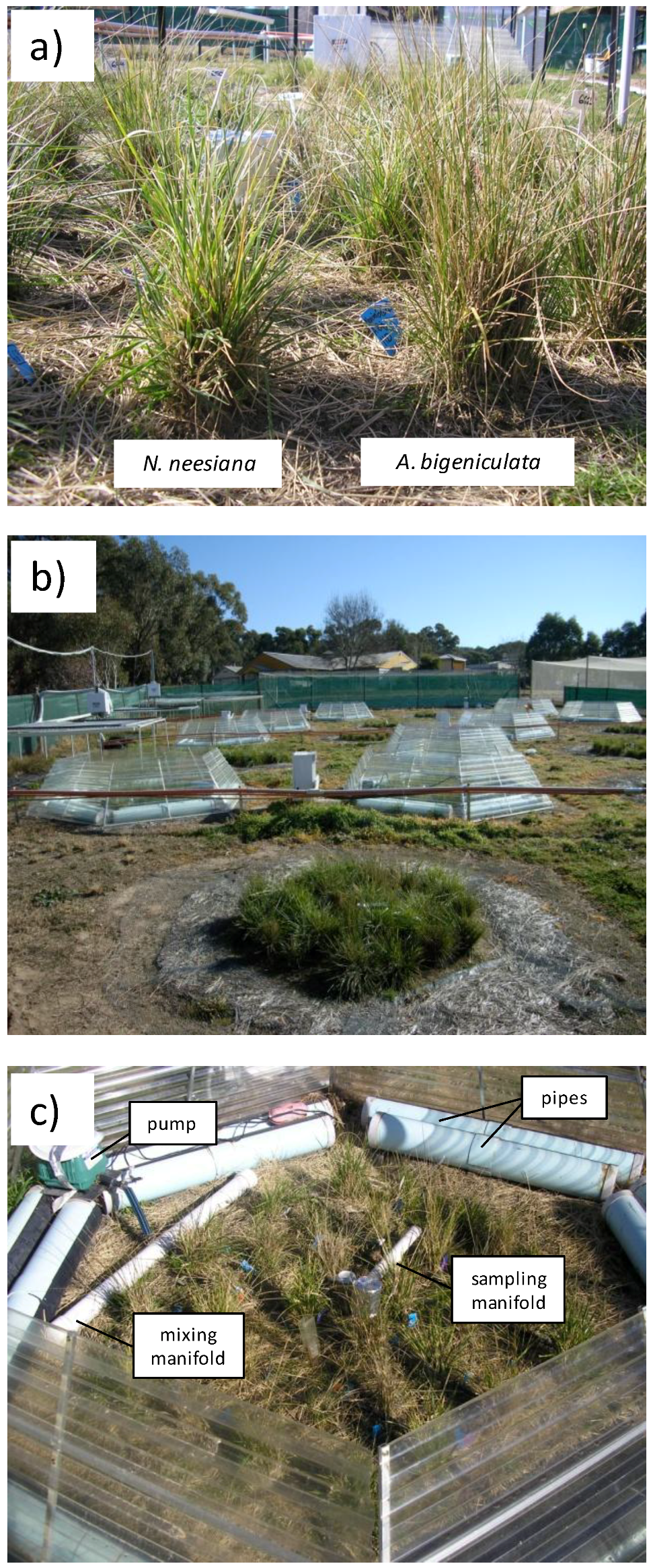
2.1. Study Species

Two C3 stipoid grasses were selected for comparison in the study: the Australian native Austrostipa bigeniculata (Hughes) S.W.L. Jacobs & J. Everett and the nonindigenous Nassella neesiana (Trin. & Rupr.) Barkworth (Chilean needle grass). Until recent taxonomic [49] and molecular data [50] supported the recognition of Austrostipa and Nassella, both species were members of the genus Stipa.

In Australia, Nassella neesiana is taxonomically difficult to distinguish from the similar species Nassella leucotricha (Trin. & Rupr.) R.W.Pohl (Texas needle grass). Until recently, all specimens collected from the study area, and the Australian Capital Territory (ACT), have been identified as N. neesiana. Recently, however, some have been re-identified as N. leucotricha sensu [51], primarily on the basis of length of the seed corona (>1.5 mm and <1.5 mm in N. leucotricha and N. neesiana respectively). However, in Australia and possibly in the Americas there is a lack of clarity regarding the morphological distinctiveness of these species, and taxonomic treatments contain some inconsistencies (c.f., [52,53,54]) that makes accurate identification difficult.

For example, some authors indicate that corona length overlaps in the two species (e.g., 0.7–2 mm vs. 0.5–1 mm; [52]). Examination of specimens from across Australia also suggests that coronal morphology exists as a continuum rather than as discrete groups, and indeed most morphological characters appear to overlap in both species [52]. Corona lengths ranged from 1.2–2.1 mm long in the four populations studied in this paper, suggesting possible affiliation with N. leucotricha sensu [52]; (but see [51] and [54]). Due to the poor current circumscription of the two species in Australia, and for consistency with the existing literature, in this paper were refer to all populations as Nassella neesiana sens. lat. However, we explicitly note that future work may identify all populations as N. leucotricha, or even reveal the presence of multiple taxonomic entities.

Austrostipa bigeniculata is a common to dominant species which grows widely across SE Australia, both in natural and derived grasslands [55,56,57]. Nassella neesiana was first recorded in Australia in 1934 and is now one of the nation’s worst weeds [54,58]. Infestations occur across SE Australia, especially in areas which receive more than 500 mm annual rainfall (Figure 1). In southern New South Wales (NSW), A. bigeniculata and N. neesiana have strongly overlapping ranges. Both species form tall (up to 1 m excluding flowering stems) perennial tussocks (Figure 2a). In contrast to A. bigeniculata, which mainly produce panicle seeds, N. neesiana also frequently produces cleiostogenes or “stem seeds” (chasmogamous seeds) at the nodes and bases of the stems [59], a feature that in other stipoid grasses increases fitness under stressful growing conditions, including heavy grazing and fire [59,60], soil moisture deficiencies [61] and other climatic cues.

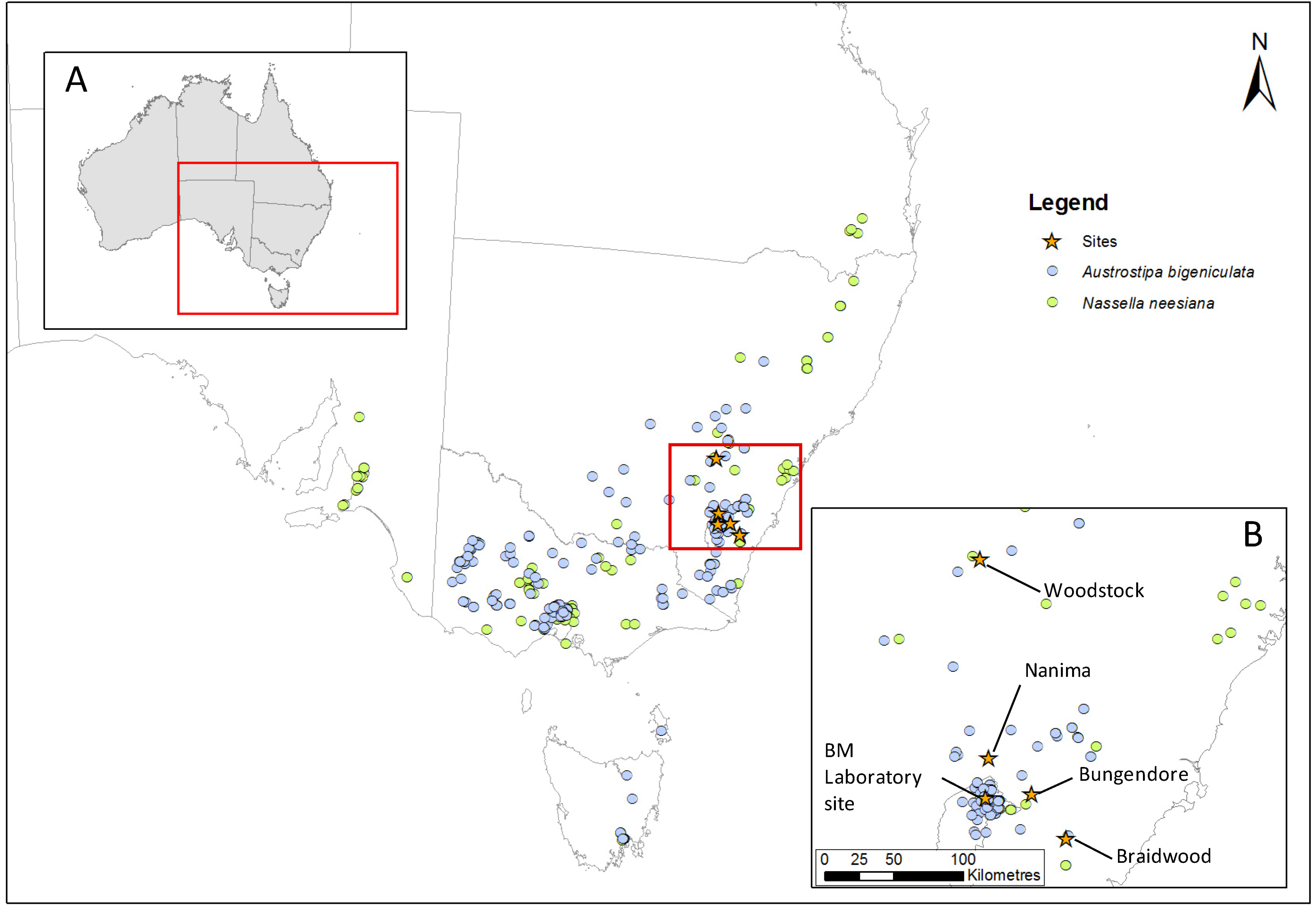
2.2. Site Selection and Description

Populations of A. bigeniculata and N. neesiana were collected from four sites along a 200 km transect in SE Australia (Figure 1): Braidwood (S 35.47°, E 149.79°), Bungendore (S 35.21°, E 149.48°), Nanima (S 35.01°, E 149.10°) and Woodstock (S 33.75°, E 148.84°). Temperature and potential evaporation (Table 1), and hence aridity and drought severity, increase with distance west along the transect, and vegetation changes considerably. We attempted to spread collection sites evenly along the transect, but were limited by the availability of N. neesiana, and so the two central sites (Bungendore and Nanima) had similar climatic characteristics (Table 1). The Braidwood site lay near the eastern range margin of both species, but the Woodstock site lay at the western margin of only N. neesiana—a few scattered populations of A. bigeniculata exist further to the west (Figure 1).

Figure 1. Schematic showing the study region (inset A) and herbarium specimen collection records for Austrostipa bigeniculata and Nassella neesiana across south-eastern Australia. The specific locations of the study sites along with the Black Mountain (BM) Laboratory site where glasshouse and field studies were performed are shown in inset B. Herbarium collection records were obtained from Australia’s Virtual Herbarium; see [62].

2.3. Specimen Collection and Propagation

Up to 50 A. bigeniculata and N. neesiana tussocks were collected from within a 1 ha collection area at each of the four study sites (Figure 1) between August and early December 2010. Randomly selected tussocks (at least 10 cm in diameter and 1 m apart) were removed from the ground and transported to the CSIRO Black Mountain Laboratory site (S 35.27°, E 149.11°; Figure 1) in moist sacks. Tussocks were then planted in 20 cm diameter pots in a 25 °C/15 °C day/night glasshouse and watered regularly for two weeks until they produced new leaf material. Pots contained standard high fertility potting mix and received one application of Scotts^® Osmocote^® Exact^® 3–4 month programmed release fertilizer (16% N as nitric and ammoniacal nitrogen, 9% P₂O₅, 12% K₂O, 2% MgO) at the time of planting to ensure adequate nutrient availability. Watering was performed as required. Plants established during late winter (August) were slower to respond than later collections and so tussocks tended to quickly converge in size.

Figure 2. The study species and experimental study site. (a) Ramets of Nassella neesiana and Austrostipa bigeniculata growing in a study plot. (b) The experimental site at Black Mountain, Australian Capital Territory (ACT), Australia, showing open-top chambers. The view is to the west. (c) Close-up of the inside of a chamber, showing pipes (containing water) arranged around the outside of the plot, along with the CO₂ injection pump, mixing manifold and sampling manifold.

Table 1. Climate data (1910–2009) for the four collection sites. Data were obtained from the SILO enhanced climatic data bank hosted by the Queensland Climate Change Centre of Excellence [63]. Tmax = maximum temperature; Tmin = minimum temperature; PET = potential evapotranspiration.

**Table 1.** Climate data (1910–2009) for the four collection sites. Data were obtained from the SILO enhanced climatic data bank hosted by the Queensland Climate Change Centre of Excellence [63]. Tmax = maximum temperature; Tmin = minimum temperature; PET = potential evapotranspiration.
		Collection site
		Braidwood	Bungendore	Nanima	Woodstock
Average Tmax (°C)
	Summer	24.9	26.9	27.4	30.0
	Autumn	19.1	19.7	20.1	22.3
	Winter	12.4	11.9	12.0	13.7
	Spring	18.8	19.4	19.7	22.0
	Annual	18.8	19.5	19.8	22.0
Average Tmin (°C)
	Summer	11.9	12.6	12.8	14.4
	Autumn	7.0	7.1	7.3	8.8
	Winter	1.3	1.1	1.4	2.9
	Spring	6.3	6.4	6.5	7.7
	Annual	6.6	6.8	7.0	8.5
Total precipitation (mm)
	Summer	208.7	166.8	152.6	177.2
	Autumn	192.4	151.5	147.2	140.5
	Winter	159.0	156.9	175.0	177.0
	Spring	186.8	184.0	183.8	182.8
	Annual	746.9	659.2	658.6	677.5
Total PET (mm)
	Summer	409.0	462.0	467.9	518.4
	Autumn	214.0	238.4	238.5	269.7
	Winter	120.2	124.4	121.9	132.0
	Spring	298.5	317.9	315.9	346.4
	Annual	1,041.7	1,142.7	1,144.2	1,266.5

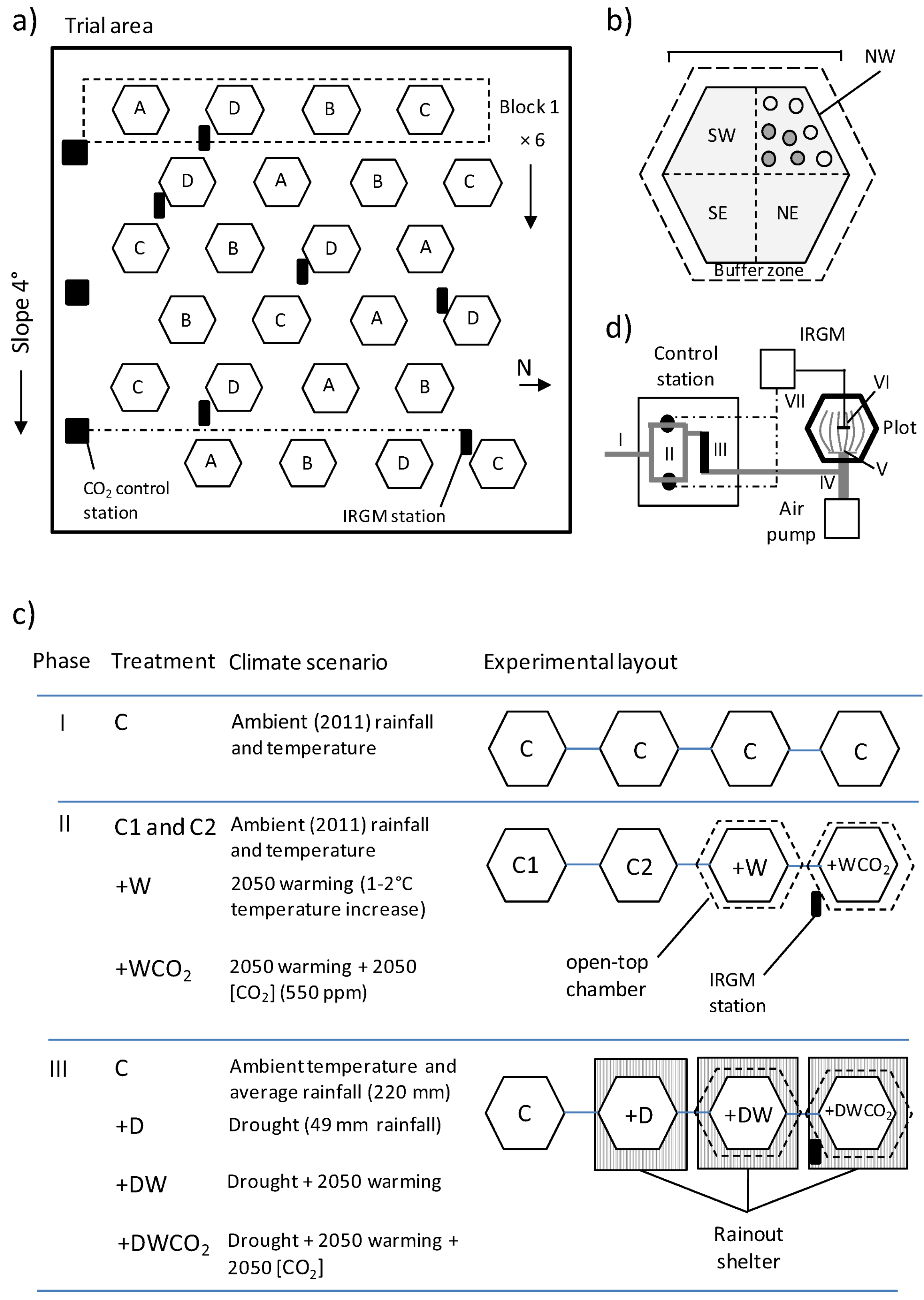
Once established, 24 healthy tussocks from each of eight populations (2 species × 4 collection sites) were selected, removed from pots, broken into four to seven equally sized ramets, and established in new 10 cm pots. All ramets taken from a single plant are henceforth referred to as a clone line, with each set of 24 clone lines representing a population. Ramets were allowed two weeks in the glasshouse to establish and were then moved outdoors for a further two weeks. Four well-established and (as much as possible) similarly-sized ramets were then selected from each clone line for use in the subsequent field trial. A total of 768 plants (4 ramets per clone line × 24 clone lines per population × 8 populations) were used in the trial.

2.4. Field Trial Design and Establishment

The field trial consisted of twenty-four 2.2 m² hexagon-shaped plots located within a 0.25 ha trial area at the CSIRO Black Mountain Laboratory site (Figure 3a). Plots were arranged into six blocks of four plots each, with blocks perpendicular to the aspect of the trial site (sloping 4° to the east; Figure 3a). This blocking arrangement captured potential site-level variation in soil water, soil nutrient level and shading associated with topographic position. The trial site was surrounded by a 2 m tall rabbit-proof fence covered with fine plastic mesh which reduced air flow and improved economy and control of CO₂ enrichment. Because of this design, and the proximity of buildings and trees to the site, we explicitly limited experimental inference to the low wind speeds (0–3 ms⁻¹ at 300 mm above ground) that occurred across the site during the study period.

The experiment was conducted in three discrete phases (Figure 3c), the first a common garden experiment, and the second and third involving climatic manipulation. Plots within blocks were allocated to one of four Phase III treatments (described below; labeled for convenience A–D in Figure 3a) corresponding to the climatic scenarios listed in Figure 3c. Each of the four treatments was replicated six times, once in each block (Figure 3a). The specific placement of ramets within plots ensured correct experimental design during all phases of the experiment.

Ramets were allocated to blocks and plots using a stratified random experimental structure in which one ramet from each of the 24 clone lines of each population occurred once in each Phase III treatment (Figure 3a,c; see below). Ramets from a given clone line (n = 4) were randomly allocated to different climate treatments (A–D) and then randomly to different blocks, thus reducing correlation between block and clone line. To balance the design, each plot contained four plants (one ramet from each of four randomly selected clone lines) from each population, for a total of 32 experimental plants. Within each plot, the 32 plants were arranged in a stratified random manner to reduce any effect of plot location on growth and reproduction. Plots were divided into four quadrants of equal size (NW, NE, SE and SW), each of which contained eight plants—a single ramet from each of eight populations (Figure 3b). Each plant was then randomly allocated to one of eight positions within the quadrant: half being along the edge of the quadrant and half on the inside (Figure 3b). This design was maximally efficient given the objectives and structure of the experiment and ensured that any positional and neighbor effects were randomly distributed with respect to species, population, and clone line.

Ramets were planted into plots during December and January 2011 and loosely packed with soil up to the base of the tussock crowns. Plants were watered until established (producing new green leaf material) and dead individuals were replaced with genetically identical ramets within 2–3 weeks. Soil in the plots consisted of a medium to high fertility sandy loam (Colwell P > 50 mg kg⁻¹; total N > 0.1%; total C = 1.2%–1.9%; and adequate K, Mg and Na), low salinity (electrical conductivity = 40–72 μS cm⁻¹), and low to moderate acidity (calcium chloride [CaCl₂] pH = 4.9–6.3). Sulphur levels were at or just below levels associated with adequate pasture availability (2.5–8.6 mg kg⁻¹).

Figure 3. Design and layout of the field experiment. (a) Layout of the study site. Each block (n = 6 total) contained four plots, each of which was assigned to one of four climate treatments in Phase III of the experiment (C, +D, +DW and +DWCO₂; labeled A–D) as defined in (c). (b) Layout of a study plot (n = 24 total). Hexagon-shaped plots (2.2 m²) were divided into four equal-sized quadrants (NW, NE, SE and SW), each of which contained eight plants—four inside (grey circles) and four edge (white circles). (c) Treatment structure, experimental layout and simulated climate scenarios during Phases I, II and III of the experiment. Note that the four climate treatments were randomly allocated to plots within each block. (d) Basic design of the CO₂ enrichment system. A line of pure CO₂ (I) is supplied to each CO₂-enriched chamber via a CO₂ control station [shown in (a)], where it is split into two lines, the flow of each being controlled by a solenoid valve (II). Both CO₂ lines then merge, pass through a flow meter (III), and enter a main air line (IV) which is supplied by a 60 L min⁻¹ air pump. The air and pure CO₂ then mix in a mixing manifold (V) and enter the plot via a series of porous CO₂ injection tubes. The CO₂ concentration is sampled by an infra-red gas monitor (IRGM) via a sampling manifold placed in the center of the plot (VI); the IRGM controls the solenoids via relays (VII) with different set-points for each of the solenoids (here 550 ppm and 575 ppm).

2.5. Field Trial Treatments and Climate Scenarios

The experiment proceeded in three phases (Figure 3c), each designed to test a different set of questions relevant to plant adaptation under climate change. During Phase I (February to April 2011) all plants were grown in a common garden experiment under ambient climatic conditions. This allowed determination of population-level quantitative variation and broad sense heritability [64,65] of growth variables without confounding by climate treatment effects (Figure 3c). During this period, total precipitation (161 mm) was just above the long term (1910–2009) Canberra average (145 mm). Observed mean maximum and minimum ambient screen temperatures were close to the 1980–1999 average (23.1 °C vs. 24.1 °C and 10.7 °C vs. 10.2 °C respectively). This timeframe is used for comparison with projected climate regimes (see [48]).

In Phase II (late April to June 2011) large open-top chambers (see [66]) were placed over two of the four plots in each block, one chamber of which received CO₂ enrichment to 550 parts per million by volume (ppm). Chambers raised atmospheric temperatures by 1–2 °C, thus simulating approximate year 2050 warming [48], while 550 ppm [CO₂] was adopted as a plausible scenario for 2050. Each block therefore contained two control plots with an ambient (2011) climate regime (C1 and C2) and a single plot containing 2050 warming (+W treatment) and 2050 warming + [CO₂] (+WCO₂). Specific treatment details are provided in Figure 3c. The objective of Phase II was to quantify the effects of future atmospheric warming and CO₂ enrichment on plant populations under non-drought conditions during winter, when water availability is usually high. During this phase rainfall was below average (22 mm vs. 89 mm) but plants did not visibly show moisture stress. Maximum ambient temperatures were near average (14.6 °C vs. 14.2 °C) but night minima were below normal (0.6 °C vs. 2.6 °C).

During Phase III (July to early November 2011) we imposed drought on +W and +WCO₂ treatments and one of the control replicates (C2), resulting in four new treatments: (1) control (C), (2) drought (+D), (3) drought + warming (+DW), and (4) drought +warming + elevated [CO₂] (+DWCO₂; Figure 3c). Control plots received 221 mm of rain during this period, equal to the Canberra average for the period, while drought-affected plots received 49 mm, only 22% of average. Drought rainfall was below the minimum (and first percentile) July to November 10 rainfall observed at Canberra and the four collection sites in the last century (65–85 mm), and so was clearly extreme. We note, however, that plot soil profiles also contained around 80 mm of plant available water in early July 2011, based on an estimated minimum plant available volumetric soil water content of 8% and a 70 cm root depth. Maximum ambient screen temperatures were above the 1980–1999 average (17.4 °C vs. 15.4 °C) but minimum temperatures were average (2.9 °C vs. 3.2 °C).

Atmospheric CO₂ enrichment was achieved using the simple, low-cost injection system previously reported in [66], but with a few modifications for larger-scale field experimentation (Figure 3d). CO₂ control is most precise during the day when photosynthetically active radiation (PAR) is highest but poorer on still, cold winter mornings and evenings when [CO₂] tends to exceed the target range of 550 ± 110 ppm. To conserve CO₂ we turned off the injection system outside of daylight hours and when wind speeds exceeded 10 ms⁻¹ (approximately 6% of total daylight hours). Drought was imposed on plots by covering them with rainout shelters (clear plastic tents) immediately prior to rainfall. Shelters were removed as soon as possible to reduce PAR interception (roughly 10%–20% of PAR during use) and were only in place for approximately 17% of total daylight hours.

2.6. Data Collection

To begin Phase I in February 2011 we cut all plants back to a height of 150 mm. This standardized plant size and allowed for accurate quantification of growth parameters but did not visibly reduce plant vigour. After 14 days we recorded leaf elongation, expressed as a daily rate (LER; mm day⁻¹), and the height to width ratio (HWR) of all tussocks, a measure of growth form in which higher score indicates a more upright stature. Width was determined by averaging two perpendicular measurements made across the tussock. In mid April 2011 we harvested all biomass above 150 mm, and determined the daily biomass accumulation rate (BAR; mg day⁻¹). We also determined the width, height (excluding stems), and the mid and basal diameters (compressed gently by hand) of all tussocks, and determined tussock volume (cm³). We also recorded the rate of flowering stem production (StemPR; stems plant⁻¹).

During Phase II, LER and BAR were again determined using the same methods as above; the amount of clipped material was small due to slow winter tussock growth and so impacts on plant growth were minimal. Phase III commenced in July 2011 with the watering of all plots to common soil water content (SWC) which allowed for the subsequent quantification of treatment effects on soil water. The drought regime was then imposed on C2, +W and +WCO₂ treatments, resulting in C, +D, +DW and +DWCO₂ treatments (Figure 3c). In August 2011 we again determined LER based on clipping a small section of tussock. We terminated the experiment on November 10 when some drought-stressed plants were approaching death and then commenced harvesting above-ground biomass (AGB) from tussocks. Due to time constraints, we only subsampled 24 ramets per population (25% of the total), evenly distributed across treatments. To ensure that no plants were killed by the procedure, we removed only a proportion of the basal area of each tussock. AGB was estimated for each plant by dividing the harvest weight (dried for 3 days at 70 °C) by the proportion of tussock basal area sampled of the total, assuming tussock symmetry. We also determined maximum length of flowering stems (MaxSL; cm), the flowering stem production rate (stems dm⁻² of tussock basal area), and the rate of floret production per inflorescence by counting floret numbers on up to ten inflorescences (if available) on each plant. Finally, we determined the total basal expansion (BasalE; mm) of each experimental plant over Phases II and III by comparing basal diameter in April and the final harvest date.

Plot temperatures were recorded in the center of each plot at 10 cm above the soil surface using Hobo^® Pendant UA-002-64 data loggers. To eliminate direct solar exposure, loggers were placed in small screens consisting of upturned pots covered in reflective silver tape. Data were recorded in two plots per treatment for 2–4 weeks during each month except in June when some loggers failed. SWC data were collected from the top 50–70 cm of the soil profile using neutron access tubes and a CPN Corporation Hydroprobe^® (Martinez, Ca). Volumetric SWC was calculated using the calibration equation:

SWC (% vol) = 2.0 × 10⁻⁷x² − 1.5 × 10⁻⁴x + 1.82

where x = the neutron probe reading, which was determined by comparing the SWC of soil core sections with probe readings taken at the time of removal. For a more detailed description of the methodology see [40].

2.7. Data Analyses

Growth and reproduction data were analyzed using general linear mixed model (LMM) analysis with model structure dependent on the experimental phase. Phase I models contained species (A. bigeniculata vs. N. neesiana), collection site (Braidwood, Bungendore, Nanima and Woodstock), the species × site two-way interaction term, planting (original vs. replacement), plot quadrant (Quad: NW, NE, SW and SE), quadrant position (Qpos: inside vs. edge) and Quad × Qpos, Quad × species, Qpos × species and Quad × Qpos × species interaction terms as fixed predictors (Table 2). Block (n = 6), plot within block (n = 4) and clone line within population (n = 24) were included as random predictor variables. Since data were missing for some variables block, Quad × Qpos × species and planting terms were removed from some models to ensure model convergence. Models and model degrees of freedom were estimated using REML and Satterthwaite methods respectively. We also determined estimated clone line means for each population and site and tested for differences among means using Tukey-Kramer—adjusted post-hoc means tests. Data were transformed where required to improve data conformity with model assumptions.

For one variable, April flowering stem production, data were highly skewed with many ramets producing no stems. Here, no transformation was entirely appropriate and so the data were analysed using generalized linear model analysis with stem count modeled as a Poisson distribution with log link and species, site, species × site, planting, Quad, and Qpos as predictor variables. Data were analysed using SAS Proc Mixed and Proc Genmod version 9.1 (SAS Institute Inc., Cary, NC, USA). Broad sense heritability (H²) of clonal lines was estimated for LER and BAR as H² = V_G/V_P where V_G is the genetic variance among clone lines and V_P is the total phenotypic variance [65,67]. Broad sense heritability represents an upper limit estimate of narrow sense heritability, estimates of which are based only on additive genetic variance. Variance estimates were obtained using SAS Proc Varcomp version 9.1 (SAS Institute Inc., Cary, NC, USA).

Linear mixed models for Phase II variables and LER in August contained the same terms as above but also climate treatment (Treat) (i.e., C1, C2, +W and +WCO₂ or C, +D, +DW and +DWCO₂) and associated two- and three-way interaction terms between Treat, species and site. We also included two-, three- and four-way interaction terms between Treat, Quad, Qpos and species, but to reduce model complexity we excluded higher order interaction terms between Quad, Qpos, species and site. As before, block, plot within block and clone line within population terms were included as random factors. Except for LER in August, Phase III data (Table 3) were collected by sampling a restricted set of plants and so were analysed using more simple models which excluded higher-order interactions involving the spatial terms Quad and Qpos (except the Treat × Qpos term), all of which were non-significant in Phase II models. Block and plot within block terms were included as random variables but clone line within population was excluded. We again compared predicted treatment × species (interaction) means for each variable, and where significant, species × site means, using Tukey-Kramer—adjusted post-hoc means tests. Data were analysed using SAS Proc Mixed version 9.1 (SAS Institute Inc., Cary, NC, USA).

Table 2. Results of linear mixed model analysis of trait data collected during Phase I of the experiment. Data in columns adjacent to fixed variables are F and associated p values (*** = p < 0.001; ** = p < 0.01; * = p < 0.05, ns = p ≥ 0.05); for random variables Z and p are provided. Estimated population means sharing the same letter did not differ at the 0.05 significance level.

**Table 2.** Results of linear mixed model analysis of trait data collected during Phase I of the experiment. Data in columns adjacent to fixed variables are F and associated p values (*** = p < 0.001; ** = p < 0.01; * = p < 0.05, ns = p ≥ 0.05); for random variables Z and p are provided. Estimated population means sharing the same letter did not differ at the 0.05 significance level.
			Dependent variable
			Leaf elongation rate (LER)		Height to width ratio (HWR)		Tussock width (Wid)		Tussock volume (Vol)		Height to width ratio (HWR)		Biomass accumulation rate (BAR)
Experimental phase measured			I		I		I		I		I		I
Month			February		February		February		April		April		Feb-April
Units			mm day⁻¹		none		mm		cm³		none		mg day⁻¹
Transformation			sqrt(×)		ln(×)		sqrt(×)		sqrt(×)		ln(×)		sqrt(×)
Model fixed effects (F, p)
	Species		52.2	***	831.2	***	540.3	***	399.9	***	719.1	***	18.5	***
	Site		129.8	***	82.1	***	49.7	***	35.7	***	31.8	***	57.0	***
	Species × Site		115.2	***	30.3	***	6.3	***	3.9	*	4.4	**	28.0	***
	Planting		68.5	***	2.8	ns	58.0	***	75.1	***	-		103.2	***
	Quadrant (Quad)		5.4	**	2.8	*	2.3	ns	0.1	ns	1.4	ns	5.6	***
	Quadrant Position (Qpos)		1.4	ns	25.1	***	18.1	***	50.4	***	78.5	***	1.1	ns
	Quad × Qpos		1.3	ns	3.1	*	1.5	ns	1.6	ns	3.5	*	0.8	ns
	Quad × Species		1.1	ns	1.4	ns	2.0	ns	2.8	*	0.9	ns	3.6	*
	Species × Qpos		2.0	ns	0.5	ns	0.0	ns	2.7	ns	2.1	ns	0.1	ns
	Quad × Species × Qpos		0.3	ns	0.7	ns	0.8	ns	0.5	ns	-		0.1	ns
Random effect (Z, p)
	Clone line		2.8	**	3.7	***	2.1	*	3.0	**	0.1	ns	4.7	***
	Block		1.4	ns	0.4	ns	1.2	ns	-		0.8	ns	1.2	ns
	Plot (Block)		1.2	ns	1.5	ns	1.6	ns	2.1	*	0.2	ns	2.4	**
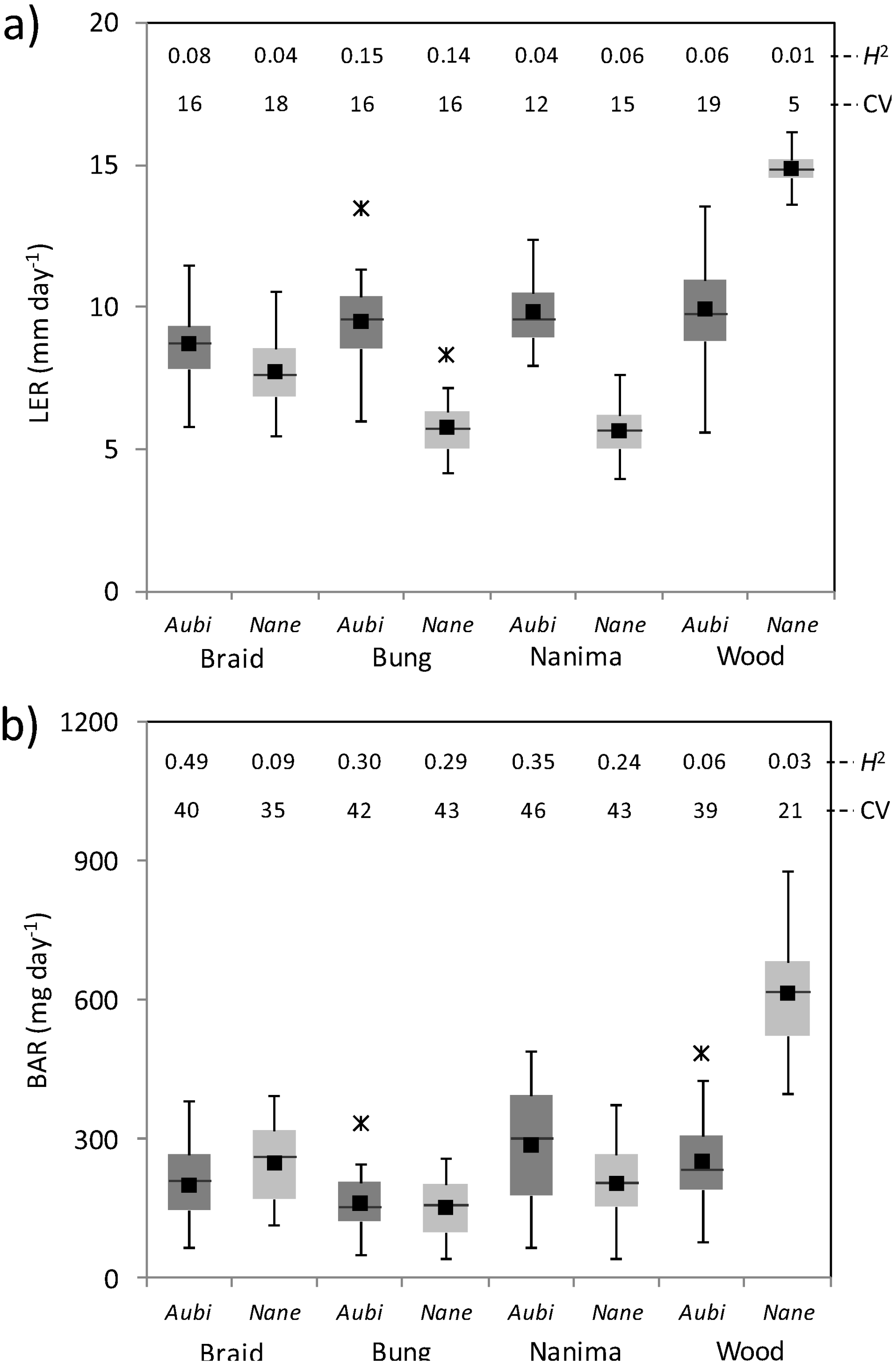
Estimated population means
	A. bigeniculata	Braidwood	2.94	cd	0.00	cd	17.3	bc	17.6	c	−0.12	c	13.8	bc
		Bungendore	3.08	bc	0.26	a	15.8	d	13.9	d	0.07	a	12.5	c
		Nanima	3.14	b	0.07	bc	17.2	c	18.2	c	−0.12	bc	16.4	b
		Woodstock	3.13	bc	0.15	ab	16.8	c	16.0	cd	−0.03	b	16.1	b
	N. neesiana	Braidwood	2.76	d	−0.50	f	20.4	a	27.8	a	−0.48	e	15.9	b
		Bungendore	2.40	e	−0.32	e	18.0	b	21.9	b	−0.39	d	12.0	c
		Nanima	2.38	e	−0.61	f	19.7	a	28.4	a	−0.53	e	13.8	bc
		Woodstock	3.86	a	−0.07	d	20.4	a	22.5	b	−0.35	d	24.6	a

Table 3. Results of linear mixed model analysis of trait data collected during Phases II and III of the experiment. Climate treatment acronyms are provided in Figure 3. Columns adjacent to fixed variables contain F and associated p values (*** = p < 0.001; ** = p < 0.01; * = p < 0.05, ns = p ≥ 0.05); for random variables Z and p are provided. Estimated means sharing the same letter did not differ at the 0.05 significance level. Only a restricted set of interactions involving quadrant and quadrant position are included; all others were not significant at the 0.05 significance level. Full model details are provided in the text. For species, Aubi = Austrostipa bigeniculata and Nane = Nassella neesiana.

**Table 3.** Results of linear mixed model analysis of trait data collected during Phases II and III of the experiment. Climate treatment acronyms are provided in Figure 3. Columns adjacent to fixed variables contain F and associated p values (*** = p < 0.001; ** = p < 0.01; * = p < 0.05, ns = p ≥ 0.05); for random variables Z and p are provided. Estimated means sharing the same letter did not differ at the 0.05 significance level. Only a restricted set of interactions involving quadrant and quadrant position are included; all others were not significant at the 0.05 significance level. Full model details are provided in the text. For species, Aubi = Austrostipa bigeniculata and Nane = Nassella neesiana.
					Dependent Variable
					Leaf elongation rate (LER)				Biomass accumulation rate (BAR)					Leaf elongation rate (LER)				Basal diameter (Basal D)
Experimental phase measured					II				II					III				III
Month					June				June					August				November
Units					mm day⁻¹				mg day⁻¹					mm day⁻¹				mm
Transformation					none				ln(×)					none				none
Model fixed effects (F,p)
	Species				60.7		***		65.1		***			166.1		***		155.5		***
	Site				44.2		***		23.1		***			15.4		***		10.8		***
	Species × Site				31.2		***		10.5		***			36.8		***		0.7		ns
	Climate treatment (Treat)				3.2		ns		2.4		ns			10.6		***		1.3		ns
	Treat × Species				6.5		***		5.2		**			2.9		*		1.3		ns
	Treat × Site				1.8		ns		0.6		ns			1.9		ns		0.9		ns
	Treat × Species x Site				0.9		ns		0.6		ns			0.9		ns		0.5		ns
	Planting				31.3		***		99.4		***			37.7		***		2.2		ns
	Quadrant (Quad)				1.4		ns		0.9		ns			1.8		ns		1.0		ns
	Quadrant position (Qpos)				0.3		ns		1.0		ns			15.9		***		24.9		***
	Treat × Quad				2.0		*		0.8		ns			0.3		ns		-
	Treat × Qpos				4.0		**		3.5		*			4.0		*		0.5		ns
Random effects (Z, p)
	Clone line				1.6		ns		2.7		**			3.8		***		-
	Block				1.4		ns		1.3		ns			1.3		ns		0.1		ns
	Plot(Block)				2.3		*		2.2		*			2.1		*		1.0		ns
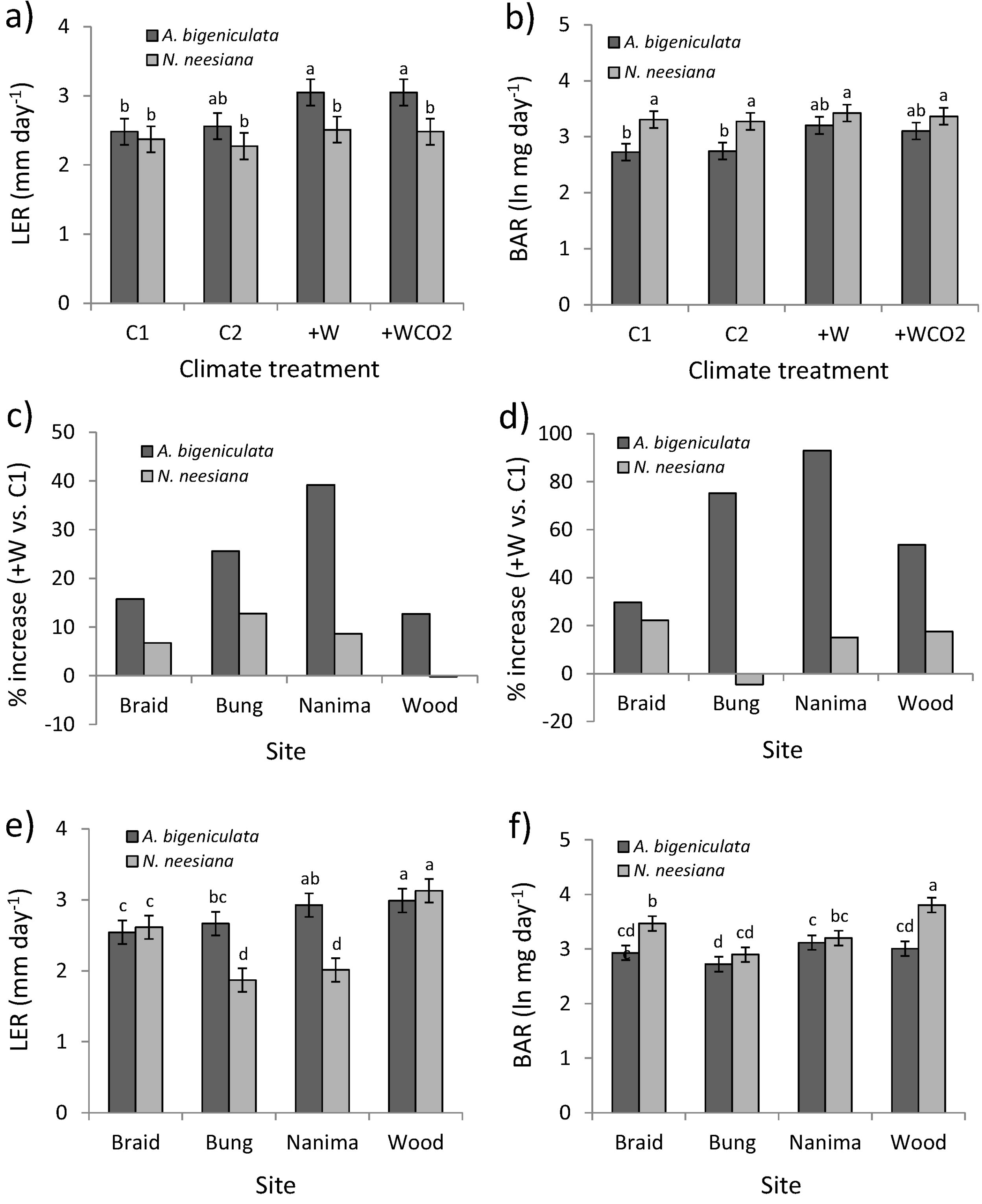
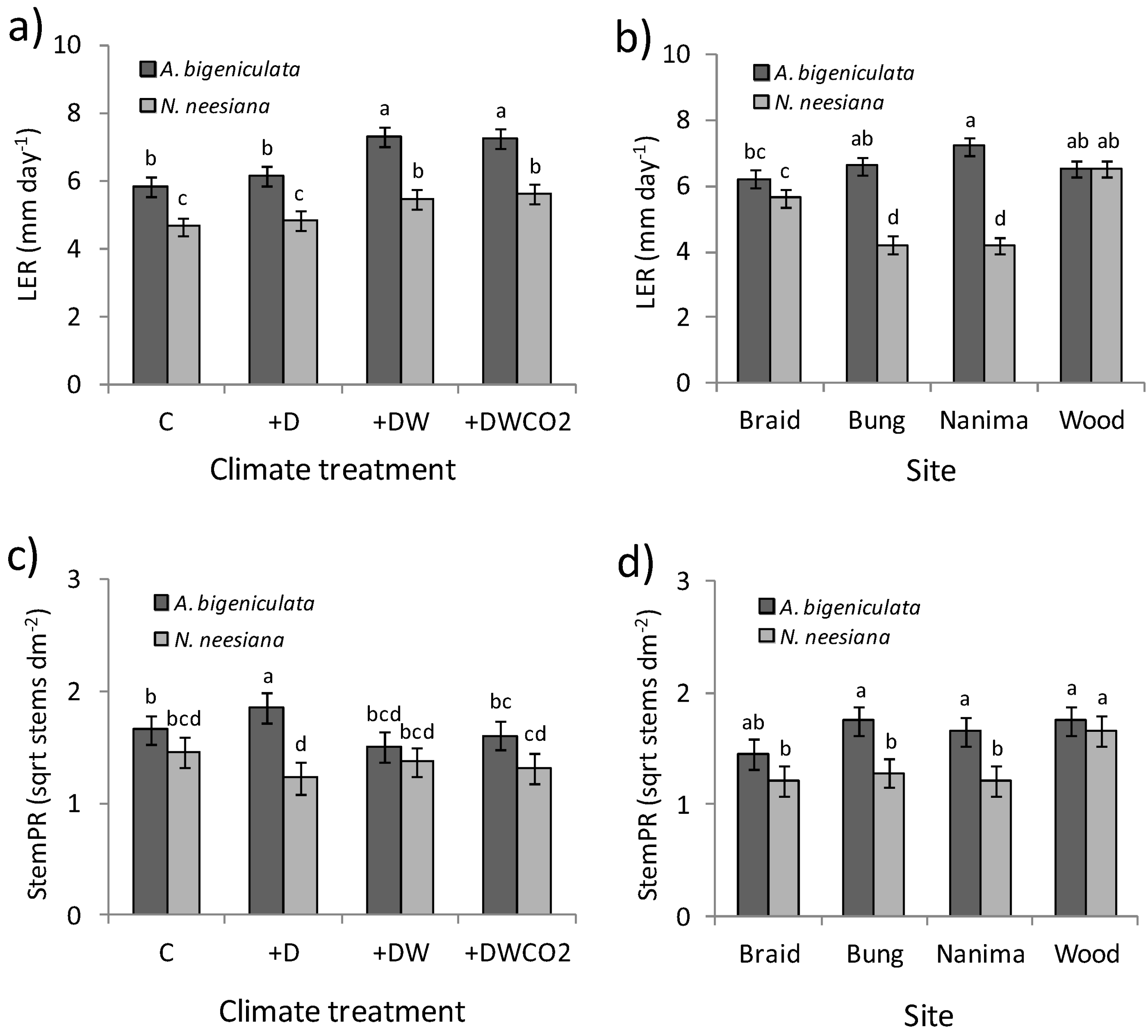
Estimated species x treatment means
	Phase II	Phase III	Species
	C1	C	Aubi		2.48		bc		2.73		b			5.87		b		57.1		b
	C2	+D	Aubi		2.56		b		2.74		b			6.15		b		47.2		b
	+W	+DW	Aubi		3.05		a		3.20		ab			7.33		a		59.4		b
	+WCO₂	+DWCO₂	Aubi		3.05		a		3.10		ab			7.25		a		55.5		b
	C1	C	Nane		2.37		bc		3.31		a			4.67		c		84.1		a
	C2	+D	Nane		2.27		c		3.27		a			4.84		c		84.3		a
	+W	+DW	Nane		2.51		bc		3.42		a			5.49		b		86.5		a
	+WCO₂	+DWCO₂	Nane		2.48		bc		3.37		a			5.62		b		92.3		a
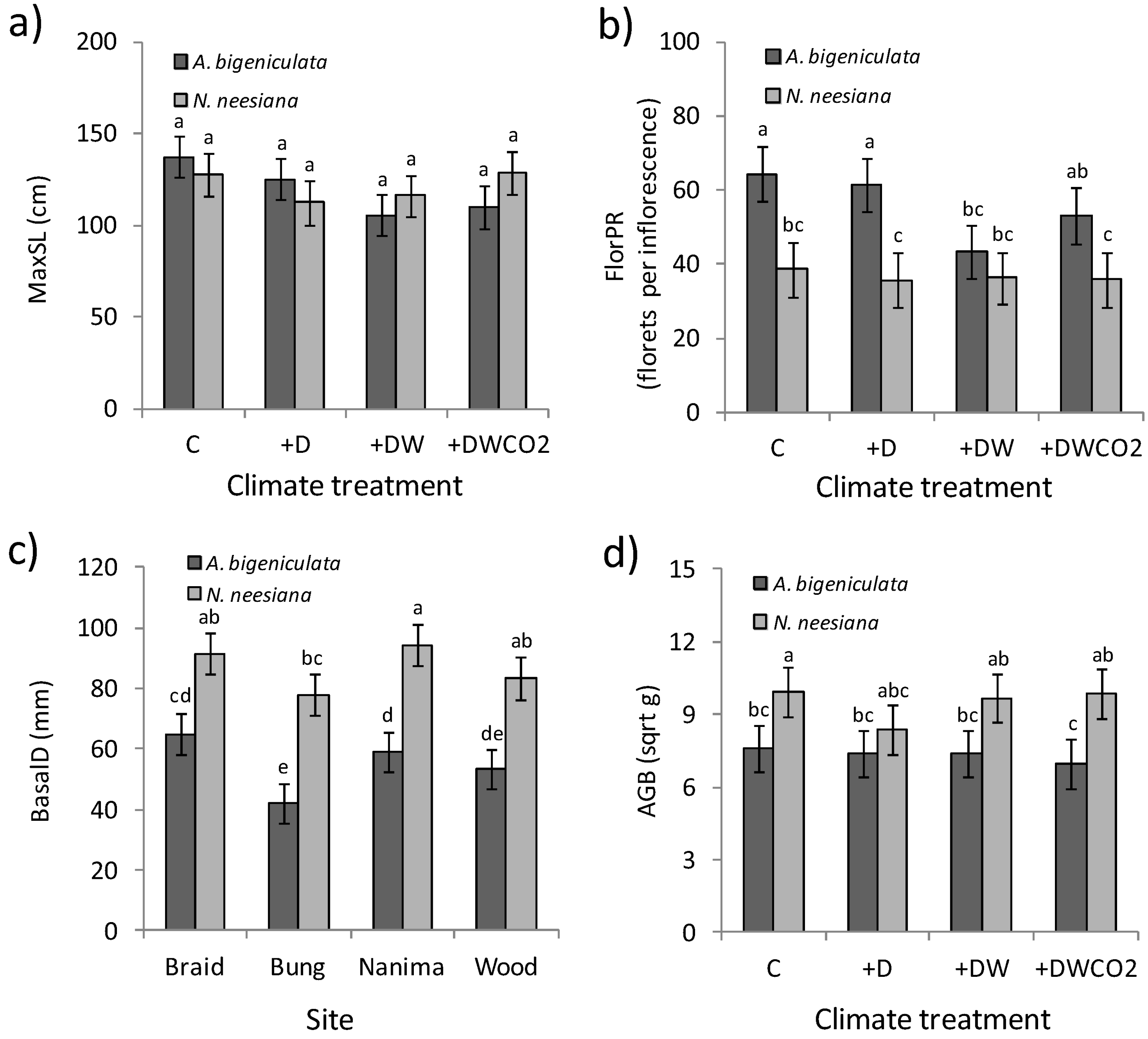
				Dependent Variable
				Basal expansion (BasalE)				Maximum stem length (MaxSL)				Above ground biomass (AGB)			Stem Prod Rate (StemPR)				Floret production rate (FlorPR)
Experimental phase measured				III				III				III			III				III
Month				November				November				November			November				November
Units				mm				cm				g			stems dm⁻²				florets infl⁻¹
Transformation				none				none				sqrt(×)			sqrt(×)				none
Model fixed effects (F,P)
	Species			11.8		***		0.2		ns		35.2	***		39.0		***		53.6		***
	Site			2.5		ns		2.1		ns		7.3	***		10.3		***		0.9		ns
	Species × Site			1.4		ns		1.8		ns		2.8	*		3.1		*		2.0		ns
	Climate treatment (Treat)			1.1		ns		1.9		ns		0.6	ns		1.0		ns		2.9		ns
	Treat × Species			0.6		ns		3.9		*		1.3	ns		4.8		**		3.0		*
	Treat × Site			0.9		ns		0.1		ns		0.6	ns		1.6		ns		0.8		ns
	Treat × Species x Site			0.5		ns		0.3		ns		0.5	ns		0.8		ns		0.8		ns
	Planting			1.6		ns		0.3		ns		2.4	ns		0.0		ns		1.0		ns
	Quadrant (Quad)			0.1		ns		0.8		ns		0.3	ns		0.5		ns		0.3		ns
	Quadrant position (Qpos)			2.0		ns		6.5		*		27.2	***		0.4		ns		12.3		***
	Treat × Quad			-				-				-			-				-
	Treat × Qpos			1.3		ns		1.3		ns		0.0	ns		0.8		ns		0.8		ns
Random effects (Z, P)
	Clone line			-				-				-			-				-
	Block			0.6		ns		0.2		ns		0.3	ns		0.5		ns		-
	Plot(Block)			0.6		ns		1.8		*		1.3	ns		0.8		ns		0.8		ns
Estimated species x treatment means
	Phase II	Phase III	Species
	C1	C	Aubi	4.1		ab		137.4		a		7.6	bc		1.66		b		64.4		a
	C2	+D	Aubi	1.9		ab		125.2		a		7.4	bc		1.85		a		61.6		a
	+W	+DW	Aubi	1.8		b		105.6		a		7.4	bc		1.50		bcd		43.3		bc
	+WCO₂	+DWCO₂	Aubi	6.3		ab		110.1		a		7.0	c		1.61		bc		53.0		ab
	C1	C	Nane	7.6		ab		128.1		a		9.9	a		1.45		bcd		38.8		bc
	C2	+D	Nane	11.2		ab		112.5		a		8.3	abc		1.23		d		35.8		c
	+W	+DW	Nane	12.4		a		116.3		a		9.7	ab		1.37		bcd		36.3		bc
	+WCO₂	+DWCO₂	Nane	18.7		a		129.0		a		9.8	ab		1.32		cd		36.0		c

We also tested for differences in mean volumetric soil water content (SWC%) and change in soil water content (∆SWC) across a range of time intervals during the Phase III of the experiment. We determined SWC for all plots at depths of 10 cm, 20 to 40 cm and 50–70 cm on 7 July, 1 August, 23 August, 6 October and 10 November 2011, and determined ∆SWC for the intervals 7 July to 1 August, 23 August to 6 October, and 6 October to 10 November. Variables were analyzed using linear mixed model analysis with climate treatment and block as fixed predictor variables; predicted treatment means were tested using Tukey-Kramer—adjusted post-hoc means tests. All LMM analyses were performed using SAS Proc Mixed version 9.1.

3. Results

3.1. Temperature and [CO₂]

Warming generated by the open-top chambers was broadly in line with previous observations [66]. Daytime (06:00–17:30) warming was generally around 1–2 °C in all months except July when it ranged from 0–1 °C (Table 4). Daily maximum temperatures were generally elevated more than mean daily temperatures. At night (18:00–05:30) temperatures were usually 0.5–1.5 °C warmer inside chambers although extreme minima were as much as 2.2 °C higher (Table 4). Daytime mid-canopy atmospheric [CO₂] averaged 576 ppm across the six enriched chambers (range 541–612 ppm).

Table 4. Temperatures observed under different climate treatment regimes during the experiment. Actual temperatures are shown for ambient control plots (shaded) while deviations from the control are shown for treatments. Treatment acronyms are described in Figure 3. Tav = average temperature, Tmax = average daytime maximum, Temax = extreme (highest) daytime maximum, Tmin = average night minimum, Temin = extreme (lowest) night minimum.

**Table 4.** Temperatures observed under different climate treatment regimes during the experiment. Actual temperatures are shown for ambient control plots (shaded) while deviations from the control are shown for treatments. Treatment acronyms are described in Figure 3. Tav = average temperature, Tmax = average daytime maximum, Temax = extreme (highest) daytime maximum, Tmin = average night minimum, Temin = extreme (lowest) night minimum.
	Climate Treatment	Day			Night
Month	Climate Treatment	Tav	Tmax	Temax	Tav	Tmin	Temin
May	Control	9.9	15.5	20.7	3.0	0.3	-3.1
	+W	+0.6	+1.6	+2.0	+0.9	+1.1	+1.1
	+WCO₂	+0.5	+1.0	+1.1	+1.1	+1.3	+1.3
July	Control	8.3	13.6	19.0	3.9	0.9	−2.5
	+D	0.0	0.0	-0.4	+0.1	+0.1	−0.2
	+DW	+0.5	+1.0	-0.1	+0.4	+0.5	+0.2
	+DWCO₂	+0.4	+0.6	-0.2	+0.4	+0.6	+0.8
August	Control	11.9	18.5	23.9	6.2	2.9	−0.9
	+D	+0.5	+0.9	+0.7	0.0	+0.1	+0.2
	+DW	+1.0	+2.0	+2.4	+0.6	+1.0	+1.6
	+DWCO₂	+1.1	+1.5	+2.2	+0.8	+1.3	+2.0
September	Control	15.3	21.9	29.0	7.9	4.1	−1.1
	+D	+0.9	+1.4	+1.6	+0.3	+0.4	+0.6
	+DW	+1.9	+3.1	+3.1	+0.8	+1.0	+1.1
	+DWCO₂	+1.5	+1.7	+1.0	+1.2	+1.6	+2.2
October	Control	20.7	29.2	37.1	11.7	8.6	1.8
	+D	+0.8	+0.8	+0.7	+0.3	0.0	−0.3
	+DW	+1.1	+1.9	+2.3	+0.7	+0.4	+0.4
	+DWCO₂	+1.1	+0.6	0.0	+0.8	+0.5	+0.8

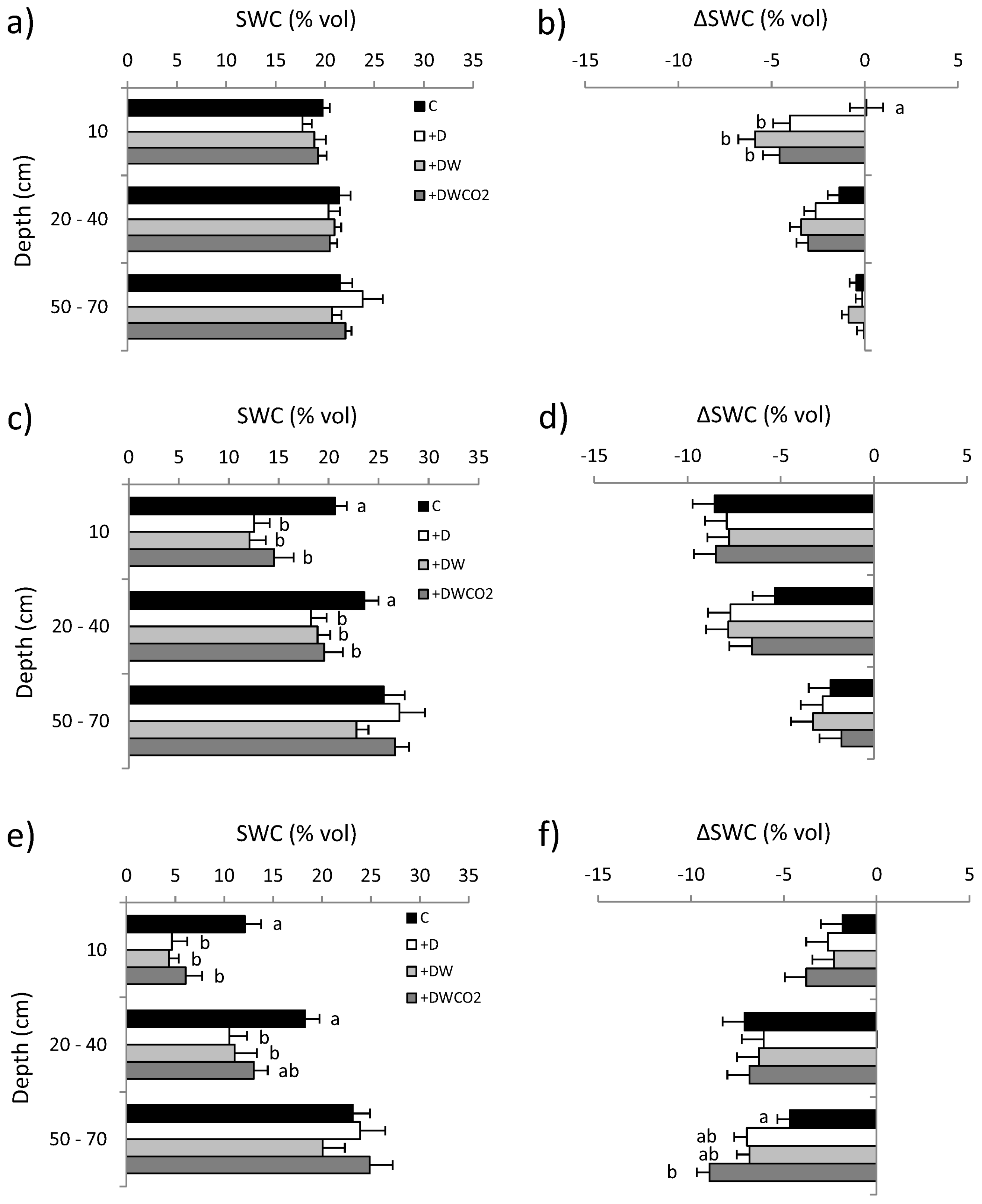
3.2. Soil Water Content

On 7 July 2011, at the start of Phase III of the experiment, no differences in SWC (p > 0.2) were evident anywhere in the soil profile (Figure 4a). Plant-available water reserves were adequate (Figure 4a) and plants showed no signs of moisture stress. After 25 days (7 July–1 August) SWC change (∆SWC) in the upper profile varied significantly across treatment regimes (F_3,15 = 8.03, p < 0.01), with SWC declining by close to 5% in all treatments except the control (Figure 4b). No significant differences between +D, +DW and +DWCO₂ treatments were observed. Soil water also declined in the mid profile (Figure 4b), but treatment-level differences were not significant (F_3,15 = 1.68, p = 0.21).

Figure 4. Volumetric soil water content (SWC, %) in experimental plots during winter and spring 2011. (a) SWC on 7July 2011 in the upper (10 cm), mid (20–40 cm) and lower (50–70 cm) soil profile. (b) Change in SWC over the period 7July to 1August 2011. (c) SWC on 23August 2011. (d) Change in SWC over the period 23August to 6October, 2011. (e) SWC on 6October 2011. (f) SWC change over the period 6October to 10November 2011. Data are estimated means based on six experimental plots ± one standard error. Within each depth and timeframe, means sharing the same letter are not significantly different at the p = 0.05 level; only those in which at least two means differed are shown.

By August 23 significant (p < 0.05) differences had emerged across treatments in the upper and mid soil profile, with SWC being up to 8% lower in drought-affected plots than in control plots (Figure 4c). Differences were more pronounced in the upper profile, and again, there was no evidence that warming or atmospheric CO₂ enrichment affected SWC (cf., +D vs. +DW and +DW vs. +DWCO₂) (Figure 4c). Between 23 August and 6 October, SWC declined greatly throughout the soil profile (Figure 4d), leading to extreme upper profile soil water deficiencies in all treatments except the control (Figure 4e). By this time, stress (e.g., leaf rolling) was observable in plants across +D, +DW and +DWCO₂ treatments. Over the next 34 days SWC declined rapidly in the mid and lower soil profile, but remained above 10% in control plots. Water loss was again unrelated to treatment except in the lower rhizosphere (F_3,15 = 6.87, p < 0.01) where loss was greatest in the +DWCO₂ treatment and least in the control (Figure 4f). By the end of the experiment most plants in non-control plots showed signs of either moderate or severe moisture stress.

3.3. Plant Growth and Reproduction

LMM analysis indicated that, under Phase I (ambient) common garden conditions, species (Nassella vs. Austrostipa), collection site and planting (original vs. replanted) were by far the strongest predictors of plant growth, reproduction and stature (Table 2). Although significant (p < 0.05) species × site interactions were present in all models, the width (Wid), volume (Vol) and stature (HWR) of tussocks were largely determined by species differences, with the overall larger size of N. neesiana indicating more rapid lateral growth and tussock expansion. With the exception of the Woodstock population (species × site interaction p < 0.05), N. neesiana tussocks were also more prostrate than those of A. bigeniculata (lower HWR; Table 2). N. neesiana produced many fewer flowering stems than A. bigeniculata (χ² = 151.7, p < 0.001) during April (average = 0.04 vs. 0.64 stems dm⁻²), although species differences did depend significantly, but less strongly, on site (species × site interaction χ² = 12.9, p < 0.01). Species differences in leaf elongation (LER) and biomass accumulation (BAR) depended more strongly on collection site (Table 2, Figure 5), with Woodstock N. neesiana exhibiting exceptionally rapid growth.

Replanted ramets tended to be smaller, to grow more slowly, and to have lower reproduction than original plants. Spatial (quadrant and quadrant position) predictors were also significant in some models (Table 2); in particular, plants growing on the inside of quadrants tended to be smaller and less prostrate than those located along the quadrant edge, and those in NE and NW quadrants grew more slowly than those in SW and SW quadrants. However, these effects tended to be much weaker than the species- and site-level differences previously described.

No clear clinal patterns were observed in any variable (Table 2) although leaf elongation rate in A. bigeniculata increased slightly with distance west of the collection site (Figure 5a). Variation in LER and BAR (Figure 5) was greater among N. neesiana populations, mainly reflecting the rapid growth of N. neesiana plants from Woodstock (Table 2; Figure 5a,b). Within-population (among clone line) variability (coefficient of variation of clone line means) in LER and BAR was generally similar in both species although the Woodstock N. neesiana population had reduced variation in both traits(Figure 5). Broad sense heritability (H²) was lower in LER than in BAR and tended to be lower in N. neesiana than A. bigeniculata. In N. neesiana H² of both variables was lower in the range-edge Braidwood and Woodstock populations than in the range-core Nanima and Bungendore populations (Figure 5), but in A. bigeniculata this pattern was only observed for BAR in the Woodstock population (Figure 5a).

Figure 5. Boxplots showing growth of A. bigeniculata and N. neesiana tussocks during Phase I of the experiment. (a) Leaf elongation rate (LER) in February 2011. (b) Biomass accumulation rate (BAR) during February–April 2011. Data are based on estimated means for each clone line (n = 24) within each of the eight plant populations (four A. bigeniculata and four N. neesiana populations). Numbers at the top of each panel are the broad sense heritability (H²) and the coefficient of variation (CV; expressed as a percentage of the mean) of the trait across clone lines (see methods). For species names, Aubi = Austrostipa bigeniculata and Nane = Nassella neesiana. For site names, Braid = Braidwood, Bung = Bungendore, Nanima = Nanima, and Wood = Woodstock (see Figure 1).

During Phase II species-level differences were again highly significant (p < 0.001; Table 3); overall A. bigeniculata exhibited more rapid leaf elongation (Figure 6a) but slower biomass accumulation (Figure 6b) than N. neesiana. However, differences depended on treatment (interaction p < 0.01; Table 3). For LER, species differences were only significant in +W and +WCO₂ treatments (Figure 6a), since increased leaf growth due to warming (i.e., +W treatment vs. C1 treatment) was much more pronounced in A. bigeniculata (12%–40%) than in N. neesiana (0%–13%; Figure 6c). Indeed, differences among treatments were significant in A. bigeniculata (p < 0.01) but not in N. neesiana (p = 0.52). For BAR, A. bigeniculata was more responsive to warming than N. neesiana, with treatment differences being significant only in A. bigeniculata (p < 0.01 vs. p = 0.77). Interspecific differences in BAR were greatest in control plots (C1 and C2; Figure 6b), due to the lack of response in N. neesiana to warming (Figure 6d); indeed, means of the two species in warmed treatments (+W and +WCO₂) did not differ (Figure 6b). Species differences also depended strongly on collection site (interaction p < 0.001; Table 3). Leaf elongation was more rapid in A. bigeniculata than N. neesiana collected from Bungendore and Nanima (Figure 6e), while biomass accumulation was greater for N. neesiana than A. bigeniculata populations collected from the Braidwood and Woodstock sites (Figure 6f). There was again a trend towards increased leaf growth in A. bigeniculata populations collected from drier, warmer sites (Figure 6e), and variation among populations (sites) was higher in N. neesiana for both LER and BAR (Figure 6e,f).

Figure 6. Leaf and biomass growth during Phase II of the experiment (June 2011). (a) Estimated leaf elongation rate (LER) (±1 SE) across climate treatments. (b) Estimated biomass accumulation (BAR) (±1 SE) across climate treatments. (c) Percentage increase in LER between warming (+W) and control (C1) treatments for each of the study populations. (d) Percentage increase (untransformed data) in BAR between warming (+W) and control (C1) for each of the study populations. (e) and (f) Estimated mean (±1 SE) LER and BAR across the study populations. Means sharing the same letter do not differ significantly at the 0.05 level. Climate treatment and site acronyms are as in Figure 3, Figure 5.

During Phase III of the experiment drought was imposed and soil water declined (Figure 4). Early in this period (August), rain exclusion had no impact on leaf elongation (LER) (c.f., C and +D climate treatments, Figure 7a), but for both species growth was greater in warmed (+DW and +DWCO₂) treatments than in the control. The increase in growth was greater in A. bigeniculata (23–25%) than in N. neesiana (18–20%), and while significant (p < 0.05), the associated treatment × species interaction term was weak relative to the main effects of species, site and climate treatment (Table 3). There was no evidence that CO₂ enrichment altered leaf elongation rate in either species (c.f., +DW vs. +DWCO₂ treatments; Figure 7a). The cline in LER across A. bigeniculata populations observed in June was weaker in August (Figure 7b), but differences among N. neesiana populations exhibited a similar pattern and there was again a much higher level of interpopulation variation than in A. bigeniculata (Figure 7b).

Figure 7. Growth of A. bigeniculata and N. neesiana during Phase III of the experiment. (a) Leaf elongation (LER) across climate treatments during August 2011. (b) LER across study populations during August 2011. (c) Stem production (StemPR) across climate treatments in November 2011. (d) StemPR across study populations in November 2011. Data are estimated means ± 1 standard error; means sharing the same letter do not differ significantly at the 0.05 level. Climate treatment and site acronyms are as in Figure 6.

By November 2011, following an extended period of extremely low soil water, significant treatment × species interactions were observed in three variables: stem production rate (StemPR), maximum flowering stem length (MaxSL), and floret production rate (FlorPR) (Table 3). There was a strong overall pattern towards higher stem production in A. bigeniculata across treatments (main species effect p < 0.001; Table 3), although a significant (p < 0.05) post-hoc adjusted species difference was evident only in only in the drought (+D) climate treatment (Figure 7c). Stem production in A. bigeniculata exceeded that of N. neesiana only in Bungendore and Nanima populations (Figure 7d), resulting in a significant (p < 0.05) species × site interaction term for this variable (Table 3).

The linear mixed model for MaxSL (Table 3) indicated that the two study species again responded differently to the range of climate treatments, albeit weakly (p < 0.05), with stem length influenced by the combination of drought and atmospheric warming only in A. bigeniculata. While A. bigeniculata treatment means differed only marginally (e.g., C vs. +DW mean difference p = 0.07; Figure 8a), overall differences among treatments were significant (p = 0.03), with stem length being ~20% lower in +DW and +DWCO₂ treatments compared with the control. A similar pattern was observed for floret production, which, in A. bigeniculata, was significant reduced in the +DW treatment compared with the control (Figure 8b). Interestingly, drought (+D treatment) appeared to have no direct influence on floret production (Figure 8b). There was little evidence that atmospheric CO₂ enrichment mitigated the effects of drought and heat stress observed in A. bigeniculata, with the possible exception of floret production (Figure 8b). In contrast to A. bigeniculata, N. neesiana did not differ significantly in stem length, stem production and floret production across any climate treatments (Figure 7c, Figure 8a,b; Table 3).

Figure 8. Reproduction and growth in A. bigeniculata and N. neesiana during Phase III of the experiment. (a) Maximum length of flowering stems (MaxSL) across climate treatments. (b) Floret production rate (FlorPR) across climate treatments. (c) Tussock basal diameter (BasalD) across study collection sites. (d) Above ground biomass (AGB) across climate treatments. Data are estimated means ± 1 standard error; means sharing the same letter do not differ significantly at the 0.05 level. In panel (a) estimated means differed at the 0.10 level (see text). Climate treatment and site acronyms are as in Figure 6.

Other variables related to plant size and biomass (BasalD, AGB) also exhibited strong interspecific differences (Table 3), with N. neesiana tussocks being 62% wider and having 32% more biomass than those of A. bigeniculata (Figure 8c,d). These species-level differences tended to be similar across sites (e.g., Figure 8c) and treatments (Figure 8d), consistent with the very strong main effect of species and weaker site × species and treatment × species effects in the associated linear mixed models (Table 3). Tussock expansion (BasalE) in N. neesiana during Phases II–III of the experiment was more than double that of A. bigeniculata (Table 3).

4. Discussion

4.1. Drought, Climate and Adaptation in A. bigeniculata and N. neesiana

Despite being closely related stipoid grasses, N. neesiana and A. bigeniculata responded differently to atmospheric warming and soil drought. The observed patterns of change, however, provide little or no support for the hypothesis (H1) that NIPS advantage should be highest under more favorable growing conditions. Indeed, our data indicate that the NIPS N. neesiana is, if anything, less affected by thermal and hydrological change than the native species A. bigeniculata. This pattern was especially evident in the responses of leaf elongation and biomass accumulation to warming during autumn and early winter, which show that amelioration of cold temperatures most advantaged A. bigeniculata over N. neesiana. Indeed, species differences for these variables depended entirely on the presence or absence of atmospheric warming (Figure 6a,b).

There was also no evidence that N. neesiana growth and reproduction disproportionately declined under stressful (drought) conditions (c.f., [27]). Indeed, reproductive fitness (floret production) declined more in plots subjected to warming and drying (+DW treatment, Figure 8b) in A. bigeniculata than in N. neesiana, and similar trends occurred in maximum flowering stem length (Figure 8a) and (to a lesser extent) flowering stem production (Figure 7b). Whether these patterns reflect greater plasticity in resource allocation or phenology of N. neesiana under drought conditions (e.g., [68]) remains to be determined, but we did observe that the shift towards earlier flowering in drought treatments (+D, +DW and +DWCO₂) was greater in N. neesiana (6.8 days) than A. bigeniculata (3.8 days; data in preparation). This may have helped generate the drought-related NIPS advantage in reproduction observed in N neesiana during the experiment. On the other hand, the much greater rate of autumn (April) flowering in A. bigeniculata is suggestive of a more facultative seed production in response to water availability, and indeed in southern NSW flowering in N. neesiana tends to be more tightly restricted to the spring and early summer. It must be remembered, however, that N. neesiana also produces cleistogamous stem and basal seeds, which may provide additional reproductive flexibility that supplements variation in timing and magnitude of panicle seed production [59]. This might mitigate any fitness consequences associated with the autumn flowering differential observed during our study.

However, while A. bigeniculata exhibited larger responses to warming and drought, N. neesiana still outperformed A. bigeniculata overall. By the end of the common garden experiment, N. neesiana tussocks were significantly larger than those of A. bigeniculata, and these differences increased through winter and spring. By the end of the experiment, mean basal diameter of N. neesiana tussocks was ~60% larger than that of A. bigeniculata, which alone doubled their relative potential reproductive fitness, at least in terms of total plant floret production. These differences probably arose primarily when water availability was adequate for growth, since in both species severe water stress developed only towards the end of the experiment. However, enhanced drought tolerance or water use efficiency [69] may also have contributed to the observed size differences.

The overall NIPS advantage observed in N. neesiana is not entirely unexpected since its invasiveness is thought to stem, as in many other weedy species [26,70], from its rapid growth rate and competitive ability [54]. The rapid biomass accumulation and prostrate growth habit observed in our study support the view that N. neesiana is highly competitive for light and other resources in grasslands, perhaps in an asymmetric manner in which initial differences in resource capture rates arising from size inequality are magnified by positive feedback between growth and resource acquisition [71,72,73]. It is also possible that other factors such as the presence of disease in sympatric native grass populations (for example in Austrostipa; [74]) and release from specialist pathogens (the enemy release hypothesis; [75]) may in part explain the competitive superiority of N. neesiana in mixed species stands and its ability to displace even dominant native species [58].

Collectively, our data suggest that overall NIPS advantage in N. neesiana is associated with rapid tussock expansion and increased plant basal area when soil water is available for growth. Since flowering stem production is related to overall plant size, this increases total reproductive potential if water availability reaches critical levels during spring drought. It appears that winter warming is likely to reduce this NIPS advantage but increasingly severe spring droughts may increase it. However, it is important to point out several caveats to this conclusion. First, we only simulated brief, acute drought, and, during spring, warming was unavoidably confounded with reduced soil water. Consequently, we cannot rule out variation in NIPS advantage in N. neesiana associated with the timing of warming and drought. Second, more protracted annual or multi-year drought may reduce the reproductive advantage observed in N. neesiana by more strongly limiting plant size. Third, the impacts of drought and atmospheric warming on other critical demographic variables (e.g., seedling recruitment, adult plant survival; [40]) may influence overall population fitness more than the growth and reproductive variables investigated in this study. Finally, variation in soil fertility may critically influence the ability of both species to exploit favorable climatic conditions and persist during drought. Answering these questions may resolve why A. bigeniculata appears to currently grow in warmer and drier areas of NSW than N. neesiana (Figure 1).

4.2. Warming, Elevated Atmospheric CO₂, and Drought Severity

The specific climatic regimes applied in this experiment were intended to quantify the impacts of extreme drought on plant populations and to determine whether these impacts are likely to be exacerbated by future warming but ameliorated by rising atmospheric carbon dioxide concentrations (hypothesis H2). These are plausible expectations because elevated temperatures are known to increase drought severity [76,77] while elevated [CO₂] increases plant water use efficiency [78,79] and generally reduces evapotranspiration [80].

As discussed above, measurements made at the end of the experiment indicate that soil drought significantly influenced plant growth and reproductive output. However, while we found evidence that additional spring warmth increases the impact of drought on some reproductive traits (e.g., floret production in A. bigeniculata), for all other variables, differences between drought and drought + warming treatments were not significant, and so we cannot be certain that warmer atmospheric temperatures will necessarily reduce general plant fitness via increased drought severity. There was also no support for the hypothesis that elevated [CO₂] ameliorates drought severity; CO₂ enrichment generated no obvious additive effects on plant growth nor significantly increased soil water content at any time during the experiment. We can therefore say little concerning the relative impact of CO₂ enrichment of native and NIPS (c.f., [15,16]), except that neither appeared responsive to elevated [CO₂] in this experiment.

There are several possible explanations for these results. First, surface evapotranspiration is not a direct function of plant stomatal conductance, but involves complex interplay between rainfall, radiative forcing, and the physiological and growth responses of plants to climate change, elevated [CO₂], and soil nutrient status [81,82,83,84]. Indeed, elevated [CO₂] can simultaneously reduce evapotranspiration by reducing plant stomatal conductance but increase it by enhancing plant growth (the CO₂ fertilization effect; [83]). Not surprisingly, predicted changes in soil water balance in response to climate change vary across studies and display marked regional differences (c.f., [79,81,84,85]), and multi-factor manipulation experiments often show antagonistic or non-additive effects of temperature and [CO₂] on plant growth and phenology ([86]; reviewed in [87]). Similarly complex processes may also have been operating in our experiment. For example, we observed that winter warming increased plant size, which in turn led to greater soil shading in spring when temperatures were higher. This could have mitigated increased evapotranspiration caused by warmer temperatures.

It is also possible that experimental conditions were not sensitive enough for the detection of subtle CO₂-driven effects. While mostly close to the target range, [CO₂] was variable and influenced by wind speed [66] and there were periods when CO₂ flow was turned off. As noted above, compared with some other studies (e.g., [88]) the duration of warming and CO₂ enrichment in our experiment was relatively short, and plant responses to both factors can change over time [84]. Perhaps we would have observed greater effects of warming and CO₂ enrichment under the more chronic drought conditions which often characterize the Australian climate [89].

Finally, minor topoedaphic variability can have profound effects on plant populations during drought [40] and heterogeneity in soil structure and composition among plots may have generated significant variability in soil water availability that obscured treatment effects. Indeed, we did see differences in the behavior of soil water in plots during the common garden phase (I) of the experiment. Although plots were surrounded to a depth of 60 cm with black plastic to minimize water exchange with the surrounding soil, it is probable than greater isolation and homogenization of soil profiles would have increased our ability to detect the impact of warming and CO₂ enrichment on soil water availability. Of course, this would also have limited our ability to extend experimental inference to true field conditions, since in nature topoedaphic variability is ubiquitous.

The points discussed above highlight the fact that simulating drought and interpreting impacts on plant fitness under field conditions is an exceptionally difficult exercise. Untangling the links between warming and plant performance under low soil water availability is one particular challenge. If soil water reserves exist prior to rainfall interception then the onset of soil drought is not instantaneous, and warming may initially relax thermal constraints but then magnify soil water deficits later. Indeed, such patterns may even occur over short timeframes in response to rainfall events which generate fluctuating soil water availability. Such patterns are likely to occur in nature and pose a major logistical challenge to reductionist experimentation.

Second, surprising declines in soil water may occur in ambient control plots, even when rainfall is high. For example, we found that soil water content frequently declined as much or more in control plots which received average rainfall as in drought-affected plots (Figure 4). This apparent tendency for loss of soil water to be positively related to soil water availability reduced differences among treatments. Finally, decisions concerning which traits to select for quantification are critical. For example, both of our study species flowered earlier in drought and warming treatments (data in preparation), which is classic drought avoidance behavior. In such cases, other traits such as drought survival and recovery may be under stronger selection pressure than those associated with growth and reproduction, leading to incorrect inferences about overall population fitness under climate change.

4.3. Genetic Diversity and Evolutionary Adaptive Potential in N. neesiana and A. bigeniculata

Our results provide mixed support for the notion that N. neesiana may have an evolutionary advantage over A. bigeniculata under climate change. First, intrapopulation-level quantitative variation for leaf and biomass growth traits was broadly similar in all A. bigeniculata and N. neesiana populations, although there was a trend for Woodstock Nassella populations to exhibit reduced variability compared with sympatric populations of Austrostipa (c.f., Figure 5a,b). Broad sense heritability of these traits was also lower in the two range-edge (Braidwood and Woodstock) Nassella populations (Figure 5), although it was also relatively low in the Woodstock A. bigeniculata population. This pattern likely reflects the relatively recent spread of N. neesiana to the Woodstock and Braidwood sites, probably from a very restricted number of founder propagules. Reduced genetic variation is frequently observed in range-edge plant populations [90,91], especially if isolated or founded by small numbers of propagules [92,93] and may reduce their evolutionary potential when placed under selection pressure. On the other hand, reduced within-population genetic diversity is also widely observed among selfing plant species [94,95], and both of the study species appear to produce a large proportion of selfed seed under field conditions.

In contrast, variation among N. neesiana populations tended to be considerably greater than among A. bigeniculata populations, which largely, but not solely, reflected the distinctive pattern of growth and reproduction in the Woodstock N. neesiana population. Having a history of multiple introductions is known to be a major source of genetic variation in many NIPS [96], and this is probably the case for N. neesiana in Australia. However, as noted previously, there is some uncertainty surrounding the taxonomic affinity of some Nassella genotypes in Australia, and we cannot rule out the possibility that multiple taxonomic entities have been introduced. If they are present, their ability to outcross and hybridize is also unknown. Nevertheless, increased interpopulation-level diversity is likely to favor the NIPS N. neesiana under climate change by increasing opportunities for both hybridization and the matching of extant genotypes with future climate regimes.

We also found little evidence for past climatic adaptation among populations of either A. bigeniculata or N. neesiana, apart from a weak clinal increase in leaf elongation rates with aridity among A. bigeniculata populations (Figure 5a, Figure 6a). Plant growth rates often tend to be negatively correlated with resource scarcity [24,97,98], and tradeoffs exist between growth rate and tolerance to abiotic stress [99,100], so this pattern is at least mechanistically plausible. Nonetheless, while not unique [92,101], the lack of population differentiation over such a large climatic gradient appears to be somewhat unusual among populations of native and exotic species generally (e.g., [20,22,23,102]). In the case of N. neesiana, this may reflect insufficient time for selection to have occurred, but why A. bigeniculata populations appear so similar across their range is more difficult to explain. Perhaps local adaptation has been prevented by ongoing migration of genetic material from core to peripheral populations [33,35,91], or perhaps phenotypic plasticity plays a more pivotal role than adaptive differentiation in generating reproductive assurance across the species’ range [21], especially given the highly variable climate experienced in southeastern Australia [89]. Quantification of the extent of local adaptation in native Australian plant species is consequently an area worthy of future research.

5. Conclusions

Our data provides some support for the basic premise that nonindigenous plant species (NIPS) are likely to outperform native species under future climate regimes. However, we found no evidence that NIPS advantage is greater under more favorable growing conditions, in this case winter warming, nor reduced during drought. Indeed, the NIPS N. neesiana appeared to be less responsive to climatic and edaphic variation than the similar native species A. bigeniculata, with the overall fitness advantage of N. neesiana being associated with more rapid tussock expansion and to a lesser extent by maintenance of reproductive output during drought. The evolutionary potential of N. neesiana appears to be restricted by low trait heritability and genetic diversity, especially in range-edge populations, although high levels of genetic diversity among populations may increase the potential for climate matching and the development of novel genotypes via hybridization. We conclude that NIPS advantage under climate change may be limited by a lack of responsiveness to key climatic drivers and reduced genetic variability in range-edge populations.

Acknowledgements

We would like to thank Nunzio Knerr for help with mapping species distributions and Craig Webber for assistance in developing the field site.

References

Dukes, J.S.; Mooney, H.A. Does global change increase the success of biological invaders? Trends Ecol. Evol. 1999, 11, 135–139. [Google Scholar] [CrossRef]
Theoharides, K.A.; Dukes, J.S. Plant invasion across space and time: Factors affecting nonindigenous species success during four stages of invasion. New Phytol. 2007, 176, 256–273. [Google Scholar] [CrossRef]
Hansen, J.; Sato, M.; Ruedy, R.; Lo, K.; Lea, D.W.; Medina-Elizade, M. Global temperature change. Proc. Natl. Acad. Sci. USA 2006, 103, 14288–14293. [Google Scholar]
Hegel, G.C.; Zwiers, F.W.; Braconnot, P.; Gillett, N.P.; Luo, Y.; Marengo Orsini, L.A.; Nicholls, N.; Penner, J.E.; Stott, P.A. Understanding and attributing climate change. In Climate Change 2007: The Physical Science Basis. Contribution of Working Group I to the Fourth Assessment Report of the Intergovernmental Panel on Climate Change; Solomon, S., Qin, D., Manning, M., Chen, Z., Marquis, M., Averyt, K.B., Tignor, M., Miller, H.L., Eds.; Cambridge University Press: Cambridge, UK, New York, NY, USA, 2007. [Google Scholar]
Williamson, M. Invasions. Ecography 1999, 22, 5–12. [Google Scholar] [CrossRef]
Marini, L.; Battisti, A.; Bona, E.; Federici, G.; Martini, F.; Pautasso, M.; Hulme, P.E. Alien and native plant life-forms respond differently to human and climate pressures. Glob. Ecol. Biogeogr. 2012, 21, 534–544. [Google Scholar] [CrossRef]
Hellmann, J.J.; Byers, J.E.; Bierwagen, B.G.; Dukes, J.S. Five potential consequences of climate change for invasive species. Conserv. Biol. 2008, 22, 534–543. [Google Scholar] [CrossRef]
Sexton, J.P.; McKay, J.K.; Sala, A. Plasticity and genetic diversity may allow saltcedar to invade cold climates in North America. Ecol. Appl. 2002, 12, 1652–1660. [Google Scholar] [CrossRef]
Hulme, P.E. Phenotypic plasticity and plant invasions: Is it all Jack? Funct. Ecol. 2008, 22, 3–7. [Google Scholar] [CrossRef]
Davidson, A.M.; Jennions, M.; Nicotra, A.B. Do invasive species show higher phenotypic plasticity than native species and, if so, is it adaptive? A meta-analysis. Ecol. Lett. 2011, 14, 419–431. [Google Scholar] [CrossRef]
Kolar, C.S.; Lodge, D.M. Progress in invasion biology: predicting invaders. Trends Ecol. Evol. 2001, 16, 199–204. [Google Scholar] [CrossRef]
Ehrenfeld, J.G. Ecosystem consequences of biological invasions. Annu. Rev. Ecol. Syst. 2010, 41, 59–80. [Google Scholar] [CrossRef]
Drenovsky, R.E.; Grewell, B.J.; D’Antonio, C.M.; Funk, J.L.; James, J.J.; Mollinari, N.; Parker, I.M.; Richards, C.L. A functional trait perspective on plant invasion. Annu. Bot. 2012, 110, 141–153. [Google Scholar] [CrossRef]
Bradford, M.A.; Schumacher, H.B.; Catovsky, S.; Eggers, T.; Newingtion, J.E.; Tordoff, G.M. Impacts of invasive plant species on riparian plant assemblages: Interactions with elevated atmospheric carbon dioxide and nitrogen deposition. Oecologia 2007, 152, 791–803. [Google Scholar] [CrossRef]
Song, L.; Wu, J.; Li, C.; Li, F.; Peng, S.; Chen, B. Different responses of invasive and native species to elevated CO₂ concentration. Acta Oecol. 2009, 35, 128–135. [Google Scholar] [CrossRef]
Manea, A.; Leishman, M.R. Competitive interactions between native and invasive exotic plant species are altered under elevated carbon dioxide. Oecologia 2011, 165, 735–744. [Google Scholar] [CrossRef]
Maron, J.L.; Vilà, M.; Bommarco, R.; Elmendorf, S.; Beardsley, P. Rapid evolution of an invasive plant. Ecol. Monogr. 2004, 74, 261–280. [Google Scholar] [CrossRef]
Whitney, K.D.; Gabler, C.A. Rapid evolution in introduced species, ‘invasive traits’ and recipient communities: challenges for predicting invasion potential. Divers. Distrib. 2008, 14, 569–580. [Google Scholar] [CrossRef]
Dlugosch, K.M.; Parker, I.M. Founding events in species invasions: Genetic variation, adaptive evolution, and the role of multiple introductions. Mol. Ecol. 2008, 17, 431–449. [Google Scholar] [CrossRef]
Schulze, E.-D.; Turner, N.C.; Nicolle, D.; Schumacher, J. Leaf and wood carbon isotope ratios, specific leaf areas and wood growth of Eucalyptus species across a rainfall gradient in Australia. Tree Physiol. 2006, 26, 479–492. [Google Scholar] [CrossRef]
Maron, J.L.; Elmendorf, S.C.; Vilà, M. Contrasting plant physiological adaptation to climate in the native and introduced range of Hypericum perforatum. Evolution 2007, 61, 1912–1924. [Google Scholar] [CrossRef]
Etterson, J.R.; Delf, D.E.; Craig, T.P.; Ando, Y.; Ohgushi, T. Parallel patterns of clinal variation in Solidago altissima in its native range in central USA and its invasive range in Japan. Botany 2008, 86, 91–97. [Google Scholar] [CrossRef]
Monty, A.; Mahy, G. Clinal differentiation during invasion: Senecio inaequidens (Asteraceae) along altitudinal gradients in Europe. Oecologia 2009, 159, 305–315. [Google Scholar] [CrossRef]
Hodgins, K.A.; Rieseberg, L. Genetic differentiation in life-history traits of introduced and native common ragweed (Ambrosia artemisiifolia) populations. J. Evol. Biol. 2011, 24, 2731–2749. [Google Scholar] [CrossRef]
Baker, H.G. The evolution of weeds. Annu. Rev. Ecol. Syst. 1974, 5, 1–24. [Google Scholar]
Vilá, M.; Weiner, J. Are invasive species better competitors than native plant species?—Evidence from pair-wise experiments. Oikos 2004, 105, 229–238. [Google Scholar] [CrossRef]
Daehler, C.C. Performance comparisons of co-occurring native and alien invasive plants: Implications for conservation and restoration. Annu. Rev. Ecol. Evol. Syst. 2003, 34, 183–211. [Google Scholar] [CrossRef]
Rejmanek, M.; Richardson, D.M. What attributes make some plant species more invasive? Ecology 1996, 77, 1655–1661. [Google Scholar] [CrossRef]
Byers, J.E. Impact of non-indigenous species on natives enhanced by anthropogenic alteration of selection regimes. Oikos 2002, 97, 449–458. [Google Scholar] [CrossRef]
Etterson, J.R.; Shaw, R.G. Constraint on adaptive evolution in response to global warming. Science 2001, 294, 151–154. [Google Scholar] [CrossRef]
Blows, M.W.; Chenowith, S.; Hinde, E. Orientation of the genetic variance-covariance matrix and the fitness surface for multiple male sexually-selected traits. Am. Nat. 2004, 163, 329–340. [Google Scholar] [CrossRef] [Green Version]
Ellstrand, N.C.; Schierenbeck, K.A. Hybridization as a stimulus for the evolution of invasiveness in plants. Proc. Nat. Acad. Sci. USA 2000, 97, 7043–7050. [Google Scholar] [CrossRef]
Bridle, J.R.; Vines, T.H. Limits to evolution at range margins: When and why does evolution fail? Trends Ecol. Evol. 2007, 22, 140–147. [Google Scholar] [CrossRef]
Phillips, P.C. Maintenance of polygenic variation via a migration-selection balance under uniform selection. Evolution 1996, 50, 1334–1339. [Google Scholar] [CrossRef]
Lenormand, T. Gene flow and the limits of natural selection. Trends. Ecol. Evol. 2002, 17, 183–189. [Google Scholar] [CrossRef]
Colautti, R.I.; Eckert, C.G.; Barret, S.C.H. Evolutionary constraints on adaptive evolution during range expansion in an invasive plant. Proc. Roy. Soc. B 2010, 2077, 1799–1806. [Google Scholar] [CrossRef]
White, T.A.; Campbell, BD.; Kemp, P.D.; Hunt, C.L. Impacts of extreme climatic events on competition during grassland invasions. Glob. Chang. Biol. 2001, 7, 1–13. [Google Scholar] [CrossRef]
Gutschick, V.P.; BassiriRad, H. Extreme events as shaping physiology, ecology, and evolution of plants: Toward a unified definition and evaluation of their consequences. New Phytol. 2003, 160, 21–42. [Google Scholar] [CrossRef]
Yurkonis, K.A.; Meiners, S.J. Drought impacts and recovery are driven by local variation in species turnover. Plant Ecol. 2006, 184, 325–336. [Google Scholar] [CrossRef]
Godfree, R.; Lepschi, B.; Reside, A.; Bolger, T.; Robertson, B.; Marshall, D.; Carnegie, M. Multiscale topoedpahic heterogeneity increase resilience and resistance of a dominant grassland species to extreme drought and climate change. Glob. Chang Biol. 2011, 17, 943–958. [Google Scholar] [CrossRef]
Smith, M.D. An ecological perspective on extreme climatic events: A synthetic definition and framework to guide future research. J. Ecol. 2011, 99, 656–663. [Google Scholar] [CrossRef]
Godfree, R.C. Extreme climatic events as drivers of ecosystem change. In Diversity of Ecosystems; Ali, M., Ed.; Intech Publishers: Rijeka, Croatia, 2012; pp. 339–366. [Google Scholar]
Stampfli, A.; Zieter, M. Plant regeneration directs changes in grassland composition after extreme drought: A 13-year study in southern Switzerland. J. Ecol. 2004, 92, 5668–5676. [Google Scholar]
Sheppard, C.S.; Alexander, J.M.; Billeter, R. The invasion of plant communities following extreme weather events under ambient and elevated temperature. Plant Ecol. 2012, 213, 1289–1301. [Google Scholar] [CrossRef]
Bell, J.L.; Sloan, L.C.; Snyder, M.A. Regional changes in extreme climatic events: A future climate scenario. J. Clim. 2004, 17, 81–87. [Google Scholar] [CrossRef]
Beniston, M.; Stephenson, D.B. Extreme climatic events and their evolution under changing climatic conditions. Glob. Planet. Change 2004, 44, 1–9. [Google Scholar] [CrossRef]
Planton, S.; Déqué, M.; Chauvin, F.; Terray, L. Expected impacts of climate change on extreme climate events. C. R. Geosci. 2008, 340, 564–574. [Google Scholar] [CrossRef]
Climate change in Australia. Available online: http://www.climatechangeinaustralia.gov.au/ (accessed on 22 August 2012).
Barkworth, M.E. Nassella (Gramineae, Stipeae): Revised interpretation and nomenclatural changes. Taxon 1990, 39, 597–614. [Google Scholar] [CrossRef]
Barkworth, M.E.; Arriaga, M.O.; Smith, J.F.; Jacobs, S.W.L.; Valdés-Reyna, J.; Bushman, B.S. Molecules and morphology in South American Stipeae (Poaceae). Syst. Bot. 2008, 33, 719–731. [Google Scholar] [CrossRef]
Everett, J.; Jacobs, S.W.L.; Nairn, L. Poaceae 2. In Flora of Australia 44a; Wilson, A., Ed.; ABRS, Canberra/CSIRO Publishing: Melbourne, Australia, 2009; pp. 64–67. [Google Scholar]
Barkworth, M.E.; Torres, M.A. Distribution and diagnostic characters of Nassella (Poaceae: Stipeae). Taxon 2001, 50, 439–468. [Google Scholar] [CrossRef]
Jacobs, S.W.L.; Everett, J.; Torres, M.A. Nassella tenuissima (Gramineae) recorded from Australia, a potential new weed related to Serrated Tussock. Telopea 1998, 8, 41–44. [Google Scholar]
McLaren, D.A.; Stajsic, V.; Iacomis, L. The distribution, impacts and identification of exotic stipoid grasses in Australia. Plant Prot. Q. 2004, 19, 59–66. [Google Scholar]
Moore, R.M. South-eastern temperate woodlands and grasslands. In Australian Grasslands; Moore, R.M., Ed.; Australian National University Press: Canberra, Australia, 1973; pp. 169–190. [Google Scholar]
Benson, J.S. The native grasslands of the Monaro region: Southern Tablelands of NSW. Cunninghamia 1994, 3, 609–650. [Google Scholar]
Kirkpatrick, J.; McDougall, K.; Hyde, M. Australia's Most Threatened Ecosystem: The Southeastern Lowland Native Grasslands; Surry Beatty & Sons: Chipping Norton, NSW, Australia, 1995. [Google Scholar]
Lunt, I.D.; Morgan, J.W. Can competition from Themeda triandra inhibit invasion by the perennial exotic grass Nassella neesiana in native grasslands? Plant Prot. Q. 2000, 15, 92–94. [Google Scholar]
Gardener, M.R.; Whalley, R.B.D.; Sindel, B.M. Ecology of Nassella neesiana, Chilean needle grass, in pastures on the Northern Tablelands of New South Wale. I. Seed Production and dispersal. Aust. J. Agric. Res. 2003, 54, 613–619. [Google Scholar] [CrossRef]
Dyksterhuis, E.J. Axillary cleistogenes in Stipa leucotricha and their role in nature. Ecology 1945, 26, 195–199. [Google Scholar] [CrossRef]
Brown, W.V. The relation of soil moisture to cleistogamy in Stipa leucotricha. Bot. Gaz. 1952, 113, 438–444. [Google Scholar]
Council of Heads of Australasian Herbaria (CHAH). Available online: http://www.chah.gov.au/ (accessed 22 August 2012).
SILO enhanced climate data bank hosted by the Queensland Climate Change Centre of Excellence. Available online: http://www.longpaddock.qld.gov.au/silo/ (accessed 22 August 2012).
Falconer, D.S. Introduction to Quantitative Genetics, 2nd ed; Longman Scientific and Technical, copublished with John Wiley and Sons: New York, NY, USA, 1981; p. 340. [Google Scholar]
Baltunis, B.S.; Wu, H.X.; Dungey, H.S.; Mullin, T.J.; Brawner, J.T. Comparisons of genetic parameters and clonal value predictions from clonal trials and seedling base population trials of radiata pine. Tree Genet. Genomes 2009, 5, 269–278. [Google Scholar] [CrossRef]
Godfree, R.; Robertson, B.; Bolger, T.; Carnegie, M.; Young, A. An improved hexagon open-top chamber system for stable diurnal and nocturnal warming and atmospheric carbon dioxide enrichment. Glob. Chang Biol. 2011, 17, 439–451. [Google Scholar] [CrossRef]
Ivkovich, M. Genetic variation of wood properties in Balsam Poplar (Populus balsamifera L.). Silvae Genet. 1996, 45, 2–3. [Google Scholar]
Aronson, J.; Kigel, J.; Shmida, A. Reproductive allocation strategies in desert and Mediterranean populations of annual plants grown with and without stress. Oecologia 1993, 93, 336–342. [Google Scholar] [CrossRef]
Bolger, T.P.; Rivelli, A.R.; Garden, D.L. Drought resistance of native and introduced perennial grasses in south-eastern Australia. Aust. J. Agric. Res. 2005, 56, 1261–1267. [Google Scholar] [CrossRef]
Sakai, A.K.; Allendorf, F.W.; Holt, J.S.; Lodge, D.M.; Molofsky, J.; With, K.A.; Baughman, S.; Cabin, R.J.; Cohen, J.E.; Ellstrand, N.C.; et al. The population biology of invasive species. Annu. Rev. Ecol. Syst. 2001, 32, 305–332. [Google Scholar] [CrossRef]
Weiner, J.; Thomas, S.C. Size variability and competition in plant monocultures. Oikos 1986, 47, 211–222. [Google Scholar] [CrossRef]
Wilson, J.B. The effect of initial advantage on the course of plant competition. Oikos 1988, 51, 19–25. [Google Scholar] [CrossRef]
Wedin, D.; Tilman, D. Competition among grasses along a nitrogen gradient: Initial conditions and mechanisms of competition. Ecol. Monogr. 993, 63, 199–229. [Google Scholar] [CrossRef]
Bentley, A.R.; Petrovic, T.; Griffiths, S.P.; Burgess, L.W.; Summerell, B.A. Crop pathogens and other Fusarium species associated with Austrostipa aristiglumis. Aust. Plant Pathol. 2007, 36, 434–438. [Google Scholar] [CrossRef]
Liu, H.; Stiling, P. Testing the enemy release hypothesis: A review and meta-analysis. Biol. Invasions 2006, 8, 1535–1545. [Google Scholar] [CrossRef]
Nicholls, N. The changing nature of Australian droughts. Clim. Change 2004, 63, 323–336. [Google Scholar] [CrossRef]
Cai, W.; Cowan, T. Evidence from impacts of rising temperature on inflows to the Murray-Darling Basin. Geophys. Res. Lett. 2008, 35, L07701. [Google Scholar]
Eamus, D. The interaction of rising CO2 and temperatures with water use efficiency. Plant Cell Environ. 1991, 14, 843–852. [Google Scholar] [CrossRef]
Betts, R.A.; Boucher, O.; Collins, M.; Cox, P.M.; Falloon, P.D.; Gedney, N.; Hemming, D.L.; Huntingford, C.; Jones, C.D.; Sexton, D.M.H.; et al. Projected increase in continental runoff due to plant responses to increasing carbon dioxide. Nature 2007, 448, 1037–1042. [Google Scholar] [CrossRef]
Leipprand, A.; Gerten, D. Global effects of doubled atmosphere CO2 content on evapotranspiration, soil moisture and runoff under potential natural vegetation. Hydrol. Sci. J. 2006, 51, 171–185. [Google Scholar] [CrossRef]
Kergoat, L.; Lafont, S.; Douvilee, H.; Berthelot, B.; Dedieu, G.; Planton, S.; Royer, J.-F. Impact of doubled CO₂ on global-scale leaf area index and evapotranspiration: Conflicting stomatal conductance and LAI responses. J. Geophys. Res. 2002, 107, 4808. [Google Scholar]
Gedney, N.; Cox, P.M.; Betts, R.A.; Boucher, O.; Huntingford, C.; Stott, P.A. Detection of a direct carbon dioxide effect in continental river runoff records. Nature 2006, 439, 835–838. [Google Scholar] [CrossRef]
Alkama, R.; Kageyama, M.; Ramstein, G. Relative contributions of climate change, stomatal closure, and leaf area index changes to 20th and 21st century runoff change: A modeling approach using the Organizing Carbon and Hydrology in Dynamic Ecosystems (ORCHIDEE) land surface model. J. Geophys. Res. 2010, 115, D17112. [Google Scholar] [CrossRef]
Leuzinger, S.; Körner, C. Rainfall distribution is the main driver of runoff under future CO₂-concentration in a temperate deciduous forest. Glob. Chang Biol. 2010, 16, 246–254. [Google Scholar] [CrossRef]
Murray, S.J.; Foster, P.N.; Prentice, I.C. Future global water resources with respect to climate change and water withdrawals as estimated by a dynamic global vegetation model. J. Hydrol. 2012, 448–449, 14–29. [Google Scholar]
Hovenden, M.J.; Wills, K.E.; Vander Schoor, J.K.; Williams, A.L.; Newton, P.C.D. Flowering phenology in a species-rich temperate grassland is sensitive to warming but not elevated CO₂. New Phytol. 2008, 178, 815–822. [Google Scholar] [CrossRef]
Dieleman, W.I.J.; Vicca, S.; Dijkstra, F.A.; Hagedorn, F.; Hovenden, M.J.; Larsen, K.S.; Morgan, J.A.; Volder, A.; Beier, C.; Dukes, J.S.; et al. Simple additive effects are rare: A quantified review of plant biomass and soil process responses to combined manipulations of CO₂ and temperature. Glob. Chang. Biol. 2012, 18, 2681–2693. [Google Scholar] [CrossRef]
Peñuelas, J.; Gordon, C.; Llorens, L.; Nielsen, T.; Tietema, A.; Beier, C.; Bruna, P.; Emmett, B.; Estiarte, M.; Gorissen, A. Nonintrusive field experiments show different plant responses to warming and drought among sites, seasons, and species in a north-south European Gradient. Ecosystems 2004, 7, 598–612. [Google Scholar]
Murphy, B.F.; Timbal, B. A review of recent climate variability and climate change in southeastern Australia. Int. J. Climatol. 2008, 28, 859–879. [Google Scholar] [CrossRef]
Hoffman, A.A.; Blows, M.W. Species borders—Ecological and evolutionary perspectives. Trends Ecol. Evol. 1994, 9, 223–227. [Google Scholar] [CrossRef]
Arnaud-Haond, S.; Teixeira, S.; Massa, S.I.; Billot, C.; Saenger, P.; Coupland, G.; Duarte, C.M.; Serråo, E.A. Genetic structure at range edge: Low diversity and high inbreeding in Southeast Asian mangrove (Avicennia marina) populations. Mol. Ecol. 2000, 15, 3515–3525. [Google Scholar]
Mandák, B.; Zákravský, P.; Kořínková, D.; Dostál, P.; Plačová, I. Low population differentiation and high genetic diversity in the invasive species Carduus acanthoides L. (Asteraceae) within its native range in the Czech Republic. Biol. J. Linn. Soc. Lond. 2009, 98, 596–607. [Google Scholar] [CrossRef]
Kirk, H.; Paul, J.; Straka, J.; Freeland, J.R. Long distance dispersal and high genetic diversity are implicated in the invasive spread of the common reed, Phragmites australis, in northeastern North America. Am. J. Bot. 2011, 98, 1180–1190. [Google Scholar]
Schoen, D.J.; Brown, A.H.D. Intraspecific variation in population gene diversity and effective population size correlates with the mating system of plants. Proc. Nat. Acad. Sci. USA 1991, 88, 4494–4497. [Google Scholar] [CrossRef]
Wright, S.I.; Ness, R.W.; Foxe, J.P.; Barrett, S.C.H. Genomic consequences of outcrossing and selfing in plants. Int. J. Plant Sci. 2008, 169, 105–118. [Google Scholar] [CrossRef]
Bossdorf, O.; Auge, H.; Lafuma, L.; Rogers, W.E.; Siemann, E.; Prati, D. Phenotypic and genetic differentiation between native and introduced plant populations. Oecologia 2005, 144, 1–11. [Google Scholar] [CrossRef]
Chapin, F.S.; Autumn, K.; Pugnaire, F. Evolution of suites of traits in response to environmental stress. Am. Nat. 1993, 142, 78–92. [Google Scholar]
Vitasse, Y.; Delzon, S.; Bresson, C.C.; Michalet, R.; Kremer, A. Altitudinal differentiation in growth and phenology among populations of temperate-zone tree species growing in a common garden. Can. J. For. Res. 2009, 39, 1259–1269. [Google Scholar] [CrossRef]
Liancourt, P.; Tielbörger, K. Competition and a short growing season lead to ecotypic differentiation at the two extremes of the ecological range. Funct. Ecol. 2009, 23, 397–404. [Google Scholar] [CrossRef]
He, W.M.; Thelen, G.C.; Ridenour, W.M.; Callaway, R.M. Is there a risk to living large? Large size correlates with reduced growth when stressed for knapweed populations. Biol. Invasions 2010, 12, 3591–3598. [Google Scholar] [CrossRef]
Ebeling, S.K.; Stöcklin, J.; Hensen, I.; Auge, H. Multiple garden experiments suggest lack of local adaptation in an invasive ornamental plant. J. Plant Ecol. 2011, 4, 209–220. [Google Scholar] [CrossRef]
Kawakami, T.; Morgan, T.J.; Nippert, J.B.; Ocheltree, T.W.; Keith, R.; Dhakal, P.; Ungerer, M.C. Natural selection drives clinal life history patterns in the perennial sunflower species, Helianthus maximiliani. Mol. Ecol. 2011, 20, 2318–2328. [Google Scholar] [CrossRef]

© 2013 by the authors; licensee MDPI, Basel, Switzerland. This article is an open access article distributed under the terms and conditions of the Creative Commons Attribution license (http://creativecommons.org/licenses/by/3.0/).

Share and Cite

MDPI and ACS Style

Godfree, R.C.; Robertson, B.C.; Gapare, W.J.; Ivković, M.; Marshall, D.J.; Lepschi, B.J.; Zwart, A.B. Nonindigenous Plant Advantage in Native and Exotic Australian Grasses under Experimental Drought, Warming, and Atmospheric CO₂ Enrichment. Biology 2013, 2, 481-513. https://doi.org/10.3390/biology2020481

AMA Style

Godfree RC, Robertson BC, Gapare WJ, Ivković M, Marshall DJ, Lepschi BJ, Zwart AB. Nonindigenous Plant Advantage in Native and Exotic Australian Grasses under Experimental Drought, Warming, and Atmospheric CO₂ Enrichment. Biology. 2013; 2(2):481-513. https://doi.org/10.3390/biology2020481

Chicago/Turabian Style

Godfree, Robert C., Bruce C. Robertson, Washington J. Gapare, Miloš Ivković, David J. Marshall, Brendan J. Lepschi, and Alexander B. Zwart. 2013. "Nonindigenous Plant Advantage in Native and Exotic Australian Grasses under Experimental Drought, Warming, and Atmospheric CO₂ Enrichment" Biology 2, no. 2: 481-513. https://doi.org/10.3390/biology2020481

Article Menu

Nonindigenous Plant Advantage in Native and Exotic Australian Grasses under Experimental Drought, Warming, and Atmospheric CO₂ Enrichment

Abstract

1. Introduction