
Image Databases with Features Augmented with Singular-Point Shapes to Enhance Machine Learning

Abstract
:1. Introduction
2. Vector Fields That Augment Image Features
2.1. Definition of Vector Fields
2.2. Vector Field SPs for Image Feature Augmentation
3. Repository of Image Databases with Embedded VFs
3.1. Original Datasets
3.2. Image Datasets with Augmented Image Features
- ISIC2018-500 × 500- and ISIC2018-500 × 500-;
- ISIC2018-250 × 250- and ISIC2018-250 × 250-;
- ISIC2020-train- and ISIC2020-test-;
- ISIC2020-train- and ISIC2020-test-.
- ISIC2020-train- and ISIC2020-test-;
- ISIC2020-train- and ISIC2020-test-.
- COIL100-noise- and COIL100-noise-;
- ISIC2020-train-noise- and ISIC2020-test-noise-;
- ISIC2020-train-noise- and ISIC2020-test-noise-.
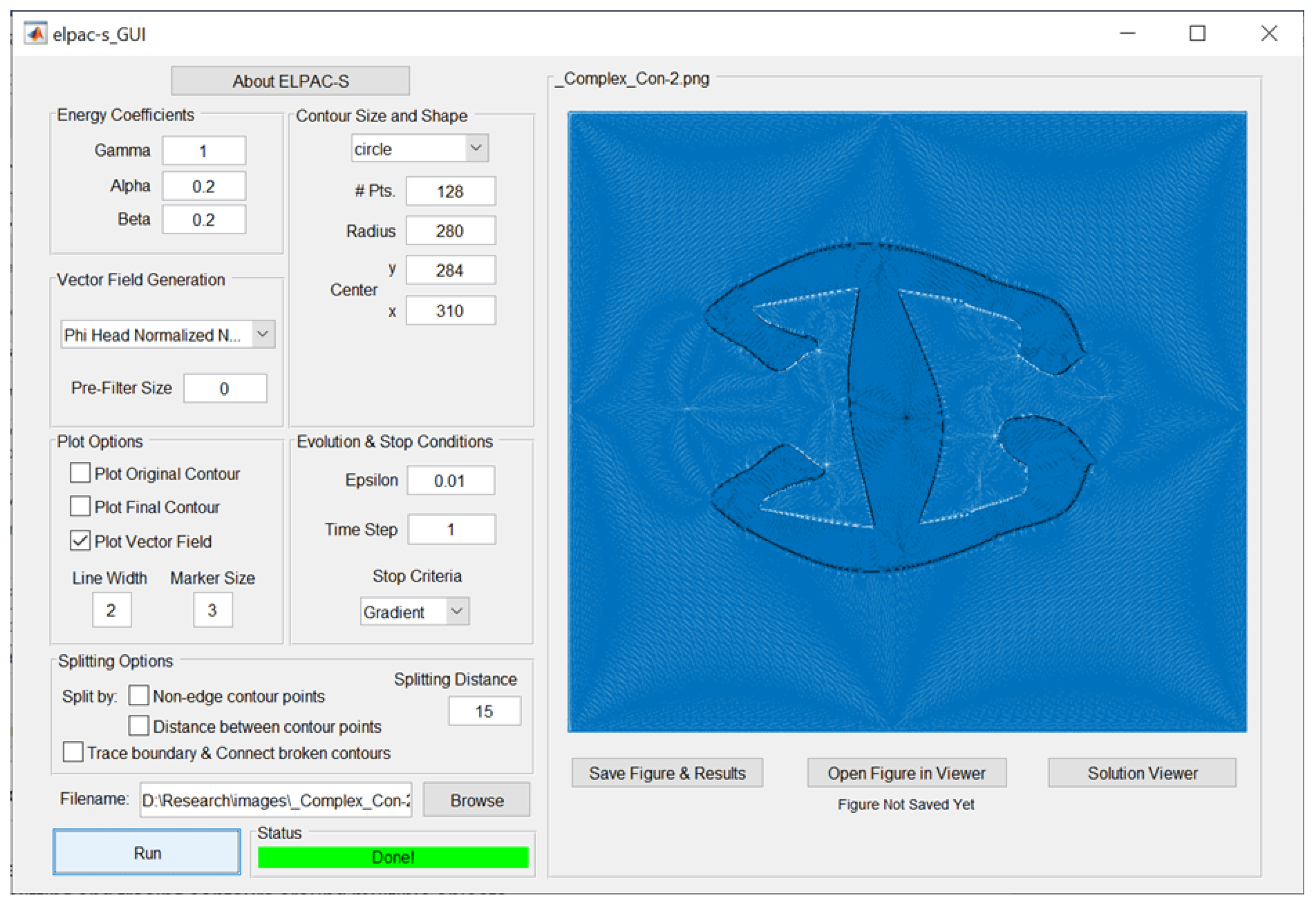
3.3. Software
- Segmenting via an evolving contour directed by the VF . To guide the active contour, with parameters customizable under “Contour Size and Shape”, a VF should be selected from the drop-down menu under “Vector Field Generation”. The recommended choice is “Nabla u Hat”.
- Splitting and tracing contours around multiple objects for full image segmentation. Such options are available under “Splitting Options”.
- Selecting any of the VFs from the “Vector Field Generation” drop-down menu. The six VFs described in Section 2 are at the top of the list. The first three of them have real-shaped SPs [1], while the next three have real- and complex-shaped SPs [3]. The selected VF will be embedded into the image file chosen using the Browse option.
4. Conclusions
- We defined the image regions where the different kinds of SPs will appear, as shown in Table 1.
- We determined the mappings between the SPs of the new VF and the SPs of the VF , formulated in [2, 3], as shown in Figure 8, if the two VFs are separately embedded into the same image.
- We defined a new type of image and image database, named “imprint of an image and imprint of an image database in a VF”.
Author Contributions
Funding
Data Availability Statement
Acknowledgments
Conflicts of Interest
Abbreviations
| ML | machine learning |
| VF | vector field |
| GVF | gradient vector field |
| SP | singular points |
| CP | critical points |
| NN | neural network |
| SRWC | sparse representation wavelet classification |
| SRCQW | sparse representation classification quaternion wavelets |
| CNN | convolutional NN |
| SL | skin lesion |
References
- Sirakov, N.M.; Bowden, A.; Chen, M.; Ngo, L.H.; Luong, M. Embedding vector field into image features to enhance classification. J. Comput. Appl. Math. 2024, 441, 115685. [Google Scholar] [CrossRef]
- Igbasanmi, O.; Sirakov, N.M.; Bowden, A. CNN for Efficient Objects Classification with Embedded Vector Fields. In Computing, Internet of Things and Data Analytics; García Márquez, F.P., Jamil, A., Ramirez, I.S., Eken, S., Hameed, A.A., Eds.; ICCIDA 2023, Studies in Computational Intelligence; Springer: Cham, Switzerland, 2024; Volume 1145, pp. 297–309. [Google Scholar] [CrossRef]
- Igbasanmy, O.D.; Sirakov, N.M. On the Usefulness of the Vector Field Singular Points Shapes for Classification. Int. J. Appl. Comput. Math. 2024, 10, 52. [Google Scholar] [CrossRef]
- Tari, S.; Genctav, M. From a non-local Ambrosio-Tortorelli phase field to a randomized part hierarchy tree. J. Math. Imaging Vis. 2014, 49, 69–86. [Google Scholar] [CrossRef]
- Li, B.; Acton, S. Automatic active model initialization via Poisson inverse gradient. IEEE Trans. Image Process. 2008, 17, 1406–1420. [Google Scholar] [PubMed]
- Ma, J.; Ma, Y.; Zhao, J.; Tian, J. Image Feature Matching via Progressive Vector Field Consensus. IEEE Signal Process. Lett. 2015, 22, 767–771. [Google Scholar] [CrossRef]
- Legaz-Aparicio, A.G.; Verdu-Monedero, R.; Angulo, J. Adaptive morphological filters based on a multiple orientation vector field dependent on image local features. J. Comput. Appl. Math. 2018, 330, 965–981. [Google Scholar] [CrossRef]
- Chen, M.; Sirakov, N.M. Poisson Equation Solution and its Gradient Vector Field to Geometric Features Detection. In Lecture Notes in Computer Science 11324; Fagan, D., Martín-Vide, C., O’Neill, M., Vega-Rodríguez, M.A., Eds.; Springer Nature: Dublin, Irland, 2018; pp. 36–48. [Google Scholar]
- Codella, N.; Rotemberg, V.; Tschandl, P.; Celebi, M.E.; Dusza, S.; Gutman, D.; Helba, B.; Kalloo, A.; Liopyris, K.; Marchetti, M.; et al. Skin Lesion Analysis Toward Melanoma Detection 2018: A Challenge Hosted by the International Skin Imaging Collaboration (ISIC). arXiv 2018, arXiv:1902.03368. [Google Scholar] [CrossRef]
- International Skin Imaging Collaboration. SIIM-ISIC 2020 Challenge Dataset. Internat. Skin Imaging Collaboration. Available online: https://challenge2020.isic-archive.com/ (accessed on 15 May 2023).
- Nene, S.A.; Nayar, S.K.; Murase, H. Columbia Object Image Library (COIL-100); Technical Report; CUCS-006-96. 1996. Available online: http://www1.cs.columbia.edu/CAVE/research/softlib/coil-100.html (accessed on 6 July 2024).
- Georghiades, A.S.; Belhumeur, P.N.; DJKriegman, P.N. From few to many: Illumination cone models for face recognition under variable lighting and pose. IEEE Trans. PAMI 2001, 23, 643–660. [Google Scholar] [CrossRef]
- Digits-MNIST Image Database. Available online: http://yann.lecun.com/exdb/mnist/ (accessed on 3 July 2024).
- Bowden, A.; Sirakov, M.N. Active Contour Directed by the Poisson Gradient Vector Field and Edge Tracking. J. Math. Imaging Vis. 2021, 63, 665–680. Available online: https://rdcu.be/cflaI (accessed on 6 July 2024). [CrossRef]
- Shorten, C.; Khoshgoftaar, T.M. A survey on Image Data Augmentation for Deep Learning. J. Big Data 2019, 6, 60. [Google Scholar] [CrossRef]
- Zhong, Z.; Zheng, L.; Kang, G.; Li, S.; Yang, Y. Random erasing data augmentation. In Proceedings of the AAAI Conference on Artificial Intelligence (AAAI), New York, NY, USA, 7–12 February 2020. [Google Scholar]
- Leevy, J.; Khoshgoftaar, T.; Bauder, R.A.; Seliya, N. A survey on addressing high-class imbalance in big data. J. Big Data 2018, 5, 1–30. [Google Scholar] [CrossRef]
- Wei, L.; Eraldo, R. Detecting Singular Patterns in 2-D Vector Fields Using Weighted Laurent Polynomial. Pattern Recognit. 2012, 45, 3912–3925. [Google Scholar]
- Zhang, E.; Mischaikow, K.; Turk, G. Vector field design on surfaces. ACM Trans. Graph. 2006, 25, 1294–1326. [Google Scholar]
- Sosinsky, A. Vector Fields on the Plane. 2015. Available online: http://ium.mccme.ru/postscript/s16/topology1-Lec7.pdf (accessed on 6 July 2024).
- Argenziano, G.; Soyer, H.; De Giorgi, V. Dermoscopy: A Tutorial; New Media, Edra Medical Pub.: Milan, Italy, 2000. [Google Scholar]
- Siddiqi, K.; Bouix, S.; Tannenbaum, S.W. Hamilton–Jacobi skeletons. Int. J. Comput. Vis. 2002, 48, 215–231. [Google Scholar] [CrossRef]
- Bina, T.; Yib, L. CNN-based flow field feature visualization method. Int. J. Perform. Eng. 2018, 14, 434–444. [Google Scholar] [CrossRef]


| VF | SP/Location | SP/Location | SP/Location |
|---|---|---|---|
| saddle/core | sinking/concavity corners | ||
| saddle/core, branches, concavities | sink/convex vertices, edges | spring/core | |
| saddle/core, branches, concavities | sink/core | spring/edges, convex vertices | |
| saddle/core | sink/core | spring/core; | |
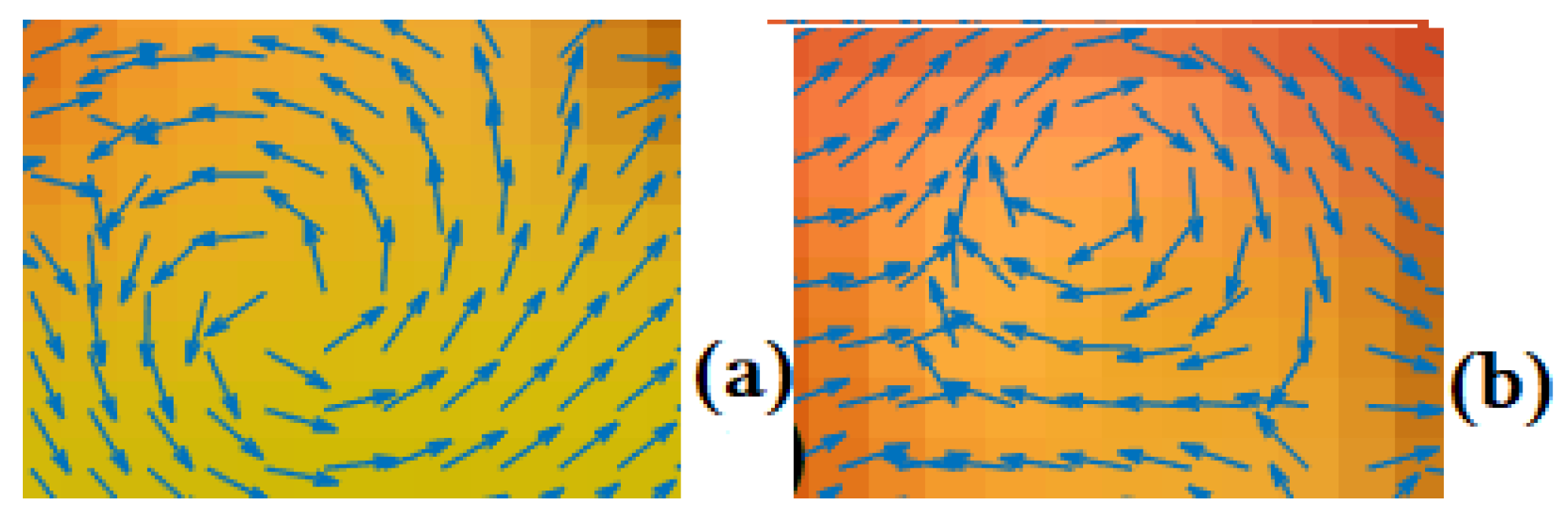
| spiral (in and out)/core | orbits/homogeneous regions | ||
| , | saddle/core, convex vertices | sink/core, edges, branches | spring/core, edges, branches |
| , | spiral (in and out)/core, concavities, branches | orbits/homogeneous regions |
Disclaimer/Publisher’s Note: The statements, opinions and data contained in all publications are solely those of the individual author(s) and contributor(s) and not of MDPI and/or the editor(s). MDPI and/or the editor(s) disclaim responsibility for any injury to people or property resulting from any ideas, methods, instructions or products referred to in the content. |
© 2024 by the authors. Licensee MDPI, Basel, Switzerland. This article is an open access article distributed under the terms and conditions of the Creative Commons Attribution (CC BY) license (https://creativecommons.org/licenses/by/4.0/).
Share and Cite
Sirakov, N.M.; Bowden, A. Image Databases with Features Augmented with Singular-Point Shapes to Enhance Machine Learning. Electronics 2024, 13, 3150. https://doi.org/10.3390/electronics13163150
Sirakov NM, Bowden A. Image Databases with Features Augmented with Singular-Point Shapes to Enhance Machine Learning. Electronics. 2024; 13(16):3150. https://doi.org/10.3390/electronics13163150
Chicago/Turabian StyleSirakov, Nikolay Metodiev, and Adam Bowden. 2024. "Image Databases with Features Augmented with Singular-Point Shapes to Enhance Machine Learning" Electronics 13, no. 16: 3150. https://doi.org/10.3390/electronics13163150