A Fault Diagnosis Method for Electric Check Valve Based on ResNet-ELM with Adaptive Focal Loss

Abstract

Under the trend of carbon neutrality, the adoption of electric mineral transportation equipment is steadily increasing. Accurate monitoring of the operational status of electric check valves in diaphragm pumps is crucial for ensuring transportation safety. However, accurately identifying the operational characteristics of electric check valves under complex excitation and noisy environments remains challenging. This paper proposes a monitoring method for the status of electric check valves based on the integration of Adaptive Focal Loss (AFL) with residual networks and Extreme Learning Machines (AFL-ResNet-ELMs). Firstly, to address the issue of unclear feature representation in one-dimensional vibration signals, grayscale operations are employed to transform the one-dimensional data into grayscale images with more distinct features. Residual networks are then utilized to extract the state features of the check valve, with Extreme Learning Machines serving as the feature classifier. Secondly, to overcome the issue of imbalanced industrial data distribution, a new Adaptive Focal Loss function is designed. This function focuses the training process on difficult-to-classify data samples, balancing the recognition difficulty across different samples. Finally, experimental studies are conducted using industrially measured vibration data of the electric check valve. The results indicate that the proposed method achieves an average accuracy of 99.60% in identifying four health states of the check valve. This method provides a novel approach for the safety monitoring of slurry pipeline transportation processes.

1. Introduction

1.1. Background

With the transformation of industrial automation, slurry pipeline transportation has emerged as a novel method for ore transportation. The diaphragm pump, as its core power unit, efficiently manages slurry transportation under conditions of high pressure, high temperature, and high corrosiveness, offering an effective solution to the challenges of long-distance slurry transportation [1]. Among the components of the diaphragm pump, the check valve, which undergoes the most frequent movement, is characterized by rapid opening and closing, sealing, and high-pressure bearing under the complex excitation of slurry and the diaphragm pump over extended periods. Consequently, check valves are more prone to failure than other parts of the diaphragm pump [2], and such failures can impact other components, leading to a series of production safety and economic issues. In order to reduce the occurrence of slurry transportation system failures, enterprises often adopt the method of regular maintenance (1200 h regular replacement of check valves), but excessive maintenance will cause downtime losses and waste of maintenance resources, and insufficient maintenance may lead to safety accidents, resulting in greater losses. There is also a disadvantage in regular maintenance: some check valves (effective working time of 2000 h to 3000 h) can still operate safely for a long time after reaching the preset operating time, and some check valves fail before reaching the preset operating time, which easily causes waste of maintenance resources and safety accidents. The fault diagnosis and maintenance of check valves urgently need an accurate and reliable judgment basis, and preventive maintenance can ensure the safety and reliability of diaphragm pump operation, reduce maintenance costs, and improve production efficiency. The operation status monitoring method of diaphragm pump check valve has become an urgent need of metallurgical enterprises. The purpose of the research is to identify the operation status of the check valve to ensure the stable operation of the diaphragm pump, improve production efficiency and reduce maintenance costs, and avoid economic losses and other more serious accidents. Therefore, it is of significant importance to carry out the research on the operation status monitoring of diaphragm pump check valves for the supply of mineral raw materials and even for the metallurgical industry.

1.2. Status of the Research on Fault Diagnosis of Check Valves

Traditionally, fault diagnosis methods have relied on the analysis and processing of measured signals [3], allowing the determination of the location, type, and severity of mechanical faults through theoretical calculations or empirical knowledge comparison [4,5]. Zhou et al. [6] proposed a check valve fault diagnosis method combining complementary ensemble empirical mode decomposition, fundamental scale entropy, and fuzzy c-means clustering. Pan et al. [7] introduced a method based on parameter optimized variational mode decomposition and enhanced multiscale permutation entropy, while Chen et al. [8] developed a method utilizing a mean dispersion negative entropy infograph. In the realm of reciprocating mechanical fault diagnosis, Zhao et al. [9] proposed a composite interpolation envelope local mean decomposition to address the gap fault problem in reciprocating compressors. Xia et al. [10] extracted fault characteristics of the reciprocating pump plunger by analyzing the synchronous power spectrum of the reciprocating pump plunger signal in time, amplitude, and frequency domains, successfully diagnosing the reciprocating pump plunger. However, few signal processing-based fault diagnosis methods possess absolute advantages over others, as these algorithms fundamentally involve mathematical operations [11]. Consequently, the choice of methods largely depends on the performance characteristics of the original signal and the research objectives.

Data-driven fault diagnosis research offers more innovative approaches due to its robust capability to extract historical data features [12,13]. In particular, the ELM network applied in this paper is a single-layer feedforward neural network [14], which has the advantages of fast learning and good generalization performance compared with traditional classification methods, and does not need to repeatedly adjust the hidden layer parameters, and has also been applied by many scholars. Li et al. [15] employed multi-scale permutation entropy to extract time-domain information of check valves and established a working condition recognition model using Extreme Learning Machines (ELMs). Ma et al. [16] proposed a fault diagnosis method for checking valves based on a multi-core cost-sensitive ELM. Xu et al. [17] utilized the principal component autoregressive method to extract fault features and applied neural networks for fault diagnosis of reciprocating pumps. Chen et al. [18] combined cyclic spectral coherence with convolutional neural networks (CNNs) to create a new rolling bearing fault diagnosis scheme, achieving superior classification performance. Bie et al. [19] constructed eigenvectors using singular spectral entropy and applied long short-term memory networks (LSTMs) to extract fault features from reciprocating pump vibration signals. Wei et al. [20] combined LSTMs with a one-dimensional convolutional neural network to diagnose high-speed axial piston pumps. Chen et al. [21] used deep neural networks for fault identification of rolling bearings under strong interference, attaining high recognition accuracy. Li et al. [22] proposed a method for diagnosing the liquid end of a drilling pump based on an extended AlexNet model. Janssen et al. [23], from Ghent University, developed a condition monitoring feature learning model using convolutional neural networks, demonstrating 93.61% accuracy in diagnosing various bearing faults. These studies indicate that data-driven fault diagnosis methods excel in uncovering hidden data correlations, reducing manual labeling, and enhancing signal feature extraction and pattern recognition [24,25].

A common issue in fault diagnosis research is the imbalance in data distribution, where mechanical equipment typically operates in a normal state, resulting in abundant healthy state data but scarce fault state data [26,27]. This imbalance causes convolutional networks to favor normal conditions [28], leading to inadequate understanding of the characteristics of the abnormal state of the check valve, potentially resulting in misclassification, missed maintenance opportunities, and significant economic losses. To address data imbalance, techniques such as the Minority Sample Oversampling Synthesis Technique (SMOTE) [29] balance datasets by generating virtual samples for minority classes, while cost–loss algorithms [30,31] such as weighted cross-entropy (CE) and focal loss (FL) adjust weights to balance the impact of different categories on losses [32,33]. However, methods such as SMOTE may produce erroneous samples under varying spatial and operational conditions [34]. However, FL was originally proposed to be used for dense object detection tasks; for example, in object detection, there may be 1000 classes of objects to be detected, but the object one wants to identify is only one of them, so it is actually a classification problem with a very uneven sample [35]. To put it simply, it solves the problem of extreme imbalance in the number of samples, and the advantage is that, on the basis of not generating samples, it is integrated into the network layer to solve the problem of sample imbalance, directly paying more attention to the samples that are difficult to classify, and at the same time reducing the impact on the easy-to-classify samples, so as to improve the performance of the model on the category imbalance data [36].

According to different survey results, data-driven fault diagnosis research is one of the popular research directions in this field [37,38]. Convolutional neural networks have become the first choice for many fault diagnosis research methods due to their excellent data and information mining capabilities [39]. Because traditional convolutional neural networks are prone to the problems of Vanishing Gradient and Exploding Gradient when the number of network layers continues to deepen, it is difficult to train. Compared with traditional neural networks, the main difference between ResNet and ResNet is the introduction of Skip Connection and the use of residual learning. This structure improves the network’s optimization performance and allows for deeper levels, which greatly improves the training efficiency and generalization ability of the network.

To mitigate the risks posed by check valve failure to the entire slurry transportation system, this paper proposes a check valve condition monitoring method that combines residual networks with ELM. The residual network extracts data features, and the ELM serves as the classifier to enhance the generalization and training speed of the algorithm. Additionally, to address the imbalance in data collected from different operating states of check valves, the Adaptive Focal Loss (AFL) is designed to apply adaptive difference weighting to check valve operation states. This approach reduces dependency on the loss function, mitigates the impact of data imbalance, and improves the monitoring accuracy of the proposed model. Furthermore, this method ensures high recognition accuracy for both the health criticality and fault states of the check valve, a core focus of this paper.

1.3. Contributions and Structure

This paper makes significant contributions in the following areas:

(a)

Addressing the health monitoring requirements of check valves, we propose a check valve condition monitoring model that combines residual networks and ELMs. This model extracts features using the residual network and employs ELMs for feature identification, achieving high-precision monitoring of the operational status of check valves.

(b)

To tackle the issue of extreme imbalance in the check valve dataset, we introduce the Adaptive Weighted FL. This method improves the accuracy of identifying check valve faults or other abnormal states, mitigates the impact of data imbalance, and ensures the core objectives of this study.

The rest of this article is organized as follows: Section 2 introduces some fundamental theoretical backgrounds and presents the design method for AFL and the ResNet-ELM condition monitoring model. Section 3 details the experimental background and setup. In Section 4, the effectiveness of the proposed method is verified and analyzed. Finally, Section 5 summarizes the article. The research path of this study is illustrated in Figure 1.

2. Methods

The method proposed in this paper involves ResNet, ELM, and FL. Therefore, a brief introduction to these concepts is provided before presenting the fault diagnosis framework, followed by a detailed discussion of the proposed methods.

2.1. Proposed of the ResNet and ELM Model

2.1.1. Proposed of the ResNet

CNNs are a fundamental component of residual networks (ResNet) [40,41]. CNNs typically consist of convolutional layers, pooling layers, and fully connected layers. Convolutional layers, which are crucial modules of CNNs, usually comprise a set of convolutional kernels (or filters) and corresponding biases. Each channel’s convolution kernel generates a nonlinear feature map by applying a convolution operation, followed by a nonlinear activation function. The mathematical formula for convolutional layer operations is expressed as follows [42]:

$$Z_j^l=\mathrm{\delta }\left(\sum _i{x}_i^{l-1}\ast {\omega }_{ij}^{l-1}+b_j^l\right)$$

(1)

where ∗ is convolution operations; $x_i^{l-1}\left(l-1\right)\mathrm{t}\mathrm{h}$ is the feature mapping of the $i$th channel in the $\left(l-1\right)\mathrm{t}\mathrm{h}$ layer; ${\omega }_{ij}^{l-1}$ and $b_j^l$ are the convolution kernels and biases corresponding to the $j$th channel, respectively. $Z_j^l$ is represented as a feature map of the $j$th channel of the $l$th layer; $\mathrm{\delta }$ represents a nonlinear activation function, and the commonly used activation function is the (Rectified Linear Unit) ReLU function used in this article.

The pooling layer’s function is to reduce the input dimension and the number of parameters, which helps decrease computation and improve network generalization. Its mathematical formula is the following:

$$Z_j^l=\mathrm{d}\mathrm{o}\mathrm{w}\mathrm{n}\left(x_j^{l-1}\right)$$

(2)

where $\mathrm{d}\mathrm{o}\mathrm{w}\mathrm{n}\left(·\right)$ represents a pooling function or a dimensionality reduction sampling method. Regularization operations are often employed in convolutional networks [43] to enhance network performance. The batch normalization layer standardizes the input maps in batches, and its mathematical calculation formula is the following:

$$\widehat{x}=\mathrm{B}\mathrm{N}\left(x\right)={\displaystyle \frac{x-mean\left(x\right)}{\sqrt{Var\left(x\right)-eps}}}\times \mathrm{\upsilon }+\rho$$

(3)

where $\widehat{x}$ is the normalized output of the matrix; eps is the stability factor, which is a decimal close to zero, and the default is 10⁻⁵; $\mathrm{\upsilon }$ and $\rho$ are the backpropagation adjustment coefficients, which are used to optimize the network model in order to make full use of the feature extraction ability of convolutional neural network and overcome the network degradation problem caused by the deepening of network layers.

Figure 2 illustrates a basic residual block structure of ResNet [44]. In this study, the residual network is used as the primary model framework for feature extraction. A basic residual block, as shown in Figure 2 [45], comprises two “Conv-BN-ReLU” structures connected in series and then connected in parallel, with a shortcut connection to form a basic residual module.

2.1.2. Brief Introduction of ELM

The ELM operates as a classifier with hidden weights that are randomly generated and remain fixed during training, eliminating the need for further adjustment. The ELM optimization is achieved by minimizing the norm of training errors and output weights, as shown in Equation (4), demonstrating a robust generalization performance for hidden data information, according to Bartlett [46]. In the process of model training, the training error is used as the judgment criterion, and the training error usually decreases with the increase in the number of hidden nodes. This is because more hidden nodes provide a larger model capacity and are able to better fit the training data.

$$\min ({\displaystyle \frac{1}{2}}{\parallel \beta \parallel }^2+{\displaystyle \frac{C}{2}}{\parallel T-H\beta \parallel }^2)$$

(4)

where the first term is the norm of the weight, and the second term is the training error. C is the penalty coefficient that controls the two trade-offs. $T=\left[t_1,t_2,\cdots ,t_m\right]$ is the target matrix of the training samples used, and $\beta$ is the output weight matrix connecting the nodes of the output layer and the nodes of the hidden layer.

For an input $x=\left[x_1,x_2,x_3,···,x_m\right]$, and the ELM’s hidden layer contains L hidden nodes, then the hidden layer input corresponding to the ELM’s nonlinear feature map is $x=\left[h\left(x_1\right),h\left(x_2\right),h\left(x_3\right),···,h\left(x_L\right)\right]$. If the number of hidden nodes is too small, the model may not be able to capture the complexity of the data, and the training accuracy of the ELM may be low, resulting in underfitting. If the number of hidden nodes is too large, the training accuracy of the ELM may reach a very high level, but this does not necessarily mean that the generalization performance will improve, which may lead to overfitting. Therefore, the ELM can fit the training data well only when the number of hidden nodes is reasonable during the training process.

Thus, the mathematical formula for the ELM output mapping is the following:

$$Z_i=\sum _{i=1}^L{\beta }_i·h\left(x_i\right)=h\left(x_j\right)·\beta j=\mathrm{1,2},\cdots ,m$$

(5)

where $\beta =\left[{\beta }_1,{\beta }_2,\cdots ,{\beta }_L\right]$; $Z_i$ is the output of the ELM. The ELM structure is shown in Figure 3.

Since the weights and biases of the ELM are randomly generated, the output of the hidden layer node is the following:

$$H=\left[\begin{array}{c}h\left(x_1\right)\\ ⋮\\ h\left(x_m\right)\end{array}\right]=\left[\begin{array}{ccc}{h}_1\left({\omega }_1^T{x}_1+b_1\right),& \cdots & ,h_L\left({\omega }_L^T{x}_1+b_L\right)\\ ⋮& ⋮& ⋮\\ h_1\left({\omega }_1^T{x}_m+b_1\right),& \cdots & h_L\left({\omega }_L^T{x}_m+b_L\right)\end{array}\right]$$

(6)

According to the optimization function shown in Equation (4), the output weight matrix $\beta$ is solved by minimizing the approximation error of the output weight matrix and the training samples.

Firstly, if the number of training samples $m$ is greater than the number of hidden nodes L, i.e., the number of rows of the hidden output matrix $H$ is greater than the number of columns, Huang [47] provides a least-squares solution of the minimum norm of the $\beta$, ${\beta }^{\ast }=H^{+}T$, where $H^{+}$ is the Moore–Penrose generalized inverse of the matrix H. By setting the gradient of the Lagrangian equation to zero, we get the following:

$${\beta }^{\ast }-C{H}^T\left(T-H{\beta }^{\ast }\right)=0$$

(7)

Then, $\beta$ can be expressed as follows:

$${\beta }^{\ast }=H^{+}T={\left(H^{T}H+{\displaystyle \frac{L}{C}}\right)}^{-1}{H}^{T}T$$

(8)

where $T$ is the identity matrix of the L dimension. Since $H$ is the full rank of the column, then $H^{T}H$ is an invertible matrix, and it can be seen that when the gradient of the optimization function is zero, the training error of the ELM reaches the minimum. As a result, the ELM is astringent.

Secondly, if the number of training data $m$ is less than the number of hidden nodes L, the orthogonal projection method of SVD decomposition can be used to calculate the Moore–Penrose generalized inverse of the matrix $H$, when $H{H}^T$ is not singular, $H^{+}=H^T{\left(H^{T}H\right)}^{-1}$, and $\beta$ can be expressed as follows:

$${\beta }^{\ast }=H^{+}T=H^T{\left(H^{T}H+{\displaystyle \frac{L}{C}}\right)}^{-1}T$$

(9)

where ${\beta }^{\ast }$ is the only solution of the optimization function, so the ELM not only achieves the smallest training error but also obtains the smallest weight norm. Under these conditions, the ELM also converges. The output value of the input test sample is calculated as follows:

$$Z=h\left(x\right){\beta }^{\ast }=\left\{\begin{array}{c}h\left(x\right)·\left({\left(H^{T}H+{\displaystyle \frac{L}{C}}\right)}^{-1}{H}^{T}T\right) if m\ge L\\ h\left(x\right)·{(H^T\left(H^{T}H+{\displaystyle \frac{L}{C}}\right)}^{-1}T) if m<L\end{array}\right.$$

(10)

2.1.3. The Development of ResNet-ELM Model

The basic model framework employed in this paper is the 18-layer structure of ResNet, which primarily consists of an input layer, batch normalization, activation functions, residual modules, pooling layers, fully connected layers, a softmax layer, and an output layer [48,49]. The residual module comprises several basic residual blocks, as illustrated in Figure 4. To enhance the model’s feature classification capability, the softmax layer in ResNet has been replaced with the ELM. This substitution improves generalization performance due to the ELM’s optimization method of minimizing the output weight matrix and training error.

The network model in this study is described as using a residual network for feature extraction and an ELM for feature classification, forming the ResNet-ELM framework. The proposed model, ResNet-ELM, is depicted in Figure 5. In the input layer, the grayscale image transformed from the vibration signal is used as the input [50] because the transformed grayscale image is more easily learned by the two-dimensional convolutional network compared to the original one-dimensional vibration signal. After the grayscale image is processed by the residual network, the high-dimensional features are input into the ELM for check valve state recognition, resulting in the status monitoring outcomes of the check valve.

As can be seen from the above model structure diagram, ResNet-18 uses multiple residual blocks, each containing multiple convolutional layers (usually 3 × 3 convolutional kernels), which gradually extract the high-level features of the image through the layer-by-layer processing of the feature map. Convolutional layers have local receptive fields that capture local patterns and features in the image. In ResNet, the residual connection allows the network to maintain the flow of the gradient as the depth increases, avoiding the problem of vanishing gradients, thus improving the training stability of the model. And each residual block helps the network learn features better by adding shortcut connections. Since the residual block allows for the direct skipping of one or more layers, this structure can reduce information loss and make the model more robust for feature learning. When interpreting the model, the contribution of the residual blocks to the feature extraction can be analyzed to understand the impact of each residual block on the final feature. At the same time, as a classifier with good generalization ability, the learning process of the ELM includes randomly initializing the weights of the hidden layer, and then training the model by minimizing the output weight matrix and training error. Because the training process of the ELM is simple, and the mathematical principle is clear, its weight calculation process can help understand the classification decision of the model, and the output weight matrix of the ELM is directly related to the feature vector, so the classification results of the model can be solved by analyzing these weight matrices.

Therefore, in the ResNet-ELM framework, the high-dimensional features extracted by ResNet are first imported into the ELM for classification, and by analyzing the relationship between these features and the output weights of the ELM, it can be understood that the model classifies according to the features of different dimensions of the image, thereby increasing the interpretability of the type.

2.2. Improved ResNet-ELM with AFL

2.2.1. Brief Introduction of FL

FL is employed to address the issue of data imbalance between positive and negative samples in object detection [51]. This loss function mitigates the influence of negative samples during model training, making it an effective method for handling imbalanced data. Due to the large number of negative samples, their training loss often dominates the total loss, making the classification of negative samples easier, while the model struggles to accurately identify positive samples. In such cases, the model’s optimization direction does not align with actual needs [52,53]. The FL function is based on the CE loss function and adjusts the model to focus more on difficult-to-classify samples by reducing the weight of correctly classified samples. To introduce FL, we start with the binary classification CE loss [33]:

$$C{E}_2(p,y)=\left\{\begin{array}{c}-\log (p)\hspace{0.17em}if y=1\\ -\log (1-p)\hspace{0.17em}otherwise\end{array}\right.$$

(11)

where p is the probability that the predicted sample is true; $y$ is the tag value. To change the binary CE function to a multi-categorical CE function, first rewrite p to $p_t$, as shown in the following equation:

$$p_t=\left\{\begin{array}{c}p\hspace{0.17em}if y=1\\ 1-p\hspace{0.17em}otherwise\end{array}\right.$$

(12)

If $p_t$ represents the probability that the predicted sample is a true classification, the multi-classification CE function is rewritten from Equation (11) as follows:

$$CE(p,y)=CE(p_t)=-\log (p_t)$$

(13)

A common way to solve the imbalance of data classes is to introduce a weight factor in the loss function for different classes $\alpha =[{\alpha }_1,{\alpha }_2,\dots ,{\alpha }_n]$. By assigning the proportion of positive and negative samples to the total training loss by the weight factor, the contribution of the positive samples in the training loss is increased, the proportion of negative samples in the training loss is reduced, and the weighted CE loss is described as follows:

$$CE(p_t)=-\alpha \log (p_t)$$

(14)

While the weighted CE can control the weights of positive and negative samples, it does not differentiate between difficult and easily classified samples. Therefore, to address this, the FL function introduces a modulation factor that reduces the contribution of high-confidence samples in the loss function and increases the proportion of low-confidence samples, thereby focusing on difficult samples. The CE function with an added modulation factor is expressed as follows:

$$FL(p_t)=-{(1-p_t)}^{\gamma }\log (p_t)$$

(15)

where $\gamma$ is expressed as the focus parameter, $\gamma$ ≥ 0 and $(1-p_t)$ is expressed as a modulation factor. In order to consider the “easy to distinguish” and “positive and negative samples” problems together, we propose an improved approach. To sum up, the final expression for FL is as follows:

$$FL(p_t)=-{\alpha }_t{(1-p_t)}^{\gamma }\log (p_t)$$

(16)

The experimental results have shown that when $\gamma$ = 2, FL has a good performance, and it is worth discussing the reasonable design of the α value to adapt to the contribution of positive and negative samples in the total loss.

2.2.2. AFL for Data Class Imbalance

Although the basic FL function can differentiate the importance of various samples, it struggles to handle the imbalance in sample size across categories. Therefore, this section proposes an AFL method to address sample imbalance based on cost loss.

Firstly, rebalancing the sample loss contribution rate of positive and negative samples during feedback learning helps mitigate the influence of data volume proportion on the model. To set the weight factor ${\alpha }_t$ reasonably, an effective weighting factor calculation method is essential. This paper proposes a weighting method that focuses on the ratio of different types of data. The mathematical formula for this method is expressed as follows:

$${\alpha }_t={\alpha }_0\times {\left(\sqrt{{\displaystyle \frac{{\lambda }_{max}}{{\lambda }_t}}}\right)}^{\phi }$$

(17)

where $\phi$ is the weighted factor modulation factor, and the value of $\phi$ is often designed as 1. ${\alpha }_0$ is the initial weight, the design value of the class with the largest amount of data is 0.5, and ${\lambda }_t$ is the proportion of class t in the overall data. In this method, adding a square root to the method of data volume ratio can avoid over-expanding the sample loss proportion of part of the data volume, but reduce the overall test sample accuracy. At the same time, the square root is very sensitive to the size of a set of data errors, so the square root can effectively reflect the accuracy of the measurement, so that the weight factor of the design has better adaptability.

Secondly, if the proportion of negative samples is extremely exaggerated, the reasonable setting of the weight factor ${\alpha }_t$ can solve a part of the problem, but due to the “accumulation” of negative sample loss, it will still account for a large part of the sample loss, since negative and easy samples highly overlap in data classification. The core content of the FL function for difficult and easy sample processing is the $\gamma$ of focal length parameters. The value of $\gamma$ has a great impact on the training of different samples. When $\gamma$ = 0, the FL function is the CE function. With the training and learning process of the model, the boundary between the difficult and easy samples of the model will change, so the value of the reasonable adjustment of the focal length parameter $\gamma$ changes with the model training process, which can make it more consistent with the model training process. Therefore, the dynamic focal length parameter ${\gamma }_{lr}^{\ast }$ is proposed to replace the invariant focal length parameter $\gamma$ in FL and, combined with the setting method of the weight factor ${\alpha }_t$, the AFL function as shown in Equation (20) is finally proposed.

$${\gamma }_{lr}^{\ast }={\gamma }_0\times \sqrt{{\displaystyle \frac{lr}{{lr}_0}}}$$

(18)

$$lr={lr}_0\times {dr}^{{\displaystyle \frac{gs}{ds}}}$$

(19)

$$AFL\left(p_t\right)={-\alpha }_t{\left(1-p_t\right)}^{{\gamma }_{lr}^{\ast }}log\left(p_t\right)$$

(20)

where ${\gamma }_0$ is the initial value of the $\mathsf{\gamma }$, according to the experiment in this paper, ${\gamma }_0$ = 2, ${lr}_0$ is the initial learning rate of model training, ${lr}_0=0.01$, and $lr$ is the attenuation learning rate generated with the model training iteration. $dr$ is the attenuation coefficient of the learning rate, $0<dr<1$, and $ds$ is the decay rate. $gs$ indicates the number of iterations required for a model to complete a full dataset training. With the decay in $lr$, the ${\gamma }_{lr}^{\ast }$ will decay accordingly, ensuring that the loss of the model in the later stage of training does not become too small, thereby preventing a significant weakening of the learning ability of the model. The AFL function is not only reasonably designed in terms of the weight factors of positive and negative samples; its parameter, ${\gamma }_{lr}^{\ast },$ is related to the learning rate, which can maintain better learning ability in the later learning, so it has better generalization.

2.2.3. Improved ResNet-ELM Model

In the context of this study, the collected data contain a substantial number of samples representing normal health statuses, whereas samples indicative of check valve failures or critical faults are markedly scarce. This imbalance creates a significant practical challenge, as traditional neural network models are prone to overfitting on the abundant samples from the majority class. Consequently, features of the minority class may be underrepresented, leading to reduced performance in detecting rare anomalies.

Addressing this issue, the focus of this paper is on precise monitoring of check valve failures and other anomalies. Traditional neural network models fail to adequately meet these needs due to their inability to effectively handle class imbalance. To overcome this limitation, an improved model, denoted as the AFL-ResNet-ELM, is proposed. This model utilizes the ResNet-ELM for feature extraction and classification, and incorporates AFL to address the imbalance in sample difficulty. The AFL-ResNet-ELM model adaptively adjusts the focus on challenging versus easily classified samples and modifies the contribution rate of data samples during feedback learning to enhance the generalization capability of the neural network. Let the training set be set to ${\left\{x^q,y^q\right\}}_{q=1}^Q$, where $x^q$ represents the sample of the training set $q\mathrm{th}$ and $y^q\in \left\{\mathrm{1,2},...,C\right\}$ represents the target category of mechanical health. From Equation (20), the loss of the training sample can be calculated as follows:

$$l_{AFL}=-{\displaystyle \frac{1}{Q}}{\displaystyle \sum _{q=1}^Q{\displaystyle \sum _{c=1}^C{\alpha }_{c}1\left\{y^{(q)}=c\right\}}}{(1-p_c)}^{{\gamma }_{lr}^{*}}\log (p_c)$$

(21)

where $1\left\{·\right\}$ represents the pointer function; if the condition is true, it returns 1; otherwise, it returns 0. Further, $l_{AFL}$ is a partial derivative of the parameter $p$:

$$L_{pd}={\displaystyle \frac{\partial l_{AFL}}{\partial p_c}}=-{\displaystyle \frac{1}{Q}}{\displaystyle \sum _{q=1}^Q{\alpha }_{c}1\left\{y^{(q)}=c\right\}}(-{\gamma }_{lr}^{*}{(1-p_c)}^{{\gamma }_{lr}^{*}-1}\log (p_c)+{(1-p_c)}^{{\gamma }_{lr}^{*}}{\displaystyle \frac{1}{p_c}})$$

(22)

Since the $p_c$ correctly identifies the proportion of category output in the total output of the model, the change law of $L_{pd}$ reflects the change of learning gradient in model feedback learning to a certain extent. Among them, ${\alpha }_c$ can enhance or weaken the gradient proportion of a certain type of data in feedback learning; ${\gamma }_{lr}^{\ast }$ makes the model pay more attention to difficult samples, due to the iterative learning of the model, the division boundary of the classification changes, and ${\gamma }_{lr}^{\ast }$ decays with the attenuation of the learning rate, which ensures the continuous learning ability of model training, with AFL-ResNet-ELM exhibiting certain advantages in model learning optimization.

2.3. Check Valve Conditions Monitoring Method Based on AFL-ResNet-ELM

It is important to note that prior to training the ELM, the initial network parameters of the ResNet model are generated randomly, which may not effectively capture the features of the input data. Consequently, the ResNet model is pre-trained using the training dataset to ensure that high-dimensional features are adequately extracted. These features are then utilized as inputs for the ELM model once certain conditions are met. In this study, the ELM model is trained after the accuracy of the ResNet model remains unchanged over several consecutive training iterations or reaches the predefined maximum number of training epochs. The proposed condition monitoring scheme for check valves is illustrated in Figure 6, and the specific steps are outlined as follows:

Step 1: data acquisition. The first step involves measuring the vibration signal of the check valve using an accelerometer.

Step 2: data preprocessing. The recorded one-dimensional time series signal is analyzed and classified. It is then transformed into a two-dimensional grayscale image through grayscale image transformation techniques, with the dimensions of the image set to 64 × 64 pixels.

Step 3: model training. The dataset is divided into training and test sets. The ResNet model’s architecture is defined and pre-trained on the training dataset. During this pre-training phase, the AFL function is employed as the optimization criterion to enhance the model’s ability to handle class imbalance and focus on difficult samples.

Step 4: feature extraction and classification. An ELM network model is constructed, and key parameters, such as the number of hidden nodes (L) and the penalty coefficient, (C) are set. The pre-trained ResNet model is used to generate feature maps from the training set data, which are then combined and used as input for the ELM model. The ELM model is trained using these features through the generalized inverse method to perform classification.

Step 5: testing. For evaluation, the test samples are fed into the trained the AFL-ResNet-ELM model to produce the final diagnostic results.

The implementation and optimization of the entire methodology are carried out using Python (version 3.10) and the PyTorch (version 1.10.1) framework. The computational processes are supported by an AMD 5600X (Advanced Micro Devices, Taiwan, China) processor and an NVIDIA GeForce GTX 1060 GPU (NVIDIA Corporation, Santa Clara, California, USA), which help reduce training and optimization times.

3. Experimental Testing

3.1. Data Collection Schemes

This study focuses on the TZPM series three-cylinder crankshaft-driven piston diaphragm pump, which incorporates three sets of inlet and outlet check valves. The whole diaphragm pump system mainly includes diaphragm pumps, check valves and other auxiliary equipment. In order to ensure the normal operation of the diaphragm pump system in use and find the abnormal state of the valve body in time, the vibration sensor is arranged on the housing of the check valve (including two check valves at the entrance and exit, for a total of 6 groups), and the data collection system is used to collect the vibration acceleration time domain signal on the check valve housing to monitor the operation status of the check valve in real time. The specific sensor location and data acquisition scheme are shown in Figure 7. The experiment was carried out under the actual industrial production. The stroke number of the diaphragm pump was 30 times/min~31 times/min, the operating frequency was 0.5–0.517 Hz, the equipment sampling frequency was 2.56 kHZ, and the single sampling time was 3 s.

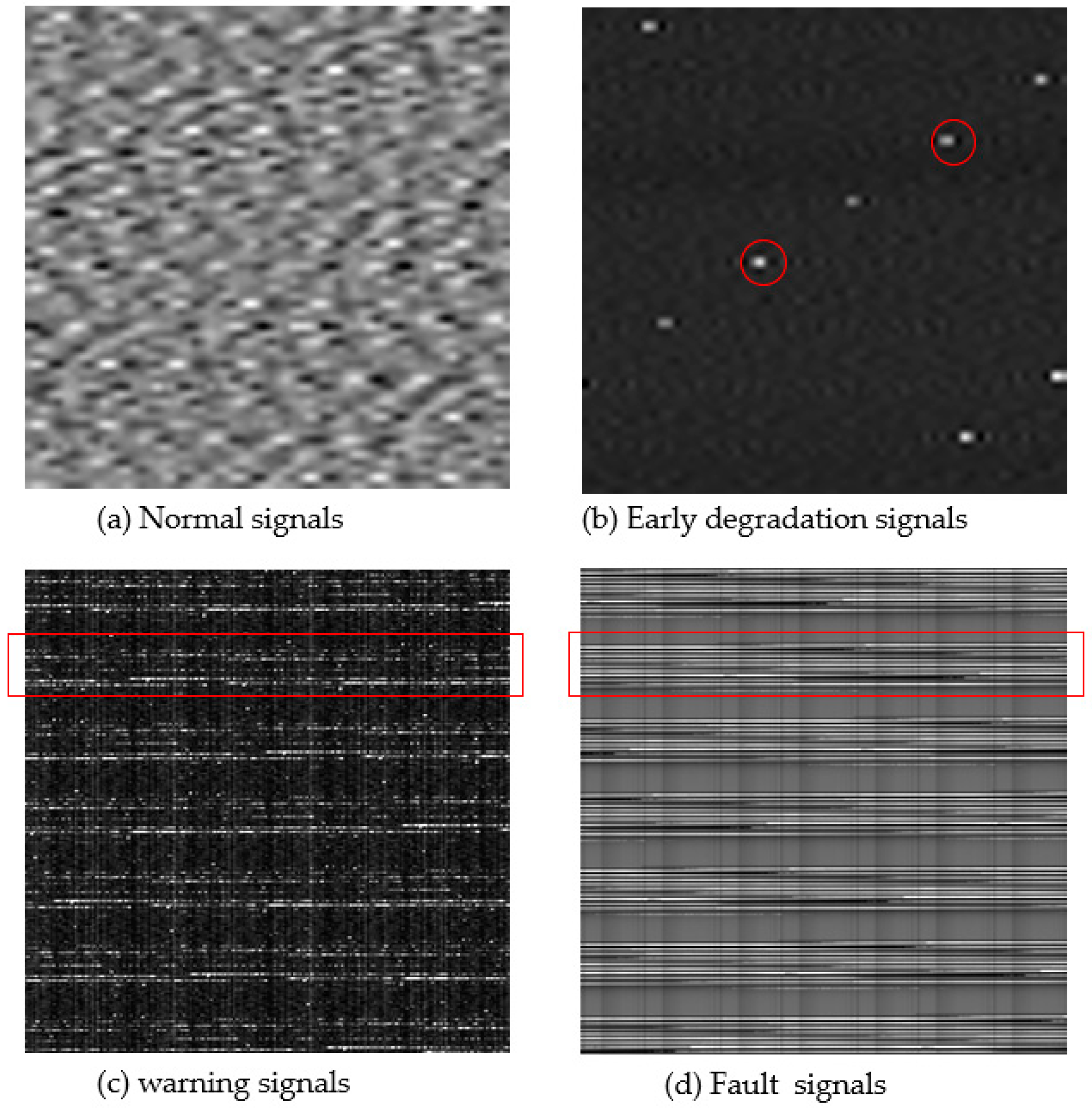
3.2. Vibration Signal Analysis of Check Valves

The failure modes of check valves can be categorized into several conditions based on their underlying causes. These include the following:

(1)

Normal operation: in this state, both the diaphragm pump and the check valve function properly, and the vibration signal from the valve body appears as a periodic random signal.

(2)

Early degradation: while the diaphragm pump continues to operate reliably, the check valve experiences minor wear, resulting in a pulsed vibration signal indicative of the valve’s reciprocating motion.

(3)

Fault warning: This condition is typically characterized by severe scratching on the valve due to the presence of high-hardness particles in the slurry or continuous impact on the valve sealing surface. The vibration signal in this state is often represented by a multi-peak strong pulse signal or a pronounced noise signal.

(4)

Equipment failure: This state indicates significant breakdown or deformation of the valve body at the sealing surface. The corresponding vibration signal is a high-intensity, multi-peak periodic pulse signal.

The operational states of the check valve are illustrated in Figure 8.

3.3. Dataset Analysis

The dataset employed in this study was derived from industrial measurements and encompasses data samples from four distinct check valve operating states. The detailed categories of these states are presented in

Table 1. Percentage of individual health status data.

Label	Normal	Early Degradation	Warning	Fault
Class label	1	2	3	4
The proportion of data	66.0%	17.0%	7.0%	10.0%

, which also includes the associated check valve category labels and their respective proportions within the dataset. Table 1 illustrates that the dataset is characterized by a severe class imbalance, which may influence the model’s recognition accuracy. The dataset consists of 7680 data points. To increase the number of samples, the data were segmented into new samples every 4096 points, resulting in a total of 1750 data samples. The data were partitioned into a training set and a test set, with a ratio of 7:3.

4. Analysis of Results and Discussions

4.1. Data Preprocessing

Data preprocessing is a critical step in traditional data-driven troubleshooting methods, as raw signals are typically unsuitable for direct analysis [54,55]. The primary function of preprocessing is to extract meaningful features from extensive historical data.

In this paper, a grayscale image processing method is used to convert a one-dimensional vibration signal into a two-dimensional grayscale image, which has the advantage of being able to detect the two-dimensional characteristics of the original signal [56,57]. In addition, the data preprocessing method can be calculated without any predefined parameters, which can minimize the influence of expert experience. It can effectively retain the characteristic information of the signal and maximize the performance of convolutional neural networks. In the initial one-dimensional signal, it is assumed that the signal includes i discrete information points, and the maximum and minimum values are expressed as p_min(i) and p_max(i), respectively, among all the information points in the data. Firstly, all the signal points are normalized, and the pixel value of the image is normalized from 0 to 255; that is, the pixel intensity of the grayscale image is obtained by converting the grayscale value and the rounded value to p_m(i), where f represents the rounding operation. The Formula for the above process is the following (23):

$$p^m\left(i\right)=f\left\{{\displaystyle \frac{p\left(i\right)-p_{min}\left(i\right)}{p_{max}\left(i\right)-p_{min}\left(i\right)}}\right\}\times 255$$

(23)

where i represents the number of discrete information points, p(i) represents the discrete information value, $p^m\left(i\right)$ represents the value after the final grayscale conversion and rounding, and f represents the integer operation.

The gray value data generated above are segmented, and the step size of the segmentation is set to M. The generated signal length is M². A commonly used filter is 2 × 2, which reduces the size of each layer of the image features by half, Generally, M = 2n, such as 32, 64, 128, etc. In this case, the value of M is 64. After the above operation, the signal becomes P_n(i), and the Formula is as follows (24):

$$p_n\left(i\right)=p^m(i,i+M^2-1)$$

(24)

Through the above operations, the signal is a 1 × M² one-dimensional matrix, and the two-dimensional matrix of M × M is required to obtain the grayscale map, so the data need to be arranged and converted in the following way: row arrangement in the order of sampling points and then column arrangement [58].

The grayscale images were standardized to a size of 64 × 64 pixels. The time-domain signal conversion results for check valve operation are illustrated in Figure 8, with the converted grayscale image comprising 4096 pixels. Figure 9 depicts the grayscale images corresponding to different fault states, highlighting their distinct appearances, and thus facilitating the intuitive identification of check valve conditions. Furthermore, Figure 9 demonstrates how specific features in the grayscale images correspond to the characteristics of the time-domain vibration signals. For instance, the highlighted area in Figure 9b aligns with the pulse signal observed in the time-domain vibration graph (Figure 8). Similarly, Figure 9c, d reveal a correlation between the high-brightness strip signals and the vibration peaks in the time-domain signal, providing insights into the relationship between the image features and the underlying time-domain data.

4.2. Establishment of the ResNet-ELM Model

Before evaluating the model’s performance, it is essential to outline the basic evaluation metrics for classification models. The confusion matrix for binary classification, as presented in

Table 2. The confusion matrix for the binary classification.

Total Population	Condition Positive	Condition Negative
Predicted condition positive	True positive (TP)	False positive (FP)
Predicted condition negative	False negative (FN)	True negative (TN)

, provides a comprehensive assessment of the model’s classification results. Accuracy is defined as the proportion of correctly predicted instances relative to the total number of predictions. Mathematically, accuracy can be expressed as follows:

$$Accuracy={\displaystyle \frac{TP+TN}{TP+FP+TN+FN}}$$

(25)

At the same time, the recall rate is also used to judge the accuracy, and the higher the value, the better the accuracy; see Equation (26). However, accuracy and recall are often mutually restrictive, and F-scores are generally used to evaluate them. The higher the value, the better the overall performance of the model; see Equation (27).

$$Recall={\displaystyle \frac{TP}{TP+FN}}$$

(26)

$$F_{\alpha }-score=(1+\alpha ){\displaystyle \frac{Precision\ast Recall}{{\alpha }^{2}Precision+Recall}}$$

(27)

where the α is the harmonic coefficient, usually 0.5, 1, and 2. When the harmonic coefficient is 0.5, the importance of accuracy is twice that of recall; when 1 is taken, both are considered equally important, and when 2 is taken, the importance of recall is twice that of accuracy. In this example, the harmonic coefficient is selected as 2.

The feature extraction component of the proposed model is constructed using stacked residual blocks. Consequently, the kernel function size for the residual part of the model has been predetermined, eliminating the need to investigate its influence further. To assess the impact of various hyperparameters—including the number of convolutional network channels M, the number of hidden nodes L in the ELM, and the penalty coefficient C—a range of values was explored.

The value range of the ELM penalty coefficient and the number of hidden nodes are considered. For the number of filters M, different schemes are designed for discussion, and the design scheme model is shown in

Table 3. The model and its network architecture.

Model	Model 1#	Model 2#	Model 3#	Model 4#
Conv1	Stage 1 × 8	Stage 1 × 16	Stage 1 × 32	Stage 1 × 64
Conv2	Stage 2 × 8	Stage 2 × 16	Stage 2 × 32	Stage 2 × 64
	Stage 2 × 8	Stage 2 × 16	Stage 2 × 32	Stage 2 × 64
Conv3	Stage 3 × 16	Stage 3 × 32	Stage 3 × 64	Stage 3 × 128
	Stage 2 × 16	Stage 2 × 32	Stage 2 × 64	Stage 2 × 128
Conv4	Stage 3 × 32	Stage 3 × 64	Stage 3 × 128	Stage 3 × 256
	Stage 2 × 32	Stage 2 × 64	Stage 2 × 128	Stage 2 × 256
Conv5	Stage 3 × 64	Stage 3 × 128	Stage 3 × 256	Stage 3 × 512
	Stage 2 × 64	Stage 2 × 128	Stage 2 × 256	Stage 2 × 512
Average pool: dimensionality reduction to 512 data points ELM: the network predicts the results
Optimizer = ‘Adam’ Initial LR = 0.001 Final LR = 0.0001 batch-size = 128, epochs = 30

Stage x × b indicates that it is state x and its number of channels is b.

.

To determine the optimal hyperparameter combination (M, L, C), separate experiments were conducted for each parameter pair: (M, L), (M, C), and (L, C). The grid search method was employed to identify the optimal network parameters, and the dataset used for verification is the dataset specified in this study.

Figure 10, Figure 11 and Figure 12 present the results of these hyperparameter experiments. The key findings are as follows: (1) Models 2^# and 3^# demonstrated sufficient feature extraction capabilities, providing accurate results, with a relatively small number of network channels and shorter training times. (2) The penalty coefficient C in ELM was found to be optimal, within the range of 10⁻²–10⁰, achieving good generalization performance with the ResNet-ELM model. (3) The model’s accuracy was sensitive to the number of hidden nodes L. A higher accuracy was achieved when L exceeded 3000 nodes, indicating that a larger number of hidden nodes enhances the model’s ability to approximate complex nonlinear mappings.

Based on these findings, the parameter set (M, C, L) = (Model 2^#, 0.1, 4000) was selected for the proposed model. The final check valve condition monitoring model configuration is illustrated in Figure 5, the specific parameters of the residual block are shown in

Table 4. Parameter settings of the residual blocks.

The Network Module’ Name	Parameters of Residual Block
	Block 1	Block 2	Block 3
Conv layer 1	Conv: 1 × 1; s: 1	Conv: 3 × 3; s: 1	Conv: 3 × 3; s: 1
Conv layer 2	Conv: 3 × 3; s: 2	Conv: 3 × 3; s: 2	Conv: 3 × 3; s: 1
Conv layer 3	Conv: 1 × 1; s: 1	Conv: 3 × 3; s: 1	---
Pooling layer	Avgpool: 2 × 2; s: 1	---	---
Conv layer 4	Conv: 1 × 1; s: 1	---	---

* The s in Table 4 represents the stride.

, and the specific parameters are detailed in

Table 5. Parameter settings of the proposed model.

Method	Parameters	Values or Guidelines
ResNet	Stage 1	As shown in Figure 4a
	Stage 2	As shown in Figure 4b
	Stage 3	As shown in Figure 4c
ELM	Penalty coefficient C	0.1
	Number of hidden nodes L	4000
Optimizer = ‘Adam’, initial LR = 0.001, final LR = 0.0001, batch-size = 128, epochs = 30, activation function = ‘relu’

* Due to too many hyper-parameters involved in the proposed model, the max-pooling, average-pooling, batch-normalization, and other layers are not listed in the table.

.

4.3. Results and Discussion

To verify the effectiveness of the proposed method, fault diagnosis was performed on the check valve vibration signal dataset. This section begins with a discussion of the impact of classifiers on model performance. In current Deep Learning troubleshooting, Support Vector Machines (SVM) and softmax are two typical classifiers. When considering the ELM as a classifier, its superiority over SVM and softmax is not immediately evident. However, ELM’s main advantage lies in its flexibility to adapt its architecture for improved performance. Additionally, softmax requires multiple learning iterations to achieve good performance, and SVMs are restricted by specific kernel functions. The ELM, optimized using the Moore–Penrose generalized inverse matrix, offers faster training speeds and effective feature classification.

In this study, to verify ELM’s effectiveness, ResNet was used for feature extraction. The extracted samples were converted into high-dimensional feature representations and input into different classifiers for diagnosis. The experimental models were divided into three groups: ResNet-Softmax, ResNet-SVM, and ResNet-ELM. Furthermore, to address the issue of class imbalance in the check valve dataset, models incorporating the AFL function as the loss function were proposed: AFL-ResNet-Softmax, AFL-ResNet-SVM, and AFL-ResNet-ELM. To reduce random errors, ten trials were conducted. The classification results of these six models are presented in

Table 6. Diagnosis results of different classifiers and AFL on dataset.

Methods	Loss Function		F2-Score
	Without AFL	AFL	Without AFL	AFL
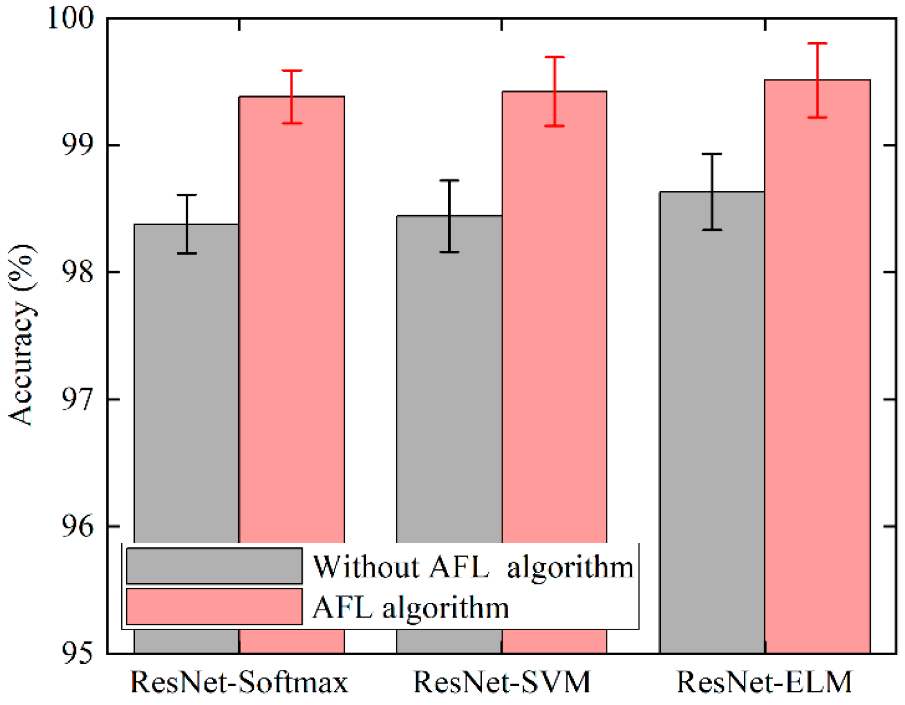
ResNet-Softmax	96.88% ± 0.23	99.22% ± 0.21	97.07% ± 0.22	98.43% ± 0.24
ResNet-SVM	98.44% ± 0.28	99.41% ± 0.21	96.77% ± 0.18	97.11% ± 0.23
ResNet-ELM	98.63% ± 0.31	99.60% ± 0.29	98.79% ± 0.28	99.20% ± 0.21

, with a more intuitive performance comparison shown in Figure 13.

According to the comparison of the data in Table 6, we can know that the average accuracy of the ResNet-Softmax model is 96.88%, which is the lowest accuracy among all models, and the ResNet-SVM and ResNet-ELM are improved by 1.56% and 1.75% relative to ResNet-Softmax. However, the standard deviation of the accuracy of the other two models is also relatively small, and the models are relatively stable. Table 5 also shows that AFL-ResNet-Softmax has a 2.34% improvement compared to ResNet-Softmax, indicating the effectiveness of AFL in improving model performance. Compared with the ResNet-SVM and ResNet-ELM models, the AFL-ResNet-ELM model also improved by nearly 1%. Finally, by comparing the above six models, it can be seen that the excellent performance of the AFL-ResNet-ELM model is visible, which proves the effectiveness of the proposed method and the role of AFL in dealing with the problem of unbalanced data, and, similarly, the excellent performance of the AFL-ResNet-ELM model is obtained from the results of the second evaluation index F₂-score.

In order to better understand the effect of the above models on the check valve dataset, the diagnostic results of each method are visualized through the confusion matrix, as shown in Figure 14.

As the complexity of the model increases, the diagnostic time of the data samples also increases, as shown in

Table 7. Diagnosis time of different classifiers and AFL on the dataset.

Methods	Diagnostic Time/s
	Without AFL	AFL
ResNet-Softmax	0.4830	0.4312
ResNet-SVM	0.7651	0.7120
ResNet-ELM	0.6349	0.6034

. From Table 7, we can clearly draw the following conclusions: when the simple softmax is used as the classifier, the time is better than that of the method in this paper, but it comes at the expense of diagnostic accuracy. However, when the complex ELM is used as the classifier, it can be clearly seen that although the diagnosis time will be slightly worse, the accuracy is within the ideal range, which proves that the proposed method has strong stability. From Figure 14, it can be observed that the overall accuracy of softmax is lower compared to that of the ELM and the SVM, with a significant gap in accurate label recognition. Comparing Figure 14a–f, it is evident that the AFL function outperforms the CE loss function.

To further explore the role of the AFL function in the proposed model, t-SNE was used to visualize the output of the Layer 1 residual module, Layer 5 residual module, the final output of the ResNet module, and the dimensionality reduction output of the ELM for both the ResNet-ELM and AFL-ResNet-ELM models, as shown in Figure 15a–i.

Figure 15 demonstrates that the AFL-ResNet-ELM can distinctly identify different characteristics of check valves, compared to the ResNet-ELM. The AFL-ResNet-ELM classification boundary is more separable than that of the ResNet-ELM, and the AFL-ResNet-ELM model exhibits better training performance at the initial layer. The stronger separability of the AFL-ResNet-ELM indicates the AFL function’s effectiveness, and the AFL-ResNet-ELM accurately identifies the operational state characteristics of the check valve, addressing the monitoring issues of the diaphragm pump’s check valve operation to a significant extent.

5. Conclusions

This paper presents a novel approach for the fast and accurate automatic fault diagnosis of electric check valves by combining the ResNet and ELM models, addressing the need for automatic and high-precision fault diagnosis. Firstly, the grayscale visualization of the original vibration data, along with the integration of the ResNet and ELM, was utilized to effectively extract signal features. In the check valve fault diagnosis dataset, the recognition accuracy of the ResNet-ELM model was improved by 1.75% and 0.19% compared to the ResNet-Softmax and ResNet-SVM models, respectively. Secondly, during the training process, the AFL function was employed instead of the CE function to address data imbalance. The recognition accuracy of the AFL-ResNet-ELM, AFL-ResNet-SVM, and AFL-ResNet-Softmax models was significantly enhanced compared to their non-AFL counterparts, with the ResNet-Softmax model showing a 2.34% improvement in recognition accuracy. Finally, the proposed method provides a practical and accurate solution for monitoring the operational status of check valves, contributing significantly to the health management of check valves, which are crucial components of mineral pipelines. This approach not only meets practical requirements but also enhances fault diagnosis accuracy.

However, there are some limitations in the research presented in this paper. This paper only carries out fault diagnosis on the basis of offline datasets, and the current check valve fault diagnosis model only considers the prediction effect under the experimental data set and filters out the “noise” signal caused by the time-varying characteristics of the slurry medium. If the interference signal in the actual fault diagnosis process is considered, the diagnosis accuracy may be significantly reduced, so in view of the above problems, the author suggests that future research can be carried out in the following directions:

(1)

In the future, data analysis and other means can be used to automatically isolate the interference of “noise” signals, so as to improve the accuracy of diagnosis.

(2)

Only one method is used to solve the problem of data imbalance in this paper, and a variety of methods (data augmentation/resampling) can be used for verification in subsequent studies.

(3)

Future data-driven fault diagnosis algorithms should be based on online system testing rather than offline datasets. Fault diagnosis research should be aimed at practical and online monitoring.

References

- Mu, Z.; Huang, G.; Wu, J.; Fan, Y. Early Fault Diagnosis of Check Valve of High-pressure Diaphragm Pump Based on DEMM. Vibration. Test. Diagn. 2018, 38, 758–764+873. [Google Scholar]
- Hou, C.J.; Ma, J.; Wu, J.D. Research on fault diagnosis of check valve based on CEEMD compound screening and improved SECPSO. J. Comput. 2019, 30, 128–144. [Google Scholar]
- Yuan, J.; Han, T.; Tang, J.; An, L. Intelligent fault diagnosis method for rolling bearings based on wavelet time-frequency diagram and CNN. Mech. Des. Res. 2017, 33, 93–97. [Google Scholar] [CrossRef]
- Huang, H.; Huang, X.; Ding, W.; Yang, M.; Yu, X.; Pang, J. Vehicle vibro-acoustical comfort optimization using a multi-objective interval analysis method. Expert Syst. Appl. 2023, 213, 119001. [Google Scholar] [CrossRef]
- Zhang, C.; Zhang, C.; Guo, X. Research on fault diagnosis of rolling bearing based on MCKD-EWT. Bearing 2020, 5, 43–48. [Google Scholar] [CrossRef]
- Zhou, C.; Ma, J.; Wu, J. Fault Diagnosis of Check Valve Based on CEEMD Compound Screening, BSE and FCM. IFAC-Pap. OnLine 2018, 51, 323–328. [Google Scholar] [CrossRef]
- Pan, Z.; Huang, G.; Fan, Y. A Check Valve Fault Diagnosis Method Based on Variational Mode Decomposition and Permutation Entropy. In Proceedings of the 2019 IEEE 8th Data Driven Control and Learning Systems Conference (DDCLS), Dali, China, 24–27 May 2019; pp. 650–655. [Google Scholar] [CrossRef]
- Chen, Y.; Huang, G.; Feng, Z. Early Fault Diagnosis of High Pressure Diaphragm Pump Check Valve Based on VMD-HMM. In Proceedings of the 2019 IEEE 8th Data Driven Control and Learning Systems Conference (DDCLS), Dali, China, 24–27 May 2019; pp. 808–813. [Google Scholar] [CrossRef]
- Zhao, N.; Zhang, J.; Ma, W.; Jiang, Z.; Mao, Z. Variational time-domain decomposition of reciprocating machine multi-impact vibration signals. Mech. Syst. Signal Process. 2022, 172, 108977. [Google Scholar] [CrossRef]
- Xia, S.; Xia, Y.; Wang, J. Piston Wear Detection and Feature Selection Based on Vibration Signals Using the Improved Spare Support Vector Machine for Axial Piston Pumps. Materials 2022, 15, 8504. [Google Scholar] [CrossRef] [PubMed]
- Wasim, Z.; Zahoor, A.; Muhammad, F.; Niamat, U.; Kim, K. Centrifugal Pump Fault Diagnosis Based on a Novel SobelEdge Scalogram and CNN. Sensors 2023, 23, 5255. [Google Scholar] [CrossRef] [PubMed]
- Ma, M.; Sun, C.; Zhang, C.; Chen, X. Subspace-based MVE for performance degradation assessment of aero-engine bearings with multimodal features. Mech. Syst. Signal Process. 2019, 124, 298–312. [Google Scholar] [CrossRef]
- Huang, H.; Lim, T.C.; Wu, J.; Ding, W.; Pang, J. Multitarget prediction and optimization of pure electric vehicle tire/road airborne noise sound quality based on a knowledge-and data-driven method. Mech. Syst. Signal Process. 2023, 197, 110361. [Google Scholar] [CrossRef]
- Li, K.; Gao, X.; Tian, Z.; Qiu, Z. Using the curve moment and the PSO-SVM method to diagnose downhole conditions of a sucker rod pumping unit. Pet. Sci. 2013, 10, 73–80. [Google Scholar] [CrossRef]
- Li, R.; Fan, Y. Fault Diagnosis of Check Valve of High-pressure Diaphragm Pump Based on CEEMDAN Multi-scale Arrangement Entropy and SO-RELM. Vib. Shock 2023, 42, 127–135. [Google Scholar]
- Ma, J.; Wu, J.; Wang, X. Fault Diagnosis Method of Check Valve Based on Multikernel Cost-Sensitive Extreme Learning Machine. Complexity 2017, 2017, 8395252. [Google Scholar] [CrossRef]
- Xu, W.H.; Fu, K. An intelligent diagnostic system for reciprocating machine. In Proceedings of the 1997 IEEE International Conference on Intelligent Processing Systems, Beijing, China, 28–31 October 1997; pp. 1520–1522. [Google Scholar] [CrossRef]
- Chen, Z.; Mauricio, A.; Li, W.; Gryllias, K. A deep learning method for bearing fault diagnosis based on Cyclic Spectral Coherence and Convolutional Neural Networks. Mech. Syst. Signal Process. 2020, 140, 106683. [Google Scholar] [CrossRef]
- Bie, F.; Du, T.; Lyu, F. An integrated approach based on improved CEEMDAN and LSTM deep learning neural network for fault diagnosis of reciprocating pump. IEEE Access 2021, 9, 23301–23310. [Google Scholar] [CrossRef]
- Wei, X.L.; Chao, Q.; Tao, J.F. Cavitation fault diagnosis method for high-speed plunger pumps based on LSTM and CNN. Acta Aeronaut. Astronaut. Sin. 2021, 42, 423876. [Google Scholar] [CrossRef]
- Chen, Z.; Chen, S.; Chen, X.; Li, C.; Sanchez, R.V.; Qin, H. Deep neural networks-based rolling bearing fault diagnosis. Microelectron. Reliab. 2017, 75, 327–333. [Google Scholar] [CrossRef]
- Li, G.; Hu, J.; Shan, D.; Ao, J.; Huang, B.; Huang, Z. A CNN model based on innovative expansion operation improving the fault diagnosis accuracy of drilling pump fluid end. Mech. Syst. Signal Process. 2023, 187, 109974. [Google Scholar] [CrossRef]
- Tamilselvan, P.; Wang, P. Failure diagnosis using deep belief learning based health state classification. Reliab. Eng. Syst. Saf. 2013, 115, 124–135. [Google Scholar] [CrossRef]
- Muhammad, F.; Zahoor, A.; Kim, J. Pipeline leak diagnosis based on leak-augmented scalograms and deep learning. Eng. Appl. Comput. Fluid Mech. 2023, 17, 1. [Google Scholar] [CrossRef]
- Prosvirin, A.; Ahmad, Z.; Kim, J. Global and Local Feature Extraction Using a Convolutional Autoencoder and Neural Networks for Diagnosing Centrifugal Pump Mechanical Faults. IEEE Access 2021, 9, 65838–65854. [Google Scholar] [CrossRef]
- Mao, W.; He, L.; Yan, L.; Wang, J. Online sequential prediction of bearings imbalanced fault diagnosis by extreme learning machine. Mech. Syst. Signal Process. 2017, 83, 450–473. [Google Scholar] [CrossRef]
- Huang, H.; Wu, J.; Lim, T.; Yang, M.; Ding, W. Pure electric vehicle nonstationary interior sound quality prediction based on deep CNNs with an adaptable learning rate tree. Mech. Syst. Signal Process. 2021, 148, 107170. [Google Scholar] [CrossRef]
- Tang, Y.; Zhang, Y.Q.; Chawla, N.V.; Krasser, S. SVMs modeling for highly imbalanced classification. IEEE Trans. Syst. Man Cybern. 2009, 9, 281–288. [Google Scholar] [CrossRef]
- Haixiang, G.; Yijing, L.i.; Shang, J.; Mingyun, G.u.; Yuanyue, H.; Bing, G. Learning from class-imbalanced data: Review of methods and applications. Exp. Syst. Appl. 2017, 73, 220–239. [Google Scholar] [CrossRef]
- Zhang, C.; Tan, K.C.; Li, H.; Hong, G.S. A cost-sensitive deep belief network for imbalanced classification. IEEE Trans. Neural Netw. Learn. Syst. 2019, 30, 109–122. [Google Scholar] [CrossRef]
- Chawla, V.; Nitesh, W.; Kevin, W.; Bowyer, O.; Lawrence, W.; Kegelmeyer, W.P. SMOTE: Synthetic minority over-sampling technique. Artif. Intell. 2002, 16, 321–357. [Google Scholar] [CrossRef]
- Douzas, G.; Bacao, F.; Last, F. Improving imbalanced learning through a heuristicoversampling method based on k-means and SMOTE. Inf. Sci. 2018, 456, 1–20. [Google Scholar] [CrossRef]
- Qian, M.; Li, Y. A weakly supervised learning-based oversampling framework for classimbalanced fault diagnosis. LEEE Trans. Reliab. 2022, 71, 429–442. [Google Scholar] [CrossRef]
- Qin, Z.; Yu, D.; Chen, L.; Chao, W.; Liang, M.; Tao, L.; Ma, J. An adaptive fault diagnosis framework under class-imbalanced conditions based on contrastive augmented deep reinforcement learning. Expert Systems with Applications. 2023, 234, 121001. [Google Scholar] [CrossRef]
- Lin, T.; Goyal, P.; Girshick, R. Focal loss for dense object detection. IEEE Trans. Pattern Anal. Mach. Intell. 2020, 42, 318–327. [Google Scholar] [CrossRef] [PubMed]
- Zhou, W.; Li, X.; Yi, J. A novel UKF-RBF method based on adaptive noise factor for fault diagnosis in pumping unit. IEEE Trans. Ind. Inform. 2019, 15, 1415–1424. [Google Scholar] [CrossRef]
- Li, C.; Sanchez, R.; Zurita, G.; Cerrada, V.; Cabrera, D.; Vasquez, R. Multimodal deep support vector classification with homologous features and its application to gearbox fault diagnosis. Neurocomputing 2015, 168, 119–127. [Google Scholar] [CrossRef]
- Wang, B.; Guo, J.; Zhang, Y. Application of learning receptive field algorithm based on deep networkin image classification. Control Theory Appl. 2015, 32, 1114–1119. [Google Scholar] [CrossRef]
- Jia, F.; Lei, Y.; Lin, J.; Zhou, X.; Lu, N. Deep neural networks:a promising tool forfault characteristic mining and intelligent diagnosis of rotating machinerywith massive data. Mech. Syst. Signal Process. 2016, 7273, 303–315. [Google Scholar] [CrossRef]
- Huang, H.; Huang, X.; Ding, W.; Zhang, S.; Pang, J. Optimization of electric vehicle sound package based on LSTM with an adaptive learning rate forest and multiple-level multiple-object method. Mech. Syst. Signal Process. 2023, 187, 109932. [Google Scholar] [CrossRef]
- Douzas, G.; Bacao, F. Effective data generation for imbalanced learning using conditional generative adversarial networks. Exp. Syst. 2018, 91, 464–471. [Google Scholar] [CrossRef]
- Malik, J.; Mishra, S. Proximal support vector machine (PSVM) based imbalance fault diagnosis of wind turbine using generator current signals. Energy Proc. 2016, 90, 593–603. [Google Scholar] [CrossRef]
- Sun, P.; Dai, R.; Li, H.; Zheng, Z.; Wu, Y.; Huang, H. Multi-Objective Prediction of the Sound Insulation Performance of a Vehicle Body System Using Multiple Kernel Learning–Support Vector Regression. Electronics 2024, 13, 538. [Google Scholar] [CrossRef]
- Jiao, J.; Zhao, M.; Lin, J.; Ding, C. Deep coupled dense convolutional network with complementary data for intelligent fault diagnosis. IEEE Trans. Ind. Electron. 2019, 66, 9858–9867. [Google Scholar] [CrossRef]
- Huang, H.; Huang, X.; Li, R.; Lim, T.; Ding, W. Sound quality prediction of vehicle interior noise using deep belief networks. Applied Acoustics. 2016, 113, 149–161. [Google Scholar] [CrossRef]
- He, K.; Zhang, X.; Ren, S.; Sun, J. Deep Residual Learning for Image Recognition. arXiv 2015, arXiv:1512.03385. [Google Scholar] [CrossRef]
- Huang, G.; Zhu, Q.; Siew, C. Extreme learning machine: A new learning scheme of feedforward neural networks. In Proceedings of the 2004 IEEE International Joint Conference on Neural Networks, Budapest, Hungary, 25–29 July 2004; pp. 985–990. [Google Scholar]
- He, K.; Zhang, X.; Ren, S.; Sun, J. Identity Mappings in Deep Residual Networks; Lecture Notes in Computer Science; Springer: Cham, Switzerland, 2016; pp. 630–645. [Google Scholar] [CrossRef]
- Huang, G.; Zhu, Q.; Siew, C. Extreme learning machine: Theory and applications. Neurocomputing 2006, 70, 489–501. [Google Scholar] [CrossRef]
- Wu, Y.; Liu, X.; Huang, H.; Wu, Y.; Ding, W. Multi-Objective Prediction and Optimization of Vehicle Acoustic Package Based on ResNet Neural Network. Sound Vib. 2023, 57, 73–95. [Google Scholar] [CrossRef]
- Zhao, H.; Wang, J.; Lee, J.; Li, Y. A compound interpolation envelope local mean decomposition and its application for fault diagnosis of reciprocating compressors. Mech. Syst. Signal Process. 2018, 110, 273–295. [Google Scholar] [CrossRef]
- Fröhlingsdorf, K.; Dreßen, M.; Pischinger, S.; Steffens, C. Analysis of the Influence of Image Processing, Feature Selection, and Decision Tree Classification on Noise Separation of Electric Vehicle Powertrains. SAE Int. J. Veh. Dyn. Stab. NVH 2023, 7, 23–33. [Google Scholar] [CrossRef]
- Li, X.; Lv, C.; Wang, W.; Li, G.; Yang, L.; Yang, J. Generalized Focal Loss: Towards Efficient Representation Learning for Dense Object Detection. IEEE Trans Pattern Anal Mach Intell. 2023, 3139–3153. [Google Scholar] [CrossRef]
- Chong, U. Signal model-based fault detection and diagnosis for induction motors using features of vibration signal in two-dimension domain. Stroj. Vestn. Mech. Eng. 2011, 57, 655–666. [Google Scholar] [CrossRef]
- Liu, Z.; Li, S.; Wang, R.; Jia, X. Research on Fault Feature Extraction Method of Rolling Bearing Based on SSA–VMD–MCKD. Electronics 2022, 11, 3404. [Google Scholar] [CrossRef]
- Huang, H.; Li, R.X.; Yang, M.L.; Lim, T.C.; Ding, W. Evaluation of vehicle interior sound quality using a continuous restricted Boltzmann machine-based DBN. Mech. Syst. Signal Process. 2017, 84, 245–267. [Google Scholar] [CrossRef]
- Xu, Q.; Lu, S.; Jia, W.; Jiang, C. Imbalanced fault diagnosis of rotating machinery via multi-domain feature extraction and cost-sensitive learning. Intell. Manuf. 2020, 31, 1467–1481. [Google Scholar] [CrossRef]
- Yuan, W.; Yang, Q. A Novel Method for Pavement Transverse Crack Detection Based on 2D Reconstruction of Vehicle Vibration Signal. KSCE J. Civ. Eng. 2023, 27, 2868–2881. [Google Scholar] [CrossRef]