Dynamic Current-Limitation Strategy of Grid-Forming Inverters Based on SR Latches

Abstract

A grid-forming (GFM) inverter can effectively support active power and reactive power, and the stability problem induced by the low inertia can be thereby alleviated in a power electronics-dominated power system. Yet, the voltage source characteristic presented by the grid-forming inverter induces an overcurrent problem during a short-circuit fault. Furthermore, the time delay induces an inrush current in traditional digital control, triggered by a predefined timing sequence. To address the overcurrent problem of the GFM inverter controlled by the digital controller, the operation characteristics of GFM inverters under grid-voltage drops are investigated, and a mathematical model of the instantaneous fault current is established, which depicts the relationship between the instantaneous fault current’s magnitude, grid-voltage drop severity, equivalent output impedance, and current inner-loop response speed. Then, a Set–Reset (SR) latch-based dynamic current limitation with event-triggered control is proposed for the low-voltage ride-through of the GFM inverter. In the proposed method, the current limitation is enabled during grid fault, and the active and reactive powers can be recovered rapidly after fault clearance. Meanwhile, the active and reactive power references are designed to enhance synchronization stability during the grid fault. The proposed method addresses the issue of the repeated switching of virtual impedance during grid fault and achieves rapid power recovery after fault clearance. In addition, the proposed method uses the logic of event triggers to respond to the overcurrent event in real time and realize overcurrent protection. The simulation and experimental results demonstrate the effectiveness of the proposed method in current limitation and active-power recovery after fault clearance.

1. Introduction

In recent years, renewable energy generation, such as solar and wind power generation, has grown rapidly. However, as the proportion of the traditional synchronous generators decreases, low inertia induces stability issues in power electronics-dominated power systems [1,2].

Currently, a grid-following (GFL) control is usually applied for the regulation of the grid current of a grid-connected inverter. Although the active and reactive power can be controlled independently, the GFL control presents a lack of rotational inertia similar to traditional synchronous generators [3]. Consequently, power systems characterized by a high proportion of renewable energy sources and power electronic devices tend to have low inertia and damping, and the voltage and frequency stability thereby are affected by the increase in the power-electronic devices [4]. Additionally, the traditional grid-following inverter suffers from issues, such as synchronization instability in weak grids. Hence, to mitigate frequency and voltage fluctuations in power systems and enhance system stability for renewable-energy power systems, a grid-forming (GFM) control has been proposed by some of the literature [5,6,7]. The typical GFM control methods include the droop control [8], droop control with pre-filter [9,10], virtual synchronous machine control [11,12], power synchronization control [13], and virtual oscillator control [14].

The GFM inverter is similar to the controlled voltage source illustrated in Figure 1. The collected PCC point voltage v_pcc and current i_pcc generate the reference voltage V_m and phase θ of the inner loop through the power control loop. However, typical GFM inverters maintain a constant internal potential even in grid voltage sag, and overcurrent issues thereby are introduced by GFM control during voltage sag. Therefore, the overcurrent protection scheme should be analyzed during grid voltage sag. Furthermore, the rapid recovery of active power is necessary after fault clearance. Numerous studies have proposed current-limitation strategies for GFM inverters during grid faults.

To address the issue of overcurrent in GFM inverters during grid-voltage drop, power electronic devices can be designed with higher power ratings to withstand larger current surges. However, this approach inevitably increases the cost of the inverter. One current-limitation method is the restriction of the current loop to limit the current amplitude [15,16,17,18]. Nonetheless, this method may lead to the saturation of the voltage outer loop; the voltage-control loop thereby would hardly be recovered after fault clearance, and the stable operation of the inverter could not be guaranteed and even suffer from transient instability issues [18]. Additionally, the output current can be limited by restricting inverter output power [19]. Yet, the dynamic response of the current limitation is ignored.

Moreover, a virtual impedance-based current-limitation method is proposed, which modifies the reference of the voltage loop and reduces the output current reference of the voltage controller [20,21,22,23,24,25]. In [21], the method based on virtual impedance can effectively suppress the fault current and oscillation in the process of power-grid-fault recovery. In [22], a small signal-modeling and controller parameter-tuning method based on adaptive virtual impedance for current limitation is proposed. In [23], a mathematical model of VSG with virtual resistance is presented. On this basis, the transient stability of the nonlinear system is analyzed using the phase diagram and the attractive region of the nonlinear system. In [24], the transient synchronization instability, which is induced by the over-limitation of the power transmission, is analyzed and suppressed by dynamic current-limitation control. In [25], the relationship between the virtual resistance and transient overcurrent is elaborated, and the transient overcurrent suppression method is proposed by introducing virtual resistance during symmetrical faults, where the larger virtual resistance leads to smaller transient currents.

In addition, adjusting PCC point voltage can also limit the output current [26,27]. However, when interference occurs, the inverter terminal voltage must be dropped to reduce the inverter-phase current amplitude. Therefore, the voltage controller has a saturation problem. In order to solve such a problem, anti-saturation algorithms can be designed. In [28], when the current limiter is triggered, the integrator of the voltage controller is set to zero to improve the fault-recovery capability of the GFM inverter. In [29,30], the outer loop controller was redesigned as a priority-based current limiter to avoid the saturation of the voltage controller. However, these methods are only suitable for specific inner-loop and outer-loop control structures and system parameters. Once the control structure or system parameters change, these methods lose their effectiveness.

The above different current-limitation methods are summarized in

Table 1. Current-limitation method.

Current-Limitation Method	Advantage	Defect
High-power device	Strong overcurrent ability	High cost
Current loop limitation [15,16,17,18]	Simple design and control	Voltage loop saturation, may fail to restore [18]
Output power limitation	Avoid voltage loop saturation	Ignore dynamic response
Virtual impedance [20,21,22,23,24,25]	Avoid voltage loop saturation, good to restore	Difficulty in switching
Voltage loop limitation [26,27]	Good to restore	Anti-saturation algorithm complexity, low applicability [28,29,30]

.

However, the aforementioned methods fail to address the issue of the overcurrent caused by a time trigger. Therefore, droop control with dynamic current limitation based on Set-Reset (SR) latch event-triggered logic is proposed for current limitation. This approach not only effectively addresses the problem of virtual impedance toggling caused by variations in the grid current, but also facilitates current limitation during grid fault and rapid power recovery after fault clearance. The contributions of this paper are as follows:

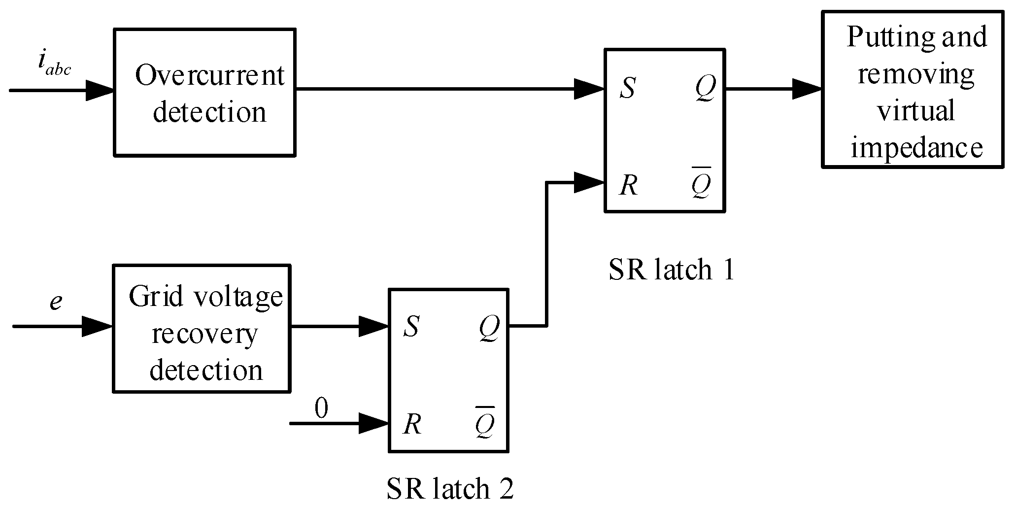
• The proposed dynamic current-limitation strategy based on SR latch logic not only suppresses transient overcurrents during grid-voltage drops but also effectively addresses the issue of irregular toggling of virtual impedance. Furthermore, it enables rapid power recovery after fault clearance.
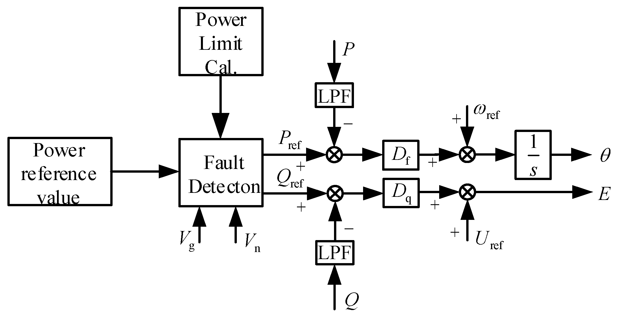
• The virtual-impedance method with power reference regulation based on grid codes is proposed for enhancing transient synchronization stability, and transient synchronization instability is effectively avoided under grid fault. The inverter reaches a new operating point quickly after the grid fault, and the dynamic performance is improved effectively.
• The proposed method is similar to the hardware SR latch, which has high speed and is not affected by time-triggered interruptions. Therefore, both the real-time triggering of SR hardware and the flexibility of digital controllers are taken into account, and the inverter control and fast overcurrent protection can be realized by digital control.

In this study, an SR latch is proposed to achieve the above logic, as shown in Figure 2, and the truth table is shown in

Table 2. SR latch truth table.

S	R	State
1	0	1
0	1	0
0	0	hold

. When an overcurrent is detected, S = 1 and R = 0 for the SR latch 1 and a high-level output will activate the virtual impedance. After the virtual impedance activation, S = 0 and R = 0 for the SR latch 1 and a high-level output should be held.

The SR latch 2 output in the grid recovery detection section is low during grid fault. The grid recovery detection outputs a high-level signal when the grid fault recovers, and the Q of SR latch 2 is equal to the R of SR latch 1. Therefore, the R of SR latch 1, which enables/disables the virtual impedance, will be at a high-level during fault recovery and will mean removing the virtual impedance.

In practice, overcurrent detection adopts high-speed sampling, which directly triggers the protection logic after detecting the overcurrent, and does not trigger according to the timing. That is, the control logic triggers the interruption on time, and the protection logic triggers the interruption on event.

2. Mathematical Model of Grid-Forming Inverters

2.1. System Description

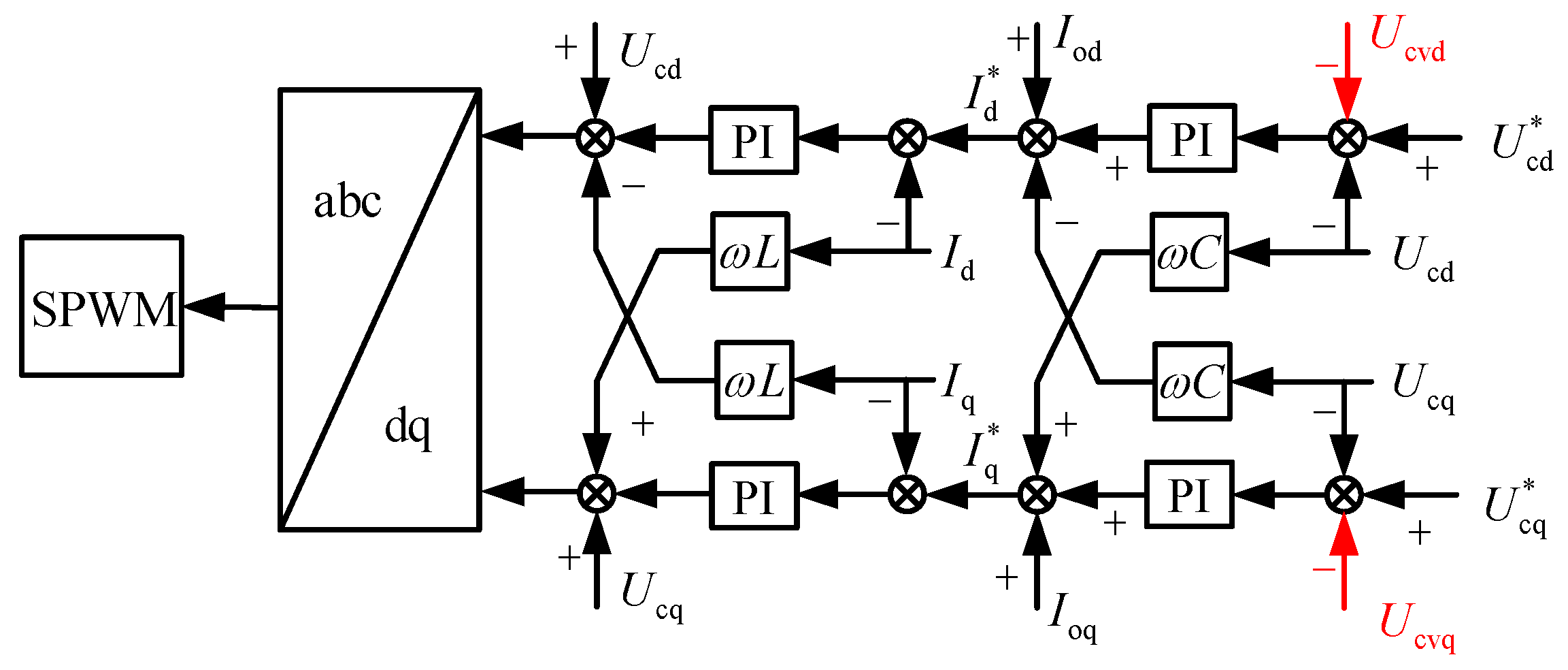
The topology and control system of the grid-connected inverter are illustrated in Figure 3. Here, u_dc represents the DC-side voltage of the inverter, which is typically supplied by photovoltaic or wind power sources; C_dc represents the DC-side capacitor. The high-frequency harmonics on the AC side of the inverter are filtered out by the LC filter. The inverter is connected to the point of common coupling (PCC), and the grid-side equivalent inductance is represented as L_g.

The control system of the GFM inverter, as illustrated in Figure 3, shows that the control system includes the power calculation, power control loop, voltage and current-control loop, and modulation. The voltage and current at the PCC are measured to calculate the active and reactive power. The voltage vector reference is determined by the power control loop. A voltage-current dual-loop control scheme is applied to calculate the modulating voltage, and the sinusoidal pulse width modulation (SPWM) is applied to generate switching drive signals.

2.2. Power Control

The equivalent circuit and vector representation of the GFM inverter are illustrated in Figure 4. V represents the magnitude of the GFM inverter output voltage. I is the magnitude of the GFM inverter output current. φ indicates the phase difference between the output voltage and current of the GFM inverter. E represents the magnitude of the grid voltage. δ is the phase difference between the output voltage of the GFM inverter and the grid voltage. R and X represent the equivalent output resistance and reactance, respectively.

The active power and reactive power of the GFM inverter are expressed by (1).

$$\left\{\begin{array}{l}P={\displaystyle \frac{V}{R^2+X^2}}\left[R(V-E\cos \delta )+XE\sin \delta \right]\\ Q={\displaystyle \frac{V}{R^2+X^2}}\left[X(V-E\cos \delta )-RE\sin \delta \right]\end{array}\right.$$

(1)

The line resistor is relatively low (X≫R); therefore, only line inductance needs to be considered. The phase difference δ between the output voltage of the GFM inverter and the grid voltage is usually small, and it can be assumed that sin δ = δ, cos δ = 1 [31]. Therefore, (1) can be simplified as

$$\left\{\begin{array}{l}P={\displaystyle \frac{V}{X}}E\delta \\ Q={\displaystyle \frac{V}{X}}(V-E)\end{array}\right.$$

(2)

The positive correlation, which is expressed in (2), between the active power P and power angle δ indicates that active power can be used to regulate the output voltage angle of the inverter, and the voltage angle can be adjusted by angle frequency ω. Similarly, reactive power Q can be used to regulate the output voltage of the inverter. Therefore, the power control loop, which calculates the desired voltage and angle frequency, can be expressed as follows [6,32]:

$$\left\{\begin{array}{l}\theta ={\displaystyle \frac{1}{s}}[{\omega }_{\mathrm{ref}}+D_{\mathrm{f}}(P^{*}-P)]\\ U=U_{\mathrm{ref}}+D_{\mathrm{q}}(Q^{*}-Q)\end{array}\right.$$

(3)

where ω_ref and U_ref are the reference for the grid frequency and voltage, respectively. D_f and D_q are the droop-controlled coefficients for the active and reactive power, respectively. P^* and Q^* represent the active and reactive power references of the GFM inverter, respectively. P and Q are the active and reactive power of the GFM inverter, respectively. Finally, 1/s is the Laplace transformation of the integral.

The low-pass filter (LPF) usually is used for power-ripple suppression and providing virtual inertia for system frequency stability in the droop-controlled loop. The LPF not only filters out high-order harmonics but also prevents interactions between the droop controller and voltage- and current-control loops [33]. The transfer function of the LPF is represented by (4), and the block diagram of the droop control with the low-pass filter is depicted in Figure 5. The reference voltage phase θ and amplitude E are calculated from the active droop loop and reactive droop loop.

$$\mathrm{LPF}={\displaystyle \frac{{\omega }_{\mathrm{c}}}{s+{\omega }_{\mathrm{c}}}}={\displaystyle \frac{1}{1+T_{\mathrm{f}}s}}$$

(4)

where ω_c represents the cutoff angular frequency and T_f represents the time constant.

The active power control loop depicted in Figure 5 can be expressed as

$$P^{*}-{\displaystyle \frac{1}{1+T_{\mathrm{f}}s}}P={\displaystyle \frac{1}{D_{\mathrm{f}}}}(\omega -{\omega }_{\mathrm{ref}})$$

(5)

Equation (5) can be rewritten as

$$\begin{array}{l}P=(1+T_{\mathrm{f}}s)\left[{\displaystyle \frac{1}{D_{\mathrm{f}}}}({\omega }_{\mathrm{ref}}-\omega )+P^{*}\right]\\ ={\displaystyle \frac{{\omega }_{\mathrm{ref}}-\omega }{D_{\mathrm{f}}}}+{\displaystyle \frac{T_{\mathrm{f}}s\cdot {\omega }_{\mathrm{ref}}}{D_{\mathrm{f}}}}-\\ {\displaystyle \frac{T_{\mathrm{f}}s\cdot \omega }{D_{\mathrm{f}}}}+P^{*}+T_{\mathrm{f}}s\cdot P^{*}\end{array}$$

(6)

The derivative of the constant is zero in (6), which can be simplified as

$$T_{\mathrm{f}}{\displaystyle \frac{1}{D_{\mathrm{f}}}}s\cdot \omega =P^{*}-P-{\displaystyle \frac{\omega -{\omega }_{\mathrm{ref}}}{D_{\mathrm{f}}}}$$

(7)

Equation (7) can be expressed as (8) in the time–domain expression.

$$T_{\mathrm{f}}{\displaystyle \frac{1}{D_{\mathrm{f}}}}\cdot {\displaystyle \frac{\mathrm{d}\omega }{\mathrm{d}t}}=P^{*}-P-{\displaystyle \frac{\omega -{\omega }_{\mathrm{ref}}}{D_{\mathrm{f}}}}$$

(8)

It can be seen that the droop control with a low-pass filter is equivalent to the virtual synchronous generator control [7].

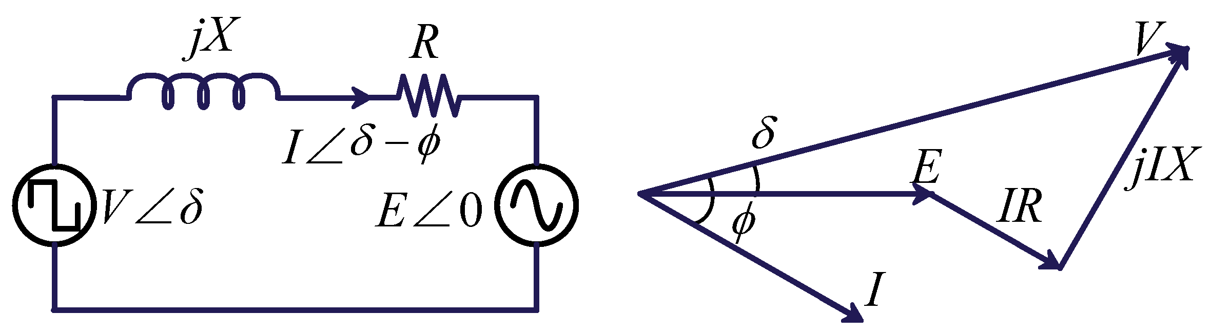
3. GFM Inverter Operation Characteristics under Grid Faults

The equivalent circuit model of the GFM inverter under grid fault is illustrated in Figure 6. Here, V represents the virtual internal potential of the GFM inverter. I is the output current of the GFM inverter. R + jX is the equivalent impedance from the GFM inverter to the fault point. U_p is the fault-point voltage. R′ + jX′ is the line impedance between the fault point and the grid, and E is the grid voltage.

The fault-point voltage variation can be expressed as follows [25]:

$$\mathsf{\Delta }{U}_{\mathrm{p}}=U_{\mathrm{p}}(0_{-})-U_{\mathrm{p}}(0_{+})$$

(9)

where ΔU_p represents the change in the fault-point voltage vector, and where U_p(0₋) and U_p(0₊) denote the fault-point voltage before and after the fault occurrence, respectively.

It is assumed that the internal potential is unchanged during grid voltage sag. In this case, according to Kirchhoff’s voltage law, it can be derived as

$$RI+L{\displaystyle \frac{\mathrm{d}I}{\mathrm{d}t}}=V-U_{\mathrm{p}}$$

(10)

Substituting (9) into (10), the expression for the output current of the GFM inverter during grid-voltage drops can be expressed as

$$\left\{\begin{array}{l}I(t)=I(\infty )+\left[I(0_{+})-{\left.I(\infty )\right|}_{0+}\right]{\mathrm{e}}^{-tR/L}\\ \mathsf{\Delta }I(t)=I(\infty )-{\left.I(\infty )\right|}_{0+}{\mathrm{e}}^{-tR/L}\\ I(\infty )={\displaystyle \frac{V-U_{\mathrm{p}}(0_{+})}{R+jX}}\\ {\left.I(\infty )\right|}_{0+}={\displaystyle \frac{V-U_{\mathrm{p}}(0_{-})}{R+jX}}\end{array}\right.$$

(11)

where I(t) represents the output current, I(0₊) denotes the initial current at the instance of the fault, I(∞) represents the steady-state current after the fault occurrence, and I(∞)∣₀₊ is the value of I(∞) when the fault occurs. ΔI(t) represents the instantaneous fault current. L/R represents the time constant.

Since the droop control with a low-pass filter is equivalent to the virtual synchronous generator (VSG), the internal potential V changes randomly according to the original power instruction. Therefore, the output-current command value has a long transition process. And because the current loop adopts proportional control, the attenuation characteristic of the instantaneous fault current can be ignored. Hence, the instantaneous fault current can be derived from (11) as

$$\mathsf{\Delta }I(t)={\displaystyle \frac{\mathsf{\Delta }{U}_{\mathrm{p}}}{R+jX}}$$

(12)

It can be seen from the above analysis that the line current is impacted by the grid-voltage drop, the equivalent line impedance, and the response speed of the current-control loop. Therefore, the fault current can be suppressed by the increase in the equivalent output impedance and the response speed of the current inner loop. And the equivalent output impedance can be regulated by the virtual impedance.

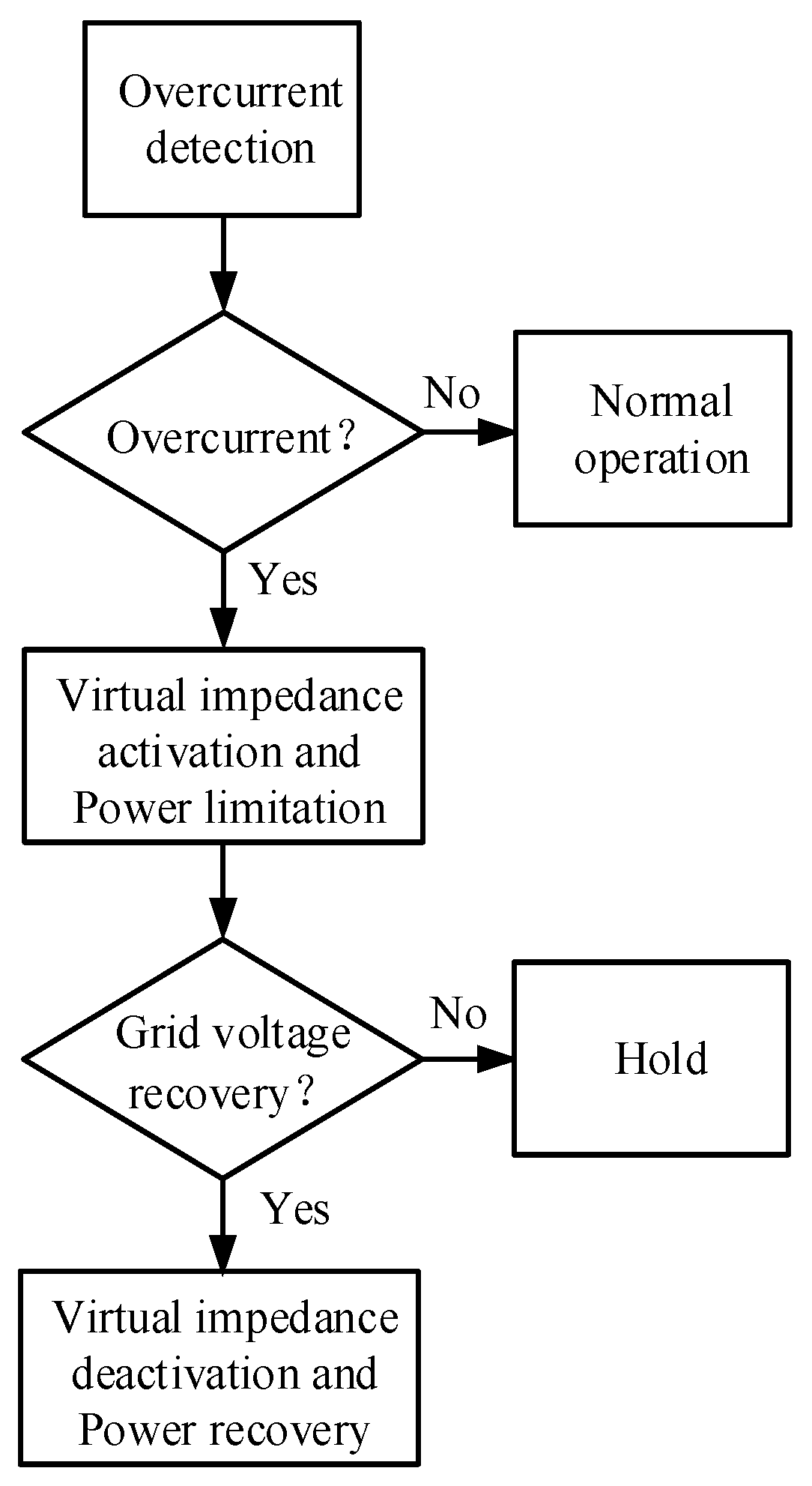
4. Dynamic Current-Limitation Strategy with Virtual Impedance and Power Limitation

According to (12), the expression for fault current with virtual impedance is

$$\mathsf{\Delta }{I}_{\mathrm{v}}(t)={\displaystyle \frac{\mathsf{\Delta }{U}_{\mathrm{p}}}{(R+R_{\mathrm{v}})+j(X+X_{\mathrm{v}})}}$$

(13)

where R_V and X_V represent the virtual resistance and reactance, respectively.

The application of the virtual impedance is described as follows: During normal operation, the virtual impedance is not activated. When the output current exceeds the threshold, the virtual impedance is activated to suppress fault currents. When the grid voltage is recovered, the virtual impedance is deactivated. The output current should be limited to the permissible range, i.e., the amplitude of the output current should be less than 1.3. Thus, the variation in currents caused by grid-voltage drops should be less than 0.3 [25]. Therefore, to retain a certain safety margin, the overcurrent threshold is set to 1.2 in this paper. The virtual impedance is calculated as follows:

$$X_{\mathrm{v}}=(1.2-1)\times I_{\mathrm{n}}{K}_{\mathrm{v}}{\sigma }_{X/R}$$

(14)

where K_V and ${\sigma }_{X/R}$ represent the virtual impedance limiting gain and the ratio of reactance to resistance. I_n represents rated current.

The proposed logic-control block diagram for switching the virtual impedance is depicted in Figure 2. Initially, the three-phase current is detected and compared to the current threshold. When the overcurrent is detected, a high signal level is generated. During the grid fault, once overcurrent is detected, the virtual impedance must remain activated to limit the overcurrent.

However, after virtual impedance activation, the overcurrent detection module cannot detect the overcurrent signal due to the current-limitation characteristic of the virtual impedance, and the overcurrent detection module will output at a low level. Nevertheless, the virtual impedance must remain activated during the grid fault. Therefore, the overcurrent state should be held after virtual impedance activation.

The voltage-current dual-loop control block diagram with virtual impedance is illustrated in Figure 7. Here, U_cvd and U_cvq represent the voltage drops across the virtual impedance, which are computed by (15) [21].

$$\left[\begin{array}{l}{U}_{\mathrm{cvd}}\\ U_{\mathrm{cvq}}\end{array}\right]=\left[\begin{array}{cc}{R}_{\mathrm{v}}& -\omega L_{\mathrm{v}}\\ R_{\mathrm{v}}& \omega L_{\mathrm{v}}\end{array}\right]\left[\begin{array}{l}{i}_{\mathrm{d}}\\ i_{\mathrm{q}}\end{array}\right]$$

(15)

The synchronization stability problem will occur with large line impedance in grid-sag conditions [21], yet the introduction of the virtual impedance increases the equivalent line impedance, and synchronization stability should be considered. In the case of synchronization instability, the power-angle curve (P-δ curve) drops due to severe voltage sag, and there is no intersection between the active power reference and the P-δ curve. Therefore, the current injection should be limited to ensure system stability. Referring to the grid-connection standards of the German Association of Energy and Water Industries (BDEW), the injected reactive power current into the grid should be

$$i_{\mathrm{q}}=i_{\mathrm{q}}(t_{-})+2{\displaystyle \frac{\mathsf{\Delta }U}{U}}{I}_{\mathrm{n}}$$

(16)

where i_q represents the reactive current demand during the grid-voltage drop, while i_q(t₋) is the amplitude of the reactive current before the instance of the grid-voltage drop. I_n represents the rated current.

However, the grid current cannot be directly controlled by the GFM inverter. The reactive power current injection should be controlled indirectly by the output voltage, which is regulated by the active and reactive power. According to (16), the reactive power reference is designed as

$$Q_{\mathrm{ref}}=1.5u_{\mathrm{pd}}{i}_{\mathrm{q}}=1.5u_{\mathrm{pd}}{i}_{\mathrm{q}}(t_{-})+3u_{\mathrm{pd}}{\displaystyle \frac{\mathsf{\Delta }U}{U}}{I}_{\mathrm{n}}$$

(17)

where Q_ref represents the reactive power reference, while u_pd is the d-axis component of the grid voltage.

According to the grid codes, the magnitude of the active current is limited by the reactive current, as expressed in (18). When the reactive current reference exceeds the rated current, the active current or active power reference is set to zero.

$$\left\{\begin{array}{l}{i}_{\mathrm{d}}\le \sqrt{I_{\mathrm{n}}^2-i_{\mathrm{q}}^2}\\ P_{\mathrm{ref}}=1.5u_{\mathrm{pd}}{i}_{\mathrm{d}}\end{array}\right.$$

(18)

where i_d is the active current, and P_ref is the active power reference.

The power modification for the dynamic current-limiting of GFM inverters based on droop control with LPF is illustrated in Figure 8. After detecting a grid-voltage drop, the reference power of the GFM inverter is recalculated by (17)–(18), and the modified active and reactive power can ensure system stability and effectively limit the output-current magnitude. After fault clearance, the active and reactive power references are recovered to their original value. Furthermore, since both the virtual impedance and power limitation dynamically restrict the fault current, the GFM inverter ultimately achieves low-voltage ride-through and no overcurrent during faults and fault recovery, and the maximum injection of reactive power is achieved for system stability.

The implementation flow chart of dynamic current limitation is shown in Figure 9. When the inverter detects the output current overcurrent, it immediately enables the virtual impedance and limits the power; otherwise, it runs normally. When the grid voltage recovery is detected, the virtual impedance is immediately removed and the original power is restored; otherwise, the operation continues.

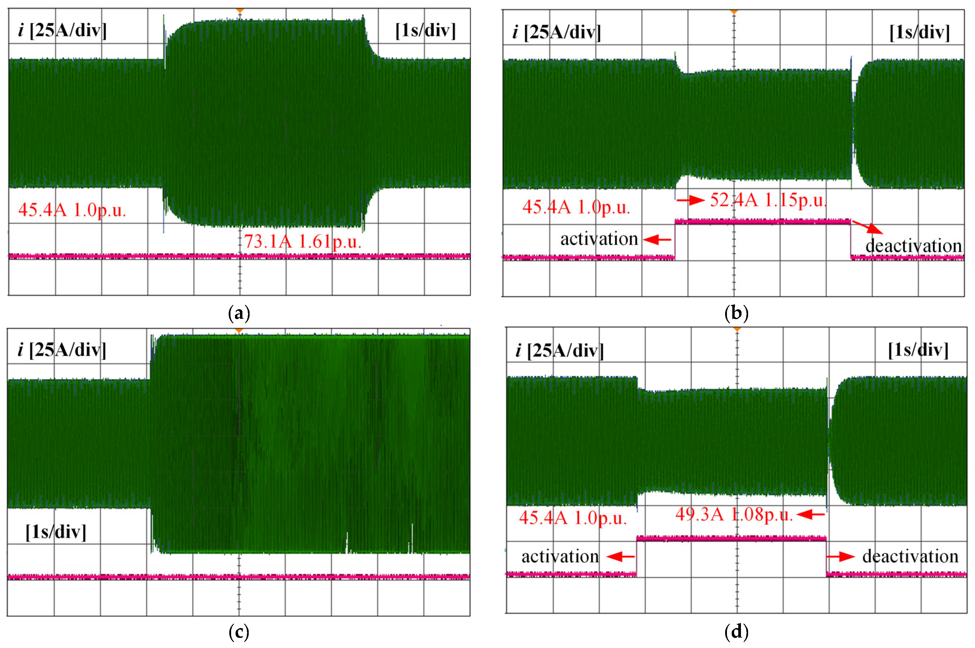
5. Simulation and Experiment Verification

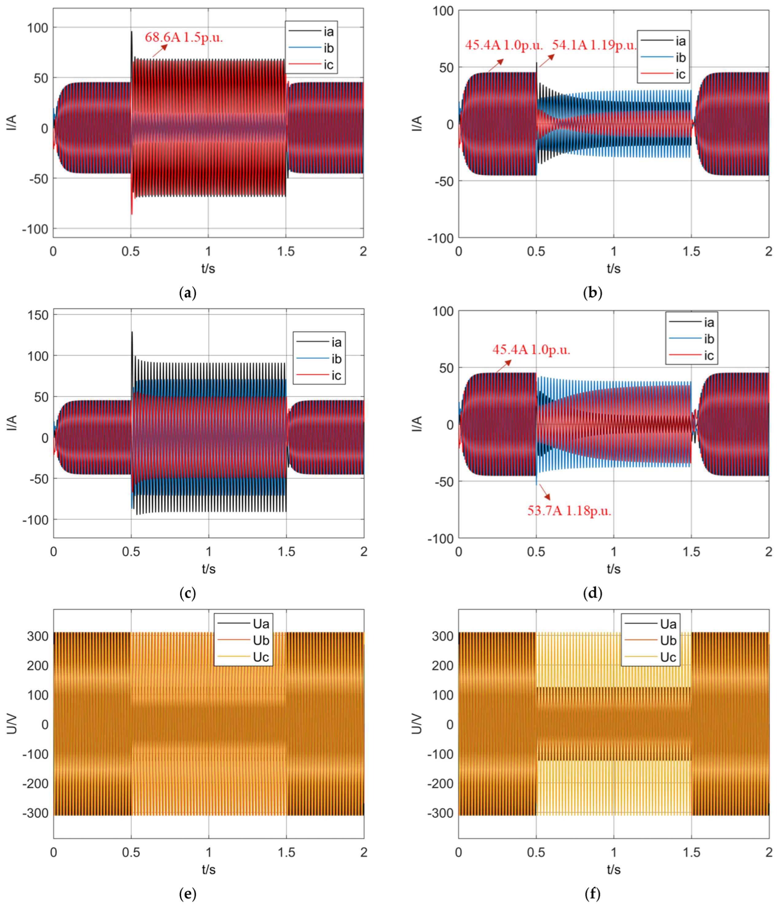
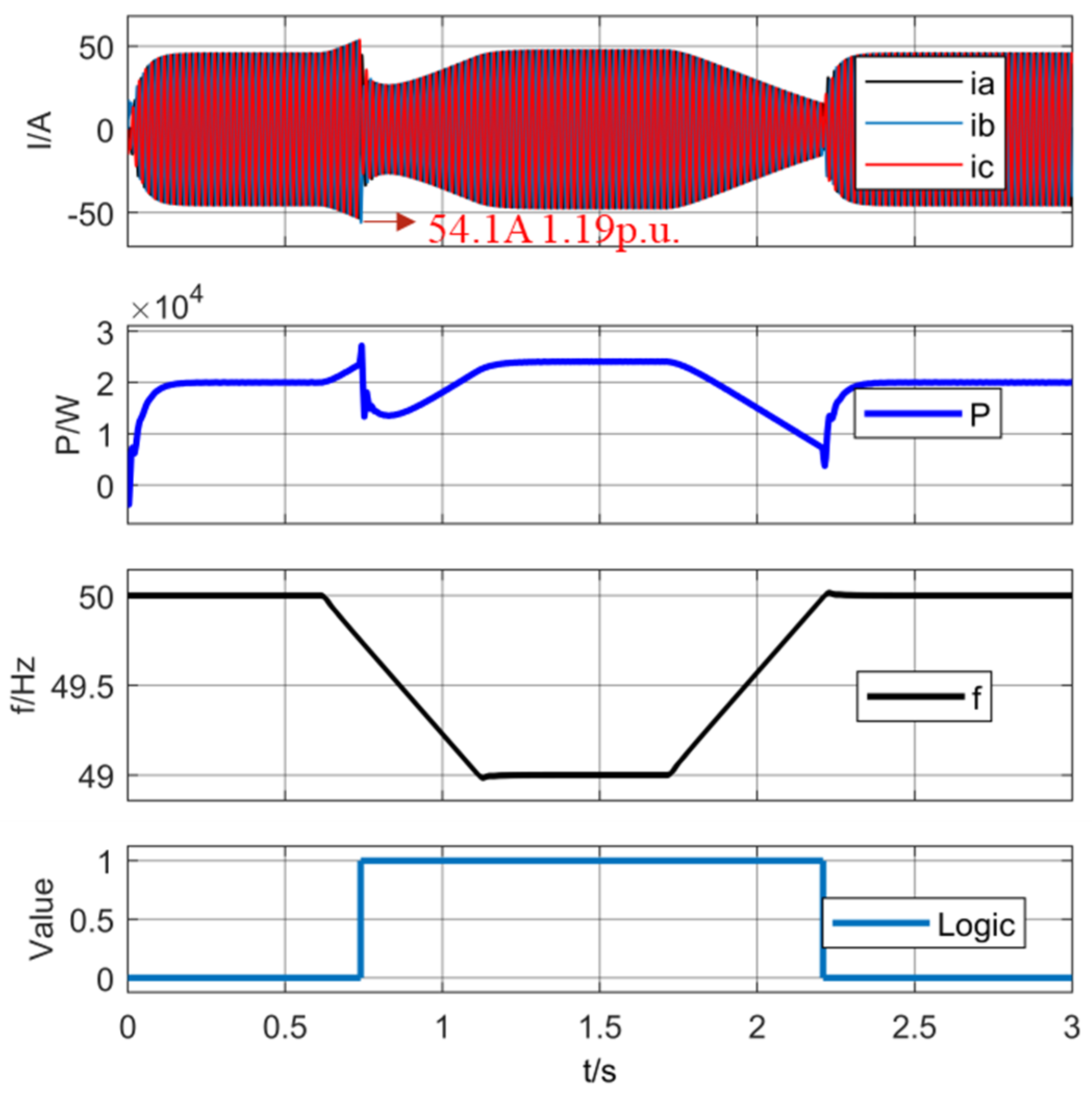
5.1. Simulation Verification

The proposed switching logic of the virtual impedance and the dynamic current limitation scheme are verified by the simulation tests. The voltage drops of 40% and 60% occurred at 0.5 s and returned subsequently to normal conditions at 1.5 s. The main parameters of the simulation tests are listed in

Table 3. Main simulation parameters.

Parameter	Value	Parameter	Value
DC bus voltage Udc	800 V	Grid-side equivalent inductance Lg	5 mH
Switching frequency fs	10 kHz	Grid-side equivalent resistance Rg	0.9 Ω
Inductance Lf	10 mH	Reactive droop coefficient Dq	3 × 10−4
Capacitance Cf	50 μF	Active droop coefficient Dp	3.33 × 10−4
Current controller P gain kip	50	Active power reference Pref	20 kW
Virtual resistor Rv	1 Ω	Voltage controller P gain kup	0.5
Virtual inductance Lv	5 mH	Voltage controller I gain kui	100
Voltage magnitude reference value E	311 V	Frequency reference ωref	50 Hz

. The simulation model is based on MatLab/Simulink R2022a. In addition, the control logic triggers the interruption on time, and the protection logic triggers the interruption on event.

Figure 10a shows the output current of the GFM inverter without the dynamic current limitation with a 40% voltage drop. The instantaneous peak current is 1.92 p.u., and the current at stability is 1.52 p.u. during the grid fault. In contrast, Figure 10b depicts the output current of the GFM inverter with dynamic current limitation. The peak current is 1.18 p.u., and overcurrent can be avoided, which verified the effectiveness of the proposed method. Additionally, Figure 10b,d indicate that after the fault clearance, the output current of the GFM inverter recovers to its normal value. From Figure 10e, it can be seen that when overcurrent is detected in the system, the logic for enabling virtual impedance remains at a high level. After fault clearance, the logic for enabling virtual impedance is switched to a low level, and virtual impedance is effectively enabled and disabled during grid fault and fault clearance. From Figure 10g,h, it can be seen that overcurrent occurs only at the moment of grid-voltage drop, which indicates that the virtual impedance activation limits the current.

Figure 10c illustrates the output current of the GFM inverter without dynamic current limitation in the case of a grid-voltage drop of 60%. It can be seen that the GFM inverter becomes unstable. It is obvious that the fault current exceeds 2 p.u., which is much higher than the current threshold. Conversely, Figure 10d shows the simulation result of the dynamic current limitation strategy: the GFM inverter remains stable under grid fault with an instantaneous maximum current of 1.22 p.u., which is lower than the current limitation. Moreover, from Figure 10f, it can be observed that the reference of the active power is set to zero for maximizing the reactive power injection without overcurrent. After fault clearance, the active power quickly returns to the desired value. It can be seen from Figure 10i,j that when the grid-voltage drops by 60%, the injected reactive power plays a certain role in voltage support.

It can be seen from the comparison between Figure 10b and Figure 10k and Figure 10d and Figure 10l that the impact current of the event-triggered current limitation strategy is significantly lower than that of the traditional time-triggered strategy. This shows that the event triggering based on the SR latch accelerates the speed of current control, and the switching strategy can be implemented immediately after the voltage drops and the current increases to achieve current suppression. In addition, it can be found that the transient current is smaller because of the event-triggering function of the SR latch.

Since the probability of three-phase voltage drop is low, this paper simulated single-phase voltage drop and two-phase voltage drop, respectively, and the simulation results are shown in Figure 11.

Figure 11a shows the output current of the GFM inverter without dynamic current limitation with a 60% A-phase voltage drop. The steady-state value of the output current is 1.5 p.u., which exceeds the current. In contrast, Figure 11b depicts the output current of the GFM inverter with dynamic current limitation. The peak current is 1.19 p.u., and overcurrent can be avoided, which verifies the effectiveness of the proposed method. Additionally, Figure 11c,d are the output current diagram of the two-phase voltage drop. Among them, since Figure 11c does not add dynamic current limiting, it exceeds the current limitation during the two-phase voltage drop. On the contrary, the peak output current with dynamic current limitation is only 1.18 p.u., which shows that it does not exceed the current limitation. Although the output current during the fault is asymmetrical, the device integrity during the fault is guaranteed.

In order to further demonstrate the effectiveness and applicability of the proposed method, the droop control with a low-pass filter with a time constant equivalent of 5 s is validated in this paper. The grid frequency drops to 49 Hz at 0.6 s, and rises to 50 Hz at 1.7 s, with a slope of 2 Hz/s.

As can be seen from Figure 12, when the power grid frequency drops at a rate of 2 Hz/s, the output current of the inverter begins to gradually increase. When the current increases to the threshold, the protection logic of the SR latch is triggered, and then changes in the amount of active and reactive power are compared to select the maximum support of the active or reactive power, and finally the virtual impedance is enabled. In addition, the active power also decreases due to virtual impedance, but the active power recovers quickly, and thus active power support is provided for the grid. The output current is also within a feasible range, and there is no overcurrent phenomenon. When the grid frequency recovers, the virtual impedance is disabled and grid-forming control operates normally.

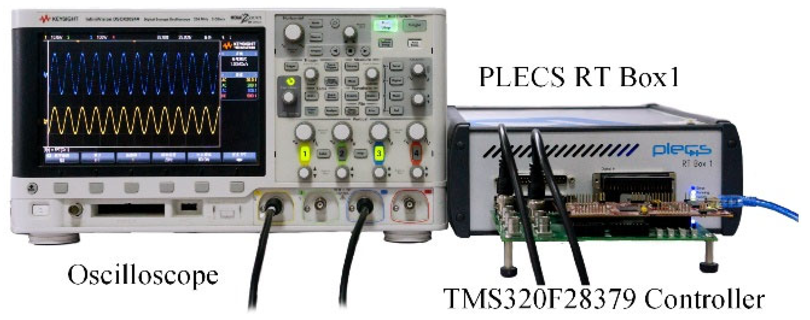
5.2. Experiment Verification

To solve practical sensing issues and further verify the accuracy of the proposed dynamic current-limitation strategy based on SR latches, tests are conducted on a HIL experiment platform based on the RT-Box from PLECS as shown in Figure 13. On the platform, a TMS320F28379D from Texas Instruments is used as the digital controller and the three-phase droop-controlled inverter is simulated on the RT-Box. The main parameters of the experiment tests are listed in

Table 4. Main experiment parameters.

Parameter	Value	Parameter	Value
DC bus voltage Udc	800 V	Grid-side equivalent inductance Lg	10 mH
Switching frequency fs	10 kHz	Current controller I gain kii	333
Inductance Lf	3 mH	Reactive droop coefficient Dq	2 × 10−4
Capacitance Cf	100 μF	Active droop coefficient Dp	3 × 10−4
Current controller P gain kip	30	Active power reference Pref	20 kW
Virtual resistor Rv	2 Ω	Voltage controller P gain kup	0.15
Virtual inductance Lv	5 mH	Voltage controller I gain kui	75
Voltage magnitude reference value E	311 V	Frequency reference ωref	50 Hz

.

Figure 14a shows the experimental output current of the GFM inverter and logic value without dynamic current limitation with a 40% voltage drop. Compared with Figure 14b, it can be found that after detecting an overcurrent signal, the virtual impedance is immediately enabled, and there is no sensing-delay issue. In addition, it can also be seen that the proposed dynamic current-limitation strategy can suppress an overcurrent well.

Further, it can be seen from Figure 14c,d that the output current without considering the dynamic current-limitation strategy has become unstable, and even the grid-voltage recovery fails to restore the steady state. However, the inverter with dynamic current limitation can limit the overcurrent problem well, and the activation and deactivation of virtual impedance can also be well adapted to it, indicating that the sensing problem can be ignored.

6. Conclusions

In this paper, the grid-forming control scheme is first introduced for a three-phase inverter, and the fault current dynamic is analyzed under different grid faults. Then, the fault current limitation method is proposed for the GFM inverter under grid drop. The simulation and experimental results verify the effectiveness of the proposed method. The following conclusions can be drawn:

• SR latch-based virtual impedance control scheme can retain current-limitation ability during grid fault. In addition, compared with other current-limitation schemes, the proposed current-limitation method can not only avoid the saturation of the voltage loop, but also avoid the repeated switching of virtual impedance.
• Virtual impedance control with a power modification can effectively achieve fault current limitation without synchronization instability problems during grid fault.
• The event-triggered control logic is applied in a digital controller, which can suppress the inrush current induced by time delay.

References

1. Han, X.; LI, T.; Zhang, D. New Issues and Key Technologies of New Power System Planning under Double Carbon Goals. High Volt. Eng. 2021, 346, 3036–3046. [Google Scholar]
2. Liu, Y.; Chen, L.; Han, X. The Key Problem Analysis on the Alternative New Energy under the Energy Transition. Proc. CSEE 2022, 42, 515–524. [Google Scholar]
3. Xu, J.; Liu, W.; Liu, S. Current State and Development Trends of Power System Converter Grid-forming Control Technology. Power Syst. Technol. 2022, 46, 3586–3595. [Google Scholar]
4. Zhou, X.; Chen, S.; Lu, Z. Technology Features of the New Generation Power System in China. Proc. CSEE 2018, 38, 1893–1904+2205. [Google Scholar]
5. Taul, M.G.; Wang, X.; Davari, P. An Overview of Assessment Methods for Synchronization Stability of Grid-Connected Converters under Severe Symmetrical Grid Faults. IEEE Trans. Power Electron. 2019, 34, 9655–9670. [Google Scholar] [CrossRef]
6. Ebinyu, E.; Abdel-Rahim, O.; Mansour, D.A.; Shoyama, M.; Abdelkader, S.M. Grid-Forming Control: Advancements towards 100% Inverter-Based Grids—A Review. Energies 2023, 16, 7579. [Google Scholar] [CrossRef]
7. Zhang, H.; Xiang, W.; Lin, W.; Wen, J. Grid Forming Converters in Renewable Energy Sources Dominated Power Grid: Control Strategy, Stability, Application, and Challenges. J. Mod. Power Syst. Clean Energy 2021, 9, 1239–1256. [Google Scholar] [CrossRef]
8. Henninger, S.; Schroeder, M.; Jaeger, J. Grid-Forming Droop Control of a Modular Multilevel Converter in Laboratory. In Proceedings of the 2018 IEEE Power & Energy Society General Meeting (PESGM), Portland, OR, USA, 5–10 August 2018. [Google Scholar]
9. D’Arco, S.; Suul, J.A. Equivalence of Virtual Synchronous Machines and Frequency-Droops for Converter-Based MicroGrids. IEEE Trans. Smart Grid 2014, 5, 394–395. [Google Scholar] [CrossRef]
10. Liu, J.; Miura, Y.; Ise, T. Comparison of Dynamic Characteristics Between Virtual Synchronous Generator and Droop Control in Inverter-Based Distributed Generators. IEEE Trans. Power Electron. 2015, 31, 3600–3611. [Google Scholar] [CrossRef]
11. Ding, M.; Yang, X.; Su, X. Microgrid inverter power supply control strategy based on the idea of virtual synchronous generator. Autom. Electr. Power Syst. 2009, 33, 89–93. [Google Scholar]
12. Sakimoto, K.; Miura, Y.; Ise, T. Stabilization of a power system with a distributed generator by a Virtual Synchronous Generator function. In Proceedings of the 8th International Conference on Power Electronics—ECCE Asia, Jeju, Republic of Korea, 30 May–3 June 2011; pp. 1498–1505. [Google Scholar]
13. Baltas, G.N.; Lai, N.B.; Marini, L. Grid-forming Power Converter controller with Artificial Intelligence to Attenuate Inter-Area Modes. In Proceedings of the 2020 IEEE 21st Workshop on Control and Modeling for Power Electronics (COMPEL), Aalborg, Denmark, 9–12 November 2020; IEEE: Piscataway, NJ, USA, 2020. [Google Scholar]
14. Seo, G.S.; Colombino, M.; Subotic, I. Dispatchable Virtual Oscillator Control for Decentralized Inverter-dominated Power Systems: Analysis and Experiments. In Proceedings of the Applied Power Electronics Conference, Anaheim, CA, USA, 17–21 March 2019; IEEE: Piscataway, NJ, USA, 2019. [Google Scholar]
15. Zhao, X.; Flynn, D. Freezing Grid-Forming Converter Virtual Angular Speed to Enhance Transient Stability under Current Reference Limiting. In Proceedings of the 2020 IEEE 21st Workshop on Control and Modeling for Power Electronics (COMPEL), Aalborg, Denmark, 9–12 November 2020; IEEE: Piscataway, NJ, USA, 2020. [Google Scholar]
16. Li, T.; Li, Y.; Chen, X.; Li, S.; Zhang, W. Research on AC Microgrid with Current-Limiting Ability Using Power-State Equation and Improved Lyapunov-Function Method. IEEE J. Emerg. Sel. Top. Power Electron. 2021, 9, 7306–7319. [Google Scholar] [CrossRef]
17. Mahamedi, B.; Eskandari, M.; Fletcher, J.E.; Zhu, J. Sequence-Based Control Strategy with Current Limiting for the Fault Ride-Through of Inverter-Interfaced Distributed Generators. IEEE Trans. Sustain. Energy 2020, 11, 165–174. [Google Scholar] [CrossRef]
18. Fan, B.; Wang, X. Fault Recovery Analysis of Grid-Forming Inverters with Priority-Based Current Limiters. IEEE Trans. Power Syst. 2023, 38, 5102–5112. [Google Scholar] [CrossRef]
19. Camacho, A.; Castilla, M.; Miret, J. Active and Reactive Power Strategies with Peak Current Limitation for Distributed Generation Inverters During Unbalanced Grid Faults. IEEE Trans. Ind. Electron. 2015, 62, 1515–1525. [Google Scholar] [CrossRef]
20. Paquette, A.; Divan, D. Virtual Impedance Current Limiting for Inverters in Microgrids with Synchronous Generators. IEEE Trans. Ind. Appl. 2015, 51, 1630–1638. [Google Scholar] [CrossRef]
21. Lu, X.; Wang, J.; Guerrero, J.M.; Zhao, D. Virtual-Impedance-Based Fault Current Limiters for Inverter Dominated AC Microgrids. IEEE Trans. Smart Grid 2018, 9, 1599–1612. [Google Scholar] [CrossRef]
22. Wu, H.; Wang, X. Small-Signal Modeling and Controller Parameters Tuning of Grid-Forming VSCs with Adaptive Virtual Impedance-Based Current Limitation. IEEE Trans. Power Electron. 2022, 37, 7185–7199. [Google Scholar] [CrossRef]
23. Xiong, X.; Wu, C.; Blaabjerg, F. Effects of Virtual Resistance on Transient Stability of Virtual Synchronous Generators under Grid Voltage Sag. IEEE Trans. Ind. Electron. 2022, 69, 4754–4764. [Google Scholar] [CrossRef]
24. Wang, P.; Wang, P.; Li, S. Dynamic Current-Limiting Control Strategy of Grid-Forming Inverter under Grid Fault. High Volt. Eng. 2022, 48, 3829–3837. [Google Scholar]
25. Shang, L.; Hu, J.; Yuan, X. Modeling and Improved Control of Virtual Synchronous Generators under Symmetrical Faults of Grid. Proc. CSEE 2017, 37, 403–412. [Google Scholar]
26. Zhou, L.; Liu, S.; Chen, Y.; Yi, W.; Wang, S.; Zhou, X.; Wu, W.; Zhou, J.; Xiao, C.; Liu, A. Harmonic Current and Inrush Fault Current Coordinated Suppression Method for VSG under Non-ideal Grid Condition. IEEE Trans. Power Electron. 2021, 36, 1030–1042. [Google Scholar] [CrossRef]
27. Erdocia, J.; Urtasun, A.; Marroyo, L. Dual Voltage–Current Control to Provide Grid-Forming Inverters with Current Limiting Capability. IEEE J. Emerg. Sel. Top. Power Electron. 2022, 10, 3950–3962. [Google Scholar] [CrossRef]
28. Fan, B.; Wang, X. Equivalent Circuit Model of Grid-Forming Converters with Circular Current Limiter for Transient Stability Analysis. IEEE Trans. Power Syst. 2022, 37, 3141–3144. [Google Scholar] [CrossRef]
29. Huang, L.; Xin, H.; Wang, Z.; Zhang, L.; Wu, K.; Hu, J. Transient Stability Analysis and Control Design of Droop-Controlled Voltage Source Converters Considering Current Limitation. IEEE Trans. Smart Grid 2019, 10, 578–591. [Google Scholar] [CrossRef]
30. Zhuang, K.; Xin, H.; Hu, P.; Wang, Z. Current Saturation Analysis and Anti-Windup Control Design of Grid-Forming Voltage Source Converter. IEEE Trans. Energy Convers. 2022, 37, 2790–2802. [Google Scholar] [CrossRef]
31. Laaksonen, H.; Saari, P.; Komulainen, R. Voltage and frequency control of inverter based weak LV network microgrid. In Proceedings of the 2005 International Conference on Future Power Systems, Amsterdam, The Netherlands, 18 November 2005; IEEE: Piscataway, NJ, USA, 2005. [Google Scholar]
32. Xu, F.; Hu, C.; Wang, F. Research on Droop Control Strategy of Improved Gird-connected Inverters. High Volt. Appar. 2017, 53, 106–112. [Google Scholar]
33. Li, Y.; Gu, Y.; Zhu, Y. Impedance Circuit Model of Grid-Forming Inverter: Visualizing Control Algorithms as Circuit Elements. IEEE Trans. Power Electron. 2021, 36, 3377–3395. [Google Scholar] [CrossRef]
Figure 1. GFM inverter schematic diagram.
Electronics 13 03432 g001
Figure 2. Switching logic of virtual impedance.
Electronics 13 03432 g002
Figure 3. Grid-forming inverter control system.
Electronics 13 03432 g003
Figure 4. Simplified model diagram of GFM inverters.
Electronics 13 03432 g004
Figure 5. Block diagram of the droop control with a low-pass filter.
Electronics 13 03432 g005
Figure 6. Equivalent circuit model of GFM inverters during grid faults.
Electronics 13 03432 g006
Figure 7. Block diagram of voltage-current dual-loop control with virtual impedance.
Electronics 13 03432 g007
Figure 8. Power limitation-control block diagram for GFM inverters.
Electronics 13 03432 g008
Figure 9. Dynamic current-limitation implementation flow chart.
Electronics 13 03432 g009
Figure 10. Low-voltage ride-through waveforms for GFM inverters. (a) The output current of the GFM inverter without dynamic current limitation after a 40% grid-voltage drop; (b) the output current of the GFM inverter with dynamic current limitation after a 40% grid-voltage drop; (c) the output current of the GFM inverter without dynamic current limitation after a 60% grid-voltage drop; (d) the output current of the GFM inverter with dynamic current limitation after a 60% grid-voltage drop. (e) Logic for virtual impedance activation and deactivation; (f) active power output of GFM inverter with dynamic current limitation; (g) Logic for grid-voltage recovery; (h) logic for overcurrent detection. (i) The output voltage of the GFM inverter with dynamic current limitation after a 60% grid-voltage drop; (j) the output reactive power of the GFM inverter with dynamic current limitation after a 60% grid-voltage drop. (k) The time triggers of the output current waveform after a 40% grid-voltage drop; (l) The time triggers of the output current waveform after a 60% grid-voltage drop.
Electronics 13 03432 g010aElectronics 13 03432 g010b
Figure 11. Low-voltage ride-through waveforms for GFM inverters under asymmetric failure. (a) The output current of the GFM inverter without dynamic current limitation after a 60% A-phase grid-voltage drop; (b) the output current of the GFM inverter with dynamic current limitation after a 60% A-phase grid-voltage drop; (c) the output current of the GFM inverter without dynamic current limitation after a 60% AB-phases grid-voltage drop; (d) the output current of the GFM inverter with dynamic current limitation after a 60% AB-phases grid-voltage drop; (e) A-phase grid-voltage drop waveform; (f) AB-phases grid-voltage drop waveform.
Electronics 13 03432 g011
Figure 12. Grid-frequency drop waveform.
Electronics 13 03432 g012
Figure 13. Experimental platform.
Electronics 13 03432 g013
Figure 14. Low-voltage ride-through experimental waveforms for GFM inverter. (a) The output current of the GFM inverter and logic value without dynamic current limitation after a 40% grid-voltage drop; (b) the output current of the GFM inverter and logic value with dynamic current limitation after a 40% grid-voltage drop; (c) the output current of the GFM inverter and logic value without dynamic current limitation after a 60% grid-voltage drop; (d) the output current of the GFM inverter and logic value with dynamic current limitation after a 60% grid-voltage drop.
Electronics 13 03432 g014