Research on Control Strategy of Oscillating Continuous-Wave Pulse Generator Based on ILADRC

Abstract

To achieve fast and precise position servo control in a continuous-wave pulse generator and address issues such as internal and external disturbances and significant overshoot, this paper proposes an improved linear active disturbance rejection control strategy. First, a mathematical model of the permanent magnet synchronous motor is established, and a second-order linear active disturbance rejection controller is designed based on this model. To address the issue of large errors in disturbance estimation by the traditional extended state observer, a cascaded extended state observer is introduced. By designing an additional state observer to estimate the system’s residual disturbances, the impact of disturbances on system performance is further reduced. Through an in-depth analysis of the motion characteristics of the continuous-wave pulse generator, the trade-off between system overshoot and response speed is revealed. To address this, a new adaptive law is proposed. This law, based on the system’s periodic wave response and tracking error, adjusts the parameters of the linear state error feedback control law in real time, reducing system overshoot while improving response speed. To validate the effectiveness of the proposed control strategy, a simulation model of the position servo control system for the continuous-wave pulse generator was developed. The comparative analysis of the simulation results for the different control strategies shows that the improved linear active disturbance rejection control strategy significantly enhances the system’s dynamic response performance.

1. Introduction

Measurement While Drilling (MWD) technology can measure and obtain engineering parameters such as inclination, azimuth, and tool face in real time during drilling [1,2]. It is the key core technology of oil and gas exploration and development. The continuous-wave pulse generator is widely used in MWD information transmission due to its high stability and reliability, as well as the advantages of the high-speed long-distance transmission of mud pressure signal generated by it [3]. Permanent magnet synchronous motor (PMSM) is a driving component of the continuous-wave pulse generator, and its control results directly determine the quality of the mud pressure signal and the transmission rate of MWD [4]. To improve the control performance of PMSM, advanced control strategies such as sliding mode control (SMC) [5,6], fuzzy control [7], and model predictive control (MPC) [8,9] have been proposed, but these strategies have excellent control performance and some limitations. For example, SMC will inevitably produce high-frequency oscillation near the sliding mode surface [10]. The membership functions and fuzzy rules of fuzzy control rely too much on expert experience and intuitive judgment [11]. It is difficult to solve the problem that MPC requires a large amount of computation and high model accuracy [12].

In the 1990s, Professor Han Jingqing proposed active disturbance rejection control (ADRC). The basic idea of ADRC is to obtain disturbance information autonomously and eliminate it with control signals before the disturbance significantly affects the final output of the system, thus greatly reducing the influence of the disturbance on the controlled quantity [13]. ADRC has been extensively studied for its excellent anti-disturbance performance. In the literature [14], an adaptive extended state observer was used to estimate the state and total disturbance of electric heating furnace systems, in which the observer gains are updated online by a nonlinear observer bandwidth, and simulation results show that the proposed method has excellent robustness and temperature tracking performance. The literature [15] deduced the necessary conditions for ADRC to ensure the stability of the closed-loop system, and theoretically analyzed the advantages of ADRC in sensor noise suppression and control signal change. The literature [16] constructs a new nonlinear function by using inverse hyperbolic sine function, quadratic function, and tangential function. The reconstructed optimal control function can effectively improve the smoothness of the nonlinear function and ensure that it is differentiable at the piecewise position, which effectively improves the robustness of ADRC. However, the nonlinear function parameters adopted by ADRC are large and complicated to adjust, so it is difficult to achieve simple and fast control in practical applications [17,18]. After more than ten years of development, ADRC finally realized linear active disturbance rejection control (LADRC). LADRC consists of linear extended state observer (LESO) and linear state error feedback (LSEF). Compared with ADRC, LADRC is not only more intuitive in the physical sense, but also greatly reduces the number of parameters to be adjusted to three [19,20], so it is widely used in practical engineering control.

The core of LADRC is to eliminate LESO’s estimation of unknown disturbances from the system. Therefore, LESO is the key to LADRC. The current research on LESO can be divided into two aspects: improving its anti-interference ability and improving its disturbance-tracking characteristics. Aiming at the anti-interference capability of LADRC, the literature [21] explained LESO from the perspective of a filter, indicating that the core of LESO is a low-pass filter, and proposed a parameter tuning method for LESO. Reference [22] introduces fractional calculus to improve the noise robustness of the system without affecting the control performance. In the literature [23], a variable gain LESO was designed to compensate for the disturbance, and combined with the Kalman filter, the noise can be measured and suppressed in real time. The experimental results show that the proposed control strategy can improve the noise robustness of the servo system. However, the disturbance-tracking capability of this strategy still needs to be improved. Therefore, a compensator based on adaptive switching function is introduced in the literature [24] to eliminate the observation error and reduce the adjustment range of the observer bandwidth. The literature [25] enhanced the estimation ability of the system to the disturbance by adding the error proportional feedback term to the extended state observer. The literature [26] proposed a fractal-order LESO, adding fractal-order terms to the framework of traditional LESO to reduce disturbance estimation errors and make the design of LESO more flexible.

In addition, the research on LADRC is not limited to LESO. For example, the literature [27] shows that LADRC is a universal control structure, and the internal relationship between different linear controllers is revealed through the LADRC structure. The literature [28] improved LADRC by replacing the traditional cascade structure of PMSM position and velocity loops with a novel parallel structure, which improved the dynamic response and anti-disturbance performance of the system. In the literature [29], combining the U-type control and Glover–McFarlane control ideas, the proposed robust U-type active interference suppression controller replaces the traditional LADRC PD controller, which reduces the lag time of extreme points between input and output. At the same time, to overcome the degradation of LADRC performance caused by the change in system state or external environment, much research has achieved rich results. For example, the literature [30] proposes an adaptive law to adjust the scale coefficient and differential coefficient of LADRC, and adjusts a large number of adjustable parameters in the controller through the improved particle swarm optimization algorithm. In the literature [31], the differential evolution algorithm was designed to find optimal controller parameters with self-tuning to solve the problem of system parameter changes. The literature [32] proposes an adaptive law for LADRC and the time-varying coefficient of the high-speed train system, effectively eliminating the adverse effects of the time-varying coefficient on train operation.

The above research has promoted the development of the LADRC theory and achieved remarkable results. In the relevant research, improving LESO’s estimation ability of complex perturbations is always the focus of LADRC research. However, there are still relatively few research on how to use the system’s own information to improve the control performance for specific controlled objects.

In view of the above challenges, the improved linear active disturbance rejection control (ILADRC) is proposed in this paper to improve the control performance of the oscillating continuous-wave pulse generator. By introducing cascade linear expanded state observer (CLESO), this method reduces the estimation error of the observer to the disturbance and improves the anti-interference ability of the system. Then, an adaptive law based on periodic wave response and tracking error is proposed to adjust the proportion and differential coefficient of LSEF in real time, which reduces the overshoot and improves the response speed of the system.

The rest of this paper is organized as follows: The second section explains the working principle of the continuous-wave pulse generator and the mathematical model of PMSM, builds the traditional LADRC based on the mathematical model, and analyzes the shortcomings of LESO. In the third section, the ILADRC strategy is introduced, the CLESO model is established, and the observer disturbance estimate, and the actual disturbance transfer function are obtained. In addition, the overshot problem of the oscillating continuous-wave pulse generator is analyzed, and a new adaptive law is proposed. In the fourth section, the performance of different control strategies is compared and analyzed by setting up the simulation model of position servo control of a continuous-wave pulse generator. Finally, see section five for conclusions.

2. Mathematical Model

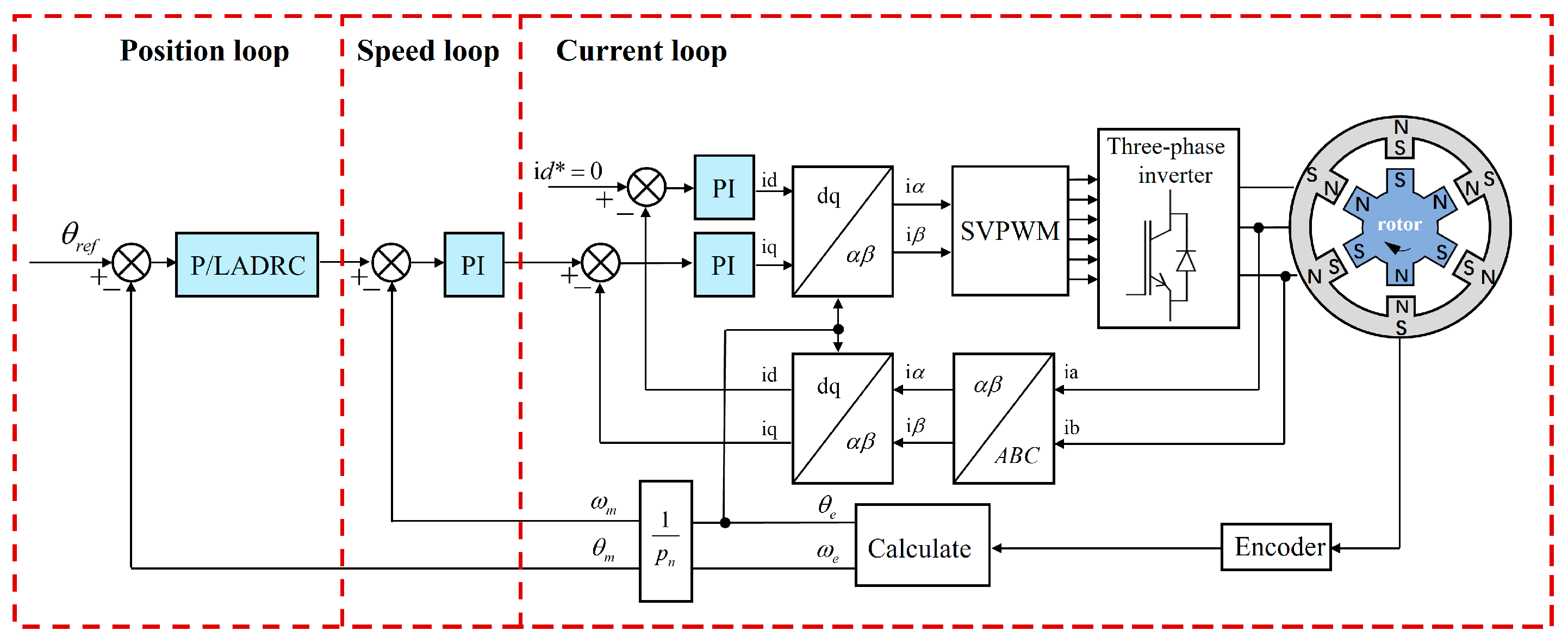
2.1. Oscillating Continuous-Wave Pulse Generator Working Principle

The oscillating continuous-wave pulse generator is an important part of the high-speed mud pulse remote transmission system while drilling [33], which is used to generate mud pressure wave signals, and its main components include PMSM, reducer, shear valve, drive control circuit, etc., as shown in Figure 1.

The shear valve is the key component of pressure signal generation. It consists of a stator and rotor; the stator and rotor are designed to have a special shape. As the rotor rotates, the mud pressure at the valve port shows a sinusoidal waveform. PMSM drives the shear valve rotor to swing back and forth, and then changes the throttle area so that the mud pressure is constantly changing. To make the mud pressure signal carry information and ensure the robustness of data transmission, the pressure signal must be modulated. The Quadrature Phase Shift Keying (QPSK) modulation method is used in this paper [34,35]. QPSK specifies four carrier phases, whose waveforms are shown in Figure 2. Each phase represents a set of binary double-bit code elements, namely “00”, “01”, “10” and “11”. By controlling PMSM, the shear valve rotor can track the angular input waveform of QPSK and accurately change the mud throttling area of the pulse generator so that the mud pressure in the channel generates waveform signals specified by QPSK, and the pressure waves are transmitted to the surface through the drill string, and the downhole information can be obtained after being collected and decoded by the surface signal-processing equipment.

According to the simplified thin-wall pressure drop calculation model [36], the relationship between the pressure drop generated by the shear valve and the throttling area of the shear valve can be expressed as Equation (1).

$$\Delta p_t={\displaystyle \frac{\rho }{2{K_d}^2}}{({\displaystyle \frac{Q_t}{S_t}})}^2$$

(1)

where $\Delta p_t$ is the pressure drop generated by the shear valve; $S_t$ is the throttle area of the shear valve; $Q_t$ is the mud flow rate; $K_d$ is the flow coefficient of the shear valve port; and $\rho$ is the mud density.

It can be seen from Equation (1) that when the mud flow rate is fixed, the pressure drop generated by the shear valve is inversely proportional to the square of its throttling area; that is, the larger the throttling area, the smaller the pressure drop and the smaller the pressure amplitude. Therefore, precisely controlling the PMSM to change the throttle area of the shear valve is a prerequisite for the continuous-wave pulse generator to generate QPSK pressure waves.

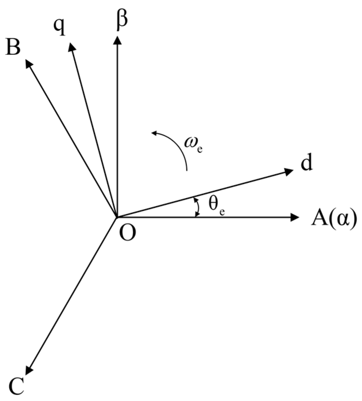
2.2. Mathematical Model of PMSM

To simplify the mathematical model of three-phase PMSM in a natural coordinate system, coordinate transformation usually includes stationary coordinate transformation (Clark transformation) and synchronous rotation coordinate transformation (Park transformation). The coordinate relationship between them is shown in Figure 3, where ABC is the natural coordinate system, $\alpha -\beta$ is the stationary coordinate system, and $d-q$ is the synchronous rotating coordinate system.

To realize the control of PMSM, the mathematical model of PMSM is established in the synchronous rotating coordinate system [37,38].

The voltage equation is shown below.

$$\left\{\begin{array}{l}{u}_d=R{i}_d+L_d{\displaystyle \frac{d}{dt}}{i}_d-{\omega }_e{L}_q{i}_q\hfill \\ u_q=R{i}_q+L_q{\displaystyle \frac{d}{dt}}{i}_q+{\omega }_e(L_d{i}_d+{\phi }_f)\hfill \end{array}\right.$$

(2)

where $L_d$, $L_q$, $i_d$, $i_q$, $u_d$, and $u_q$, respectively, represents the components of stator inductance, current, and voltage on the axes $d-q$; ${\omega }_e$ is the electric angular velocity; and ${\phi }_f$ is the permanent magnet flux linkage.

The electromagnetic torque equation is shown below.

$$T_e={\displaystyle \frac{3}{2}}{p}_n{i}_q[i_d(L_d-L_q)+{\phi }_f]$$

(3)

where $T_e$ is electromagnetic torque; $p_n$ is the number of magnetic poles of the motor.

PMSM can be divided into surface mount type ($L_d=L_q$) and built-in type ($L_d\ne L_q$) according to the different installation positions of the permanent magnets on the rotor core. In this paper, the continuous-wave pulse generator is driven by a surface-mount PMSM. At the same time, to ensure the complete synchronization of the stator magnetic field and the rotor magnetic field, and to accurately control the motor speed and torque, $i_d=0$ is generally controlled by the magnetic field orientation [39]. Therefore, Equation (2) can be simplified as Equation (4).

$$\left\{\begin{array}{l}{u}_d=-{\omega }_e{L}_q{i}_q\hfill \\ u_q=R{i}_q+L_q{\displaystyle \frac{d}{dt}}{i}_q+{\omega }_e{\phi }_f\hfill \end{array}\right.$$

(4)

The electromagnetic torque equation is reduced to Equation (5).

$$T_e={\displaystyle \frac{3}{2}}{p}_n{i}_q{\phi }_f$$

(5)

It can be seen from Equation (5) that controlling $q$ axis current $i_q$ can directly control electromagnetic torque $T_e$. In addition, to realize the Angle control of continuous wave pulser PMSM, the motion equation is constructed as follows:

$$J{\ddot{\theta }}_m=T_e-T_L-B{\omega }_{\mathrm{m}}$$

(6)

where $J$ is the moment of inertia of the mechanical part; ${\theta }_m$ is PMSM mechanical angular velocity; $T_L$ is the load torque; and $B$ is the damping coefficient.

The load torque of the oscillating continuous-wave pulse generator PMSM is mainly the hydraulic torque received by the shear valve rotor, which can be expressed as Equation (7).

$$\left\{\begin{array}{l}M=M_s+M_t\hfill \\ M_s=\rho \xi \left(Q_s{v}_s\cos {\theta }_s-Q_{sr}{v}_{sr}\right)r\hfill \\ M_t=-\dot{\omega }{J}_w\hfill \end{array}\right.$$

(7)

where $M_s$ is the steady-state hydraulic torque; $M_t$ is the transient hydraulic torque; $\xi$ is the diffusion coefficient, $\xi$ increases with the increase in rotor blade wall thickness; and $Q_s$, $v_s$, and ${\theta }_s$ are, respectively, the flow rate, velocity, and jet Angle of the slurry at the stator of the shear valve. $Q_{sr}$ and $v_{sr}$ are the leakage of mud flow and velocity at the gap between the stator and the rotor of the shear valve; $r$ is the radius of the middle surface of the flow in the rotor area; $\omega$ is the angular speed of the shear valve rotor; and $J_r$ is the moment of inertia of the fluid in the rotor region with respect to the rotating shaft.

Since the transient hydraulic torque of an oscillating continuous-wave pulse generator is much smaller than the steady-state hydraulic torque, it is generally ignored [40]. In addition, it can be seen from Equation (7) that the steady-state hydraulic torque is related to the rotor Angle of the shear valve. The research shows that the hydraulic torque of continuous-wave pulse generator PMSM in the borehole is like that of a sine wave. When the shear valve is gradually closed, the hydraulic torque keeps increasing, and the hydraulic torque is maximum when the shear valve is completely closed. When the shear valve is gradually opened, the hydraulic torque keeps decreasing, and the hydraulic torque is minimum when it is completely opened. Its frequency and phase are close to the motion law of the shear valve rotor [41,42].

By combining Equations (5)–(7), the relationship between the current and Angle of the continuous-wave pulse generator PMSM is finally obtained as shown below.

$$J{\ddot{\theta }}_m={\displaystyle \frac{3}{2}}{p}_n{i}_q{\phi }_f-\rho \xi \left(Q_s{v}_s\cos {\theta }_s-Q_{sr}{v}_{sr}\right)r-B{\omega }_{\mathrm{m}}$$

(8)

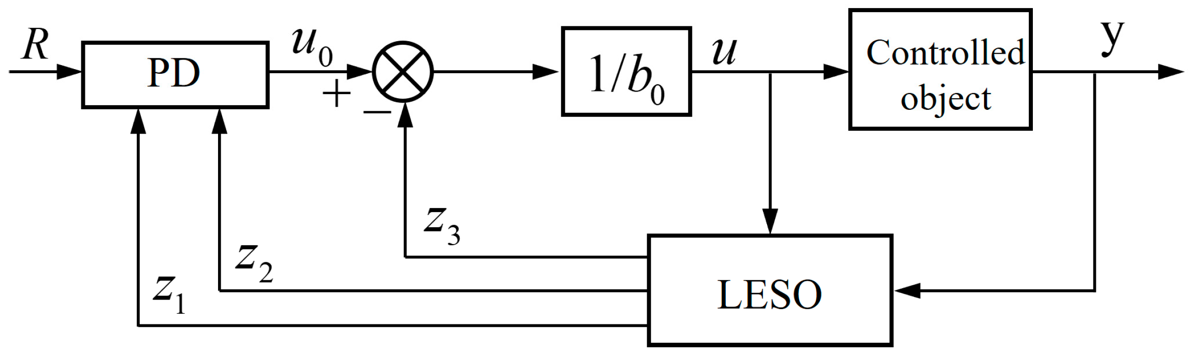
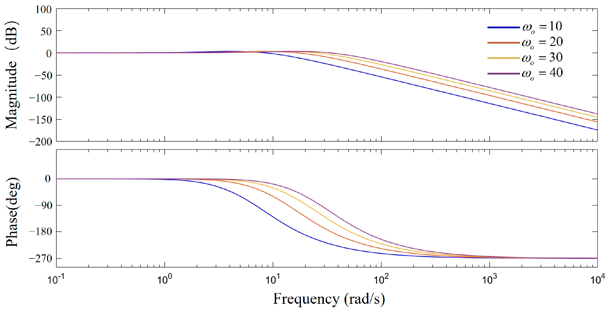
2.3. Design and Analysis of Continuous-Wave Pulse Generator LADRC

The purpose of LADRC is to transform the controlled object like Equation (9) into a linear integrator series standard type similar to $\ddot{y}=u_0$, so as to make the control simple [43]. The basic structure of LADRC is shown in Figure 4.

$$\ddot{y}=f\left(y,\dot{y},n,t,u\right)+b_{0}u$$

(9)

where $y$ is system output; $n$ is the disturbance signal; $u$ is the control signal; $f\left(y,\dot{y},n,t,u\right)$ is the total disturbance of the system which combines internal disturbance and external disturbance; and $b_0$ represents the known part of the gain of the control signal. Generally, $u=b_0^{-1}(u_0-z_3)$, and $z_3$ is LESO’s estimate of $f\left(y,\dot{y},n,t,u\right)$.

LADRC controller is built according to the PMSM mathematical model. First, we rewrite Equation (8) in the form of Equation (9), as shown in Equation (10).

$${\ddot{\theta }}_m=b_0{i}_q+f$$

(10)

where $b_0={\displaystyle \frac{3p_n{\phi }_f}{2J}}$; $f=-{\displaystyle \frac{\rho \xi \left(Q_s{v}_s\cos {\theta }_s-Q_{sr}{v}_{sr}\right)r+B{\omega }_m}{J}}$.

Then, based on Equation (10), the extended state space expression of the constructed system is

$$\left\{\begin{array}{l}{\dot{x}}_1=x_2\hfill \\ {\dot{x}}_2=x_3+b_{0}u\hfill \\ {\dot{x}}_3=\dot{f}\\ y=x_1\end{array}\right.$$

(11)

where $x_1={\theta }_m$; $x_2={\dot{\theta }}_m$; $x_3=f$; $u=i_q$.

Since $\dot{f}$ is unknown and can be estimated by LESO, ignoring $\dot{f}$ builds LESO as

$$\left\{\begin{array}{l}{e}_z=z_1-y\\ {\dot{z}}_1=-{\beta }_1{e}_z+z_2\\ {\dot{z}}_2=-{\beta }_2{e}_z+z_3+b_{0}u\hfill \\ {\dot{z}}_3=-{\beta }_3{e}_z\hfill \end{array}\right.$$

(12)

where $z_1$, $z_2$, and $z_3$ are LESO’s estimates of $x_1$, $x_2$, and $x_3$, respectively; $e_z$ is LESO’s estimation error of the system output; and ${\beta }_1$, ${\beta }_2$, and ${\beta }_3$ are the observer gains.

Finally, LSEF is constructed as Equation (13), and in order to simplify the parameter setting of LSEF, generally, $k_p={\omega }_c^2$ and $k_d=2{\omega }_c$, where ${\omega }_c$ is called the controller bandwidth.

$$u={\displaystyle \frac{k_p({\theta }_{ref}-{\mathrm{z}}_1)-k_d{z}_2-z_3}{b_0}}$$

(13)

where ${\theta }_{ref}$ is the system reference input signal.

The transfer function of the perturbation estimate $z_3$ and the total disturbance $f$ of the system can be obtained from Equations (10) and (12) as follows:

$${\displaystyle \frac{Z_3(s)}{F(s)}}={\displaystyle \frac{{\beta }_3}{s^3+{\beta }_1{s}^2+{\beta }_{2}s+{\beta }_3}}$$

(14)

To simplify the parameter setting of LESO so that the roots of the LESO characteristic equation $\lambda (s)$ are in the same position, that is, $\lambda (s)={(s+{\omega }_o)}^3$, the result can be ${\beta }_1=3{\omega }_o$, ${\beta }_2=3{\omega }_o^2$, and ${\beta }_3={\omega }_o^3$, where ${\omega }_o$ is called the observer bandwidth, and Equation (14) can be rewritten as

$${\displaystyle \frac{Z_3(s)}{F(s)}}={\displaystyle \frac{{\omega }_o^3}{{(s+{\omega }_o)}^3}}$$

(15)

When the total disturbance is a ramp signal, that is, $f(t)=kt$, the disturbance estimate $z_3$ can be expressed in the time domain by the inverse Laplace transform as follows:

$$z_3(t)={\displaystyle \frac{k{\omega }_o}{2}}{t}^2{e}^{-{\omega }_{o}t}+2kt{e}^{-{\omega }_{o}t}+{\displaystyle \frac{3k}{{\omega }_o}}{e}^{-{\omega }_{o}t}+kt-{\displaystyle \frac{3k}{{\omega }_o}}$$

(16)

Disturbance estimation error $e_f(t)=z_3(t)-f(t)$ of LESO can be expressed as Equation (17). From $\underset{t\to \infty }{\lim }{e}_f(t)=-{\displaystyle \frac{3k}{{\omega }_o}}$, it can be seen that there is always a steady-state error in LESO’s estimation of the total disturbance $f$, as shown in Figure 5, where Figure 5a describes LESO’s estimation of $f$ when $k=1$.

$$e_f(t)={\displaystyle \frac{k{\omega }_o}{2}}{t}^2{e}^{-{\omega }_{o}t}+2kt{e}^{-{\omega }_{o}t}+{\displaystyle \frac{3k}{{\omega }_o}}{e}^{-{\omega }_{o}t}-{\displaystyle \frac{3k}{{\omega }_o}}$$

(17)

Similarly, Figure 5b,c show LESO’s estimation of $f$ at $f(t)=t^2$ and $f(t)=t^3$, respectively. It can be seen from the figure that for nonlinear disturbance, the disturbance estimation error of LESO is larger, and the error keeps increasing as time changes.

As can be seen from Figure 5, when the observer bandwidth ${\omega }_o$ is low, LESO’s estimation of $f$ is not ideal. Although increasing ${\omega }_o$ can reduce the disturbance estimation error to a certain extent, the high-frequency amplitude–frequency characteristics of LESO will be increased, resulting in the noise robustness of the system being reduced, as shown in Figure 6.

Therefore, the estimation accuracy and noise robustness of LESO are inherently antagonistic. However, LESO, as a key link of LADRC, directly determines the performance of the control system. So, ILADRC will be presented later in this article. Firstly, CLESO is introduced to improve the accuracy of disturbance estimation. Then, an adaptive control law is proposed for the continuous-wave pulse generator, which further improves the control performance of the system.

3. ILADRC Policy

This section discusses the ILADRC algorithm, which mainly includes the following steps:

• CLESO;
• Adaptive control law;
• LSEF based on reduced-order LESO.

The structure diagram of the PMSM position servo system combined with the above links is shown in Figure 7.

3.1. CLESO

The basic idea of CLESO is to take LESO’s estimation of the total disturbance $z_3$ as the known input of the additional linear extended state observer (ALESO) and construct ALESO to estimate the residual disturbance. ALESO, as a supplement to LESO, can further reduce the impact of perturbations on the system. The estimate of the total disturbance by CLESO is the sum of one and the estimate of the residual disturbance by ALESO.

First, we rewrite Equation (10) to Equation (18)

$${\ddot{\theta }}_m=b_0{i}_q+z_3+g$$

(18)

where $g$ is the residual disturbance.

Then, we build ALESO as

$$\dot{v}=(A-L_{a}C)v+\left[\begin{array}{ccc}B& B_a& L_a\end{array}\right]u_a$$

(19)

where $A=\left[\begin{array}{ccc}0& 1& 0\\ 0& 0& 1\\ 0& 0& 0\end{array}\right]$; $B=\left[\begin{array}{c}0\\ b_0\\ 0\end{array}\right]$; $B_a=\left[\begin{array}{c}0\\ 1\\ 0\end{array}\right]$; $C=\left[\begin{array}{ccc}1& 0& 0\end{array}\right]$; $L_a=\left[\begin{array}{c}{\beta }_{a1}\\ {\beta }_{a2}\\ {\beta }_{a3}\end{array}\right]$; $u_a=\left[\begin{array}{c}u\\ z_3\\ y\end{array}\right]$; $v=\left[\begin{array}{c}{v}_1\\ v_2\\ v_3\end{array}\right]$; $v_1$, $v_2$ is ALESO’s estimate of $x_1$, $x_2$; $v_3$ is ALESO’s estimate of the residual disturbance $g$.

The roots of LSEO and ALESO characteristic equations are unified to ${\omega }_{ao}$, that is, $L=L_a={\left[\begin{array}{ccc}3{\omega }_{ao}& 3{\omega }_{ao}^2& {\omega }_{ao}^3\end{array}\right]}^T$; ${\omega }_{ao}$ is the observer bandwidth of cascading LADRC. LSEF based on CLESO can be described as Equation (20). Since the mechanical Angle and speed of the PMSM rotor of the continuous-wave pulse generator can be obtained by the sensor, the CLESO is reduced by two steps, that is, the CLESO only outputs $z_3$ and $v_3$, and the LSEF can be simplified to Equation (21).

$$u={\displaystyle \frac{k_p({\theta }_{ref}-z_1)-k_d{z}_2-z_3-v_3}{b_0}}$$

(20)

$$u={\displaystyle \frac{k_p({\theta }_{ref}-{\theta }_m)-k_d{\omega }_m-z_3-v_3}{b_0}}$$

(21)

where $k_p={\omega }_c^2$, $k_d=2{\omega }_c$, and ${\theta }_m$ and ${\omega }_m$ are the mechanical Angle and mechanical angular velocity of the PMSM rotor.

From Equations (10), (15), and (19), the transfer function of the ALESO disturbance estimate $v_3$ and the total disturbance $f$ can be obtained, as shown in Equation (22). The transfer function of the CLESO disturbance estimate $z_3+v_3$ and the total disturbance $f$ is shown in Equation (23).

$${\displaystyle \frac{v_3(s)}{f(s)}}={\displaystyle \frac{{\beta }_{a3}(s^3+{\beta }_{a1}{s}^2+{\beta }_{a2}s)}{{(s^3+{\beta }_{a1}{s}^2+{\beta }_{a2}s+{\beta }_{a3})}^2}}={\displaystyle \frac{{\omega }_{ao}^3(s^3+3{\omega }_{ao}{s}^2+3{\omega }_{ao}^{2}s)}{{(s+{\omega }_{ao})}^6}}$$

(22)

$${\displaystyle \frac{z_3(s)+v_3(s)}{f(s)}}={\displaystyle \frac{{\omega }_{ao}^3}{{(s+{\omega }_{ao})}^3}}+{\displaystyle \frac{{\omega }_{ao}^3(s^3+3{\omega }_{ao}{s}^2+3{\omega }_{ao}^{2}s)}{{(s+{\omega }_{ao})}^6}}$$

(23)

When the disturbance $f(t)=kt$, $v_3$ can be expressed as Equation (24) in the time domain, and the disturbance estimation error $e_{af}(t)=z_3(t)+v_3(t)-f(t)$ of the CLESO can be obtained from Equations (16) and (24), which is expanded as Equation (25). It can be seen from $\underset{t\to \infty }{\lim }{e}_{af}(t)=0$ that when the disturbance is a slope function, there is no steady-state error in the estimation of the total disturbance by CLESO, as shown in Figure 8, where Figure 8a describes the estimation of CLESO to $f$ when $k=1$.

$$v_3(t)=-k{e}^{-{\omega }_{ao}t}[{\displaystyle \frac{{\omega }_{ao}^4}{120}}{t}^5+{\displaystyle \frac{2{\omega }_{ao}^3}{24}}{t}^4+{\displaystyle \frac{3{\omega }_{ao}^2}{6}}{t}^3+{\displaystyle \frac{3{\omega }_{ao}}{2}}{t}^2+3t+{\displaystyle \frac{3}{{\omega }_{ao}}}]+{\displaystyle \frac{3k}{{\omega }_{ao}}}$$

(24)

$$e_{af}(t)=-k{e}^{-{\omega }_{ao}t}[{\displaystyle \frac{{\omega }_{ao}^4}{120}}{t}^5+{\displaystyle \frac{2{\omega }_{ao}^3}{24}}{t}^4+{\displaystyle \frac{3{\omega }_{ao}^2}{6}}{t}^3+{\omega }_{ao}{t}^2+t]$$

(25)

Similarly, when the perturbations are nonlinear functions $f(t)=t^2$ and $f(t)=t^3$, the estimation of the perturbations by CLESO is shown in Figure 8b,c. Under the condition of the same observer bandwidth, the disturbance tracking error of CLESO is significantly smaller than that of traditional LESO compared with Figure 5. The disturbance estimation error of CLESO at 1 s is generally less than 50% of the estimation error of LESO. Therefore, LADRC based on CLESO can estimate and eliminate the total disturbance more thoroughly and has stronger anti-disturbance performance.

3.2. Adaptive LSEF Control Strategy

For low-order systems, the introduction of ${\omega }_c$ to reduce the number of LSEF parameters can enhance the dynamic response performance of the system and improve the transmission rate of the pulse generator. However, the continuous-wave pulse generator requires the PMSM rotor to reverse frequently, and due to the moment of inertia of the shear valve rotor, too fast response speed will lead to a large overshoot and reduce the system stability margin. Although reducing ${\omega }_c$ can improve the stability of the system, it also makes the system less responsive. In addition, when the system order is greater than the first order, ${\omega }_c$ cannot cover all the value ranges of LSEF parameters, such as Equation (21); ${\omega }_c$ cannot represent all the values of $k_p$ and $k_d$; and it is difficult to achieve ideal parameter tuning only by adjusting ${\omega }_c$.

To reduce the overshoot of the continuous-wave pulse generator and improve the response speed and stability of the system, a new adaptive control law is proposed, which consists of two parts: the adaptive law based on periodic wave response and the adaptive law based on tracking error. The adaptive control law can dynamically adjust $k_p$ and $k_d$ parameters. The new adaptive control law is shown below.

$$\left\{\begin{array}{c}{k}_p=k_{pw}+\eta k_{pe}\\ k_d=k_{dw}+\eta k_{de}\end{array}\right.$$

(26)

where $k_{pw}$ and $k_{dw}$ are the parameters based on the adaptive law of periodic wave response; $k_{pe}$ and $k_{de}$ are the parameters based on the adaptive law of tracking error; and $\eta$ is the gain based on the adaptive law of tracking error.

Equation (27) defines the tracking error $e_{\theta }$ and the range ${\chi }_p$ and ${\chi }_d$ for $k_p$ and $k_d$.

$$\left\{\begin{array}{l}{e}_{\theta }={\theta }_{ref}-{\theta }_m\hfill \\ {\chi }_p=k_{p\max }-k_{p\min }\hfill \\ {\chi }_d=k_{d\max }-k_{d\min }\hfill \end{array}\right.$$

(27)

where $k_{p\max }$ and $k_{p\min }$, and $k_{d\max }$ and $k_{d\min }$ are the maximum and minimum values of $k_p$ and $k_d$, respectively.

As shown in Figure 9, the QPSK modulation waveform requires the PMSM rotor to swing frequently in a sinusoidal waveform. In the area marked red in the figure, a large tracking error will cause the controller to produce a large output. When the system response is near the extreme value, the tracking error will decrease rapidly, and the controller output will also decrease. However, due to the existence of a moment of inertia, the system is difficult to react quickly, so the controller can easily cause a system overshoot harmonic oscillation by relying only on the error. To solve this problem, an adaptive law based on periodic wave response is proposed. The basic idea is to reduce the output of the controller within this time interval before the system response reaches the extreme point (red marked area in Figure 9), and at the same time, increase the output of the controller after the system response reaches the extreme point to make the system respond quickly.

Combined with Equation (27), the adaptive law based on periodic wave response can be described as Equations (28) and (29).

$$k_{pw}=\left\{\begin{array}{ll}{\displaystyle \frac{{\chi }_p}{\pi }}\arctan {\epsilon }_{pw}(||{\theta }_m|-\delta |-{\sigma }_{pw})+{\displaystyle \frac{{\chi }_p}{2}}+k_{p\min },\hfill & |{\theta }_m(t_{now})|\ge |{\theta }_m(t_{last})|\\ k_{p\max },\hfill & |{\theta }_m(t_{now})|<|{\theta }_m(t_{last})|\end{array}\right.$$

(28)

$$k_{dw}=\left\{\begin{array}{ll}{\displaystyle \frac{{\chi }_p}{\pi }}\arctan {\epsilon }_{dw}({\displaystyle \frac{1}{\left|\right|{\theta }_m|-\delta |}}-{\sigma }_{dw})+{\displaystyle \frac{{\chi }_p}{2}}+k_{p\min },\hfill & |{\theta }_m(t_{now})|\ge |{\theta }_m(t_{last})|\\ k_{d\max },\hfill & |{\theta }_m(t_{now})|<|{\theta }_m(t_{last})|\end{array}\right.$$

(29)

where ${\epsilon }_{pw}$ and ${\epsilon }_{dw}$, $\delta$, and ${\sigma }_{pw}$ and ${\sigma }_{dw}$ are the parameters based on the adaptive law of periodic wave response; ${\theta }_m(t_{now})$ is the current output of the controlled object; and ${\theta }_m(t_{last})$ is the output of the controlled object at the last moment.

The influence of ${\epsilon }_{pw}$ and ${\epsilon }_{dw}$, $\delta$, and ${\sigma }_{pw}$ and ${\sigma }_{dw}$ on $k_{pw}$ and $k_{dw}$ can be described in Figure 10, as shown in Figure 10a; with the increase in ${\sigma }_{pw}$ or the decrease in ${\sigma }_{dw}$, the interval of $k_{pw}\approx k_{p\min }$ and $k_{dw}\approx k_{d\max }$ keeps expanding. As shown in Figure 10b, ${\epsilon }_{pw}$ and ${\epsilon }_{dw}$ affect the sensitivity of $k_{pw}$ and $k_{dw}$ to ${\theta }_m$. The smaller ${\epsilon }_{pw}$ and ${\epsilon }_{dw}$ are, the smoother the adaptive law curve based on periodic wave response is. Figure 10c shows the influence of $\delta$, as it can be seen that $\delta$ determines where $k_{pw}$ goes down and $k_{dw}$ goes up.

The adaptive law based on periodic fluctuation response is not sensitive to the change in tracking error, so the system response cannot reach the set value near the extreme point, and so the adaptive law based on tracking error is proposed to compensate.

Combined with Equation (27), the adaptive law based on tracking error can be described as Equation (30).

$$k_{dw}=\left\{\begin{array}{ll}{\displaystyle \frac{{\chi }_p}{\pi }}\arctan {\epsilon }_{dw}({\displaystyle \frac{1}{\left|\right|{\theta }_m|-\delta |}}-{\sigma }_{dw})+{\displaystyle \frac{{\chi }_p}{2}}+k_{p\min },\hfill & |{\theta }_m(t_{now})|\ge |{\theta }_m(t_{last})|\\ k_{d\max },\hfill & |{\theta }_m(t_{now})|<|{\theta }_m(t_{last})|\end{array}\right.$$

(30)

where ${\epsilon }_{pe}$ and ${\epsilon }_{de}$, and ${\sigma }_{pe}$ and ${\sigma }_{de}$ are parameters based on the adaptive law of tracking error.

The behavior of $k_{pe}$ and $k_{de}$ exhibits an inverse relationship: as $e_{\theta }$ gradually increases, $k_{pe}$ increases while $k_{de}$ decreases; conversely, as $e_{\theta }$ decreases, $k_{pe}$ decreases and $k_{de}$ increases. The impact of each parameter on the adaptive law is illustrated in Figure 11. From Figure 11a, it can be observed that as ${\sigma }_{pe}$ increases and ${\sigma }_{de}$ decreases, the range where $k_{pe}\approx k_{p\min }$ and $k_{de}\approx k_{d\max }$ expands. Figure 11b demonstrates that ${\epsilon }_{pe}$ and ${\epsilon }_{de}$ influence the sensitivity of $k_{pe}$ and $k_{de}$ to changes in $e_{\theta }$; as ${\epsilon }_{pe}$ and ${\epsilon }_{de}$ decrease, the adaptive curves of $k_{pe}$ and $k_{de}$ gradually become more linear. According to Equation (21), when $e_{\theta }$ increases, changes in $k_p$ and $k_d$ lead to an increase in the controller’s output and a faster system response; when $e_{\theta }$ decreases, the controller’s output diminishes.

4. Simulation Verification

4.1. Simulation Setup

The PMSM position servo system typically consists of a current loop, a speed loop, and a position loop. The current and speed loops generally use PI controllers, while the position loop commonly employs a P controller or other types of controllers.

In this study, the simulation models of the position servo control system for the oscillating continuous-wave pulse generator PMSM were constructed using both a P controller and a LADRC controller in the position loop. The speed and current loops were controlled using PI controllers, as illustrated in Figure 12.

Additionally, a simulation model of the position servo control system based on the ILADRC controller was developed. Since ILADRC is a second-order controller, the speed loop is omitted. The current loop is controlled using a PI controller, as shown in Figure 7.

Using the simulation models, we analyzed and compared the load disturbance rejection capabilities and noise robustness of the P, LADRC, and ILADRC controllers in the position loop. Furthermore, a QPSK signal modulation method was employed to simulate actual operating conditions, where the transmission frequency was set to 20 bit/s, and the double-bit code elements “00 00” and “01 10” were used. The motor rotor’s oscillation range was set to [−15°, +15°] (radians: [−0.262, +0.262]). The system input waveform is shown in Figure 13.

Figure 14 shows the experimental platform for the continuous-wave pulse generator. The simulation was conducted using the actual parameters of the surface-mounted PMSM from this experimental platform, as listed in

Table 1. Table mount three-phase PMSM parameters.

Parameters	Value	Parameters	Value
Bus voltage (V)	90	Rated speed (r/min)	520
Rated current (A)	4.15	Maximum current (A)	8.5
Rated torque (Nm)	4.72	Peak torque (Nm)	9.62
Torque coefficient (Nm/A)	1.137	Permanent magnet flux linkage (Wb)	0.28425
Phase resistance ($\Omega$)	2.03	Phase inductance (H)	$4.45\times {10}^{-3}$
Total inertia ($\mathrm{Kg}\times {\mathrm{m}}^2$)	$4.12\times {10}^{-4}$

. The simulation was performed on an Intel 12th generation Core i5-12400 six-core CPU (Intel, Santa Clara, CA, USA) with 32 GB DDR4 3200 MHz RAM (16 GB + 16 GB) (King Bank, Shenzhen, China) and an NVIDIA GeForce RTX 3060Ti GPU (GAINWARD, Shenzhen, China).

During the simulation, the parameter settings for the PMSM position servo system based on the P and LADRC strategies are provided in

Table 2. Parameters of PMSM position servo system based on position loop P control strategy.

Controller	Parameters	Value
Current loop PI	$K_{ep}$	8
	$K_{ei}$	50
Velocity loop PI	$K_{vp}$	0.1
	$K_{vi}$	2.83
Position loop P	$K_{\theta p}$	2000

and

Table 3. Parameters of PMSM position servo system based on position loop LADRC strategy.

Controller	Parameters		Value
Current loop PI	$K_{ep}$		8
	$K_{ei}$		50
Velocity loop PI	$K_{vp}$		0.1
	$K_{vi}$		2.83
Position loop LADRC	LSEF	$k_p$	$7\times {10}^5$
		$k_d$	200
		$b_0$	4140
	LESO	${\omega }_o$	1200

, respectively. The parameters for the PMSM position servo system based on the ILADRC strategy are shown in

Table 4. Parameters of PMSM position servo system based on ILADRC strategy.

Controller	Parameters		Value
Current loop PI		$K_{ep}$	8
		$K_{ei}$	50
Position loop ILADRC	Adaptive law	${\chi }_p$	$[1\times {10}^5$$, 7\times {10}^5$]
		${\chi }_d$	[230, 370]
		$\eta$	1
		$[{\sigma }_{pw}$, ${\sigma }_{dw}$, ${\epsilon }_{pw}$, ${\epsilon }_{dw}$, $\delta$]	[100 1 0.02 30 0.262]
		$[{\sigma }_{pw}$$, {\sigma }_{dw}$$, {\epsilon }_{pw}$$, {\epsilon }_{dw}$]	[20 0.05 0.04 30]
	LSEF	$b_0$	4140
	LESO	${\omega }_o$	1200

. All the parameters in Table 2, Table 3 and Table 4 are the results of fine-tuning. To ensure a fair comparison, the parameters of the PI controllers in the current loops are kept consistent across all three control strategies. Additionally, the value of $b_0$ in both LADRC and ILADRC is set to be the same, and the observer bandwidths are matched (${\omega }_0={\omega }_{su0}$).

4.2. Simulation Result Analysis

Figure 15 analyzes the effects of abrupt loads on the different controllers. The PMSM Angle is controlled at 0.262 rad (i.e., 15°), then the load torque of $2\mathrm{N}·\mathrm{m}$ is applied to the PMSM at 0.05 s, and the anti-abrupt load performance of the position loop P control, LADRC, and ILADRC is compared. As shown in Figure 15a, the maximum angular fluctuation controlled by P is $5.5\times {10}^{-3}$ rad, and the duration of the fluctuation is 100 ms. The maximum angular fluctuation of LADRC is $4.5\times {10}^{-3}$ rad, but the fluctuation duration is only 10 ms. The maximum angular fluctuation of ILADRC is $2.5\times {10}^{-3}$ rad, which is only 45% of the P control and 55% of the LADRC, and the fluctuation duration is 8 ms, which is 80% of the LADRC. Figure 15b and Figure 15c describe the change process of the control signal $u$ and the adaptive law parameters. It can be seen from Figure 15b that when PMSM is just subjected to load torque, $k_p$ increases, $k_d$ decreases, and $u$ increases rapidly. When $u$ reaches its maximum value, $k_p$ decreases and $k_d$ increases, and $u$ quickly stays near 0.5. The oscillations of $k_p$ and $k_d$ in the whole process are caused by the low sampling rate of the system and the large curvature of the adaptive law curve. In addition, since the load torque has little effect on the system response, the error-based adaptive law has little effect on $k_p$ and $k_d$, as shown in Figure 15c.

Figure 16 and Figure 17 analyze the tracking results of the different controllers for QPSK waveforms with input “00 00” and “01 10”. In the simulation process, the hydraulic torque received by PMSM in the well was simulated as the load torque with amplitude $2\mathrm{N}·\mathrm{m}$, phase, and frequency the same as the motion law of the shear valve rotor, as shown in Figure 16b and Figure 17b.

In Figure 16a, at the peak of the system response, the overshoot of P and LADRC is 0.04 rad and 0.031 rad, while the overshoot of ILADRC is 0.01 rad, which is only 25% of the P control and 32% of the LADRC. The lag time of the extreme point of the P control and LADRC is 3 ms and 4.5 ms, respectively, while the lag time of the ILADRC is 2 ms, which is only 67% of the P control and 44% of the LADRC. Figure 16c shows the process of $k_p$ and $k_d$ adjustment by ILADRC’s adaptive law. It can be seen from the figure that when ILADRC’s response approaches the peak and peak valley, $k_p$ decreases and $k_d$ increases, and the absolute value of ILADRC’s output, that is, $\left|u\right|$ decreases rapidly and system overshoot is inhibited. $k_p$ and $k_d$ recover to the maximum and minimum values, respectively; $\left|u\right|$ increases rapidly; and the system response speed increases.

As shown in Figure 17a, the phase of the “01 10” QPSK waveform changes between 0.08 s and 0.13 s. The phase conversion begins at 0.1 s, where the overshoot controlled by P is 0.03 rad. The overshoot of LADRC is increased to 0.08 rad, which is 2.5 times higher than that of the constant phase, and the lag time of the extreme point is increased by 1.3 times. The overshoot of ILADRC is still 0.01 rad. Compared with Figure 16a, the overshoot of ILADRC is not affected by the phase change. The lag time of the extreme point of P control and LADRC is 4 ms and 6 ms, respectively, while the lag time of the extreme point of ILADRC is still 2 ms. Figure 17c shows the process of adjusting $k_p$ and $k_d$ for ILADRC’s adaptive law. When the phase changes between 0.1 s and 0.11 s, $k_{p\mathrm{e}}$ and $k_{d\mathrm{e}}$ change amplitude decreases due to a small error and $\left|u\right|$ does not rise rapidly. Therefore, the system response speed of ILADRC is slightly slower than that of LADRC at phase change.

5. Conclusions

This paper presents ILADRC, which is applied to a continuous-wave pulse generator PMSM position servo control. By introducing CLESO and adaptive law, the control precision and response speed of the system are improved, and the overshoot of the system is reduced. To prove the superiority of ILADRC, the tracking results of QPSK modulation waveform by position loop P control, LADRC, and ILADRC are compared and analyzed. The following are the main findings and contributions of this paper:

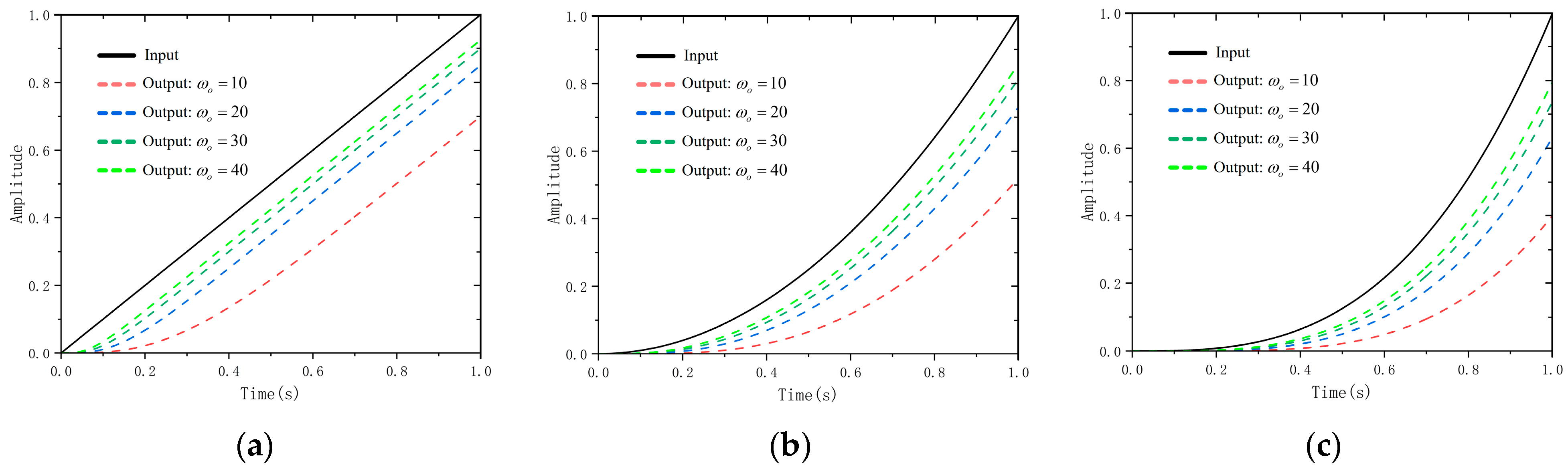
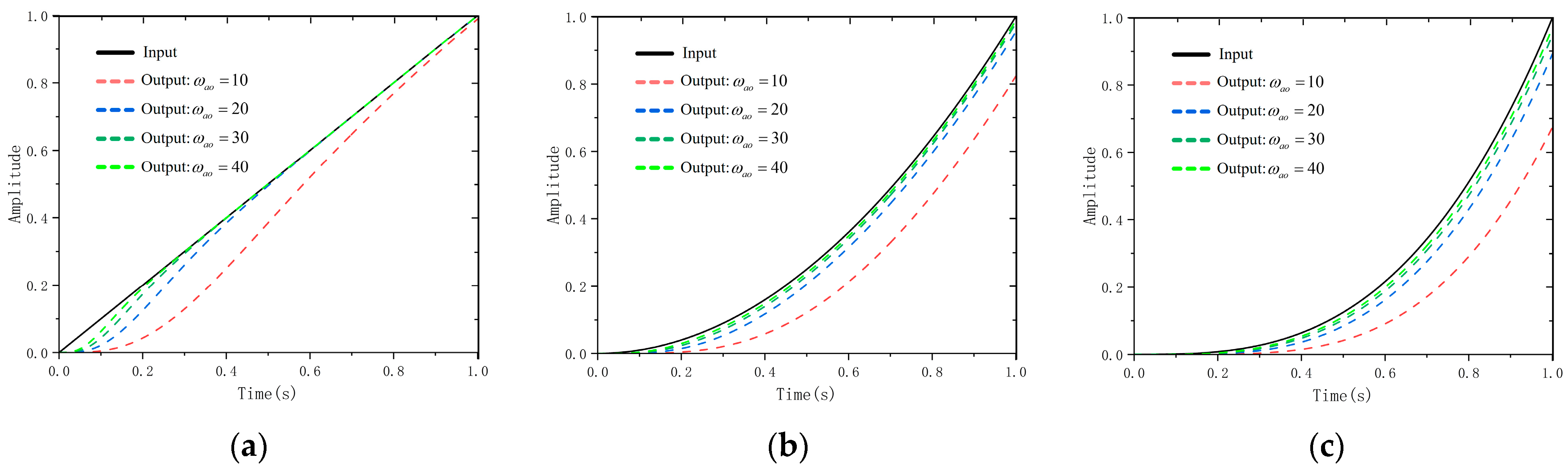
• The research shows that the traditional LESO estimation of step disturbance always has a steady-state error, and the estimation error of nonlinear disturbance cannot be convergent. At the same time, the contradiction between the estimation accuracy of LESO and the robustness of noise is revealed by analyzing the Bode diagram of LESO. Therefore, CLESO is introduced, and the simulation results show that CLESO can completely track slope disturbance signals, and the accuracy of nonlinear disturbance estimation is higher than that of the traditional LESO.
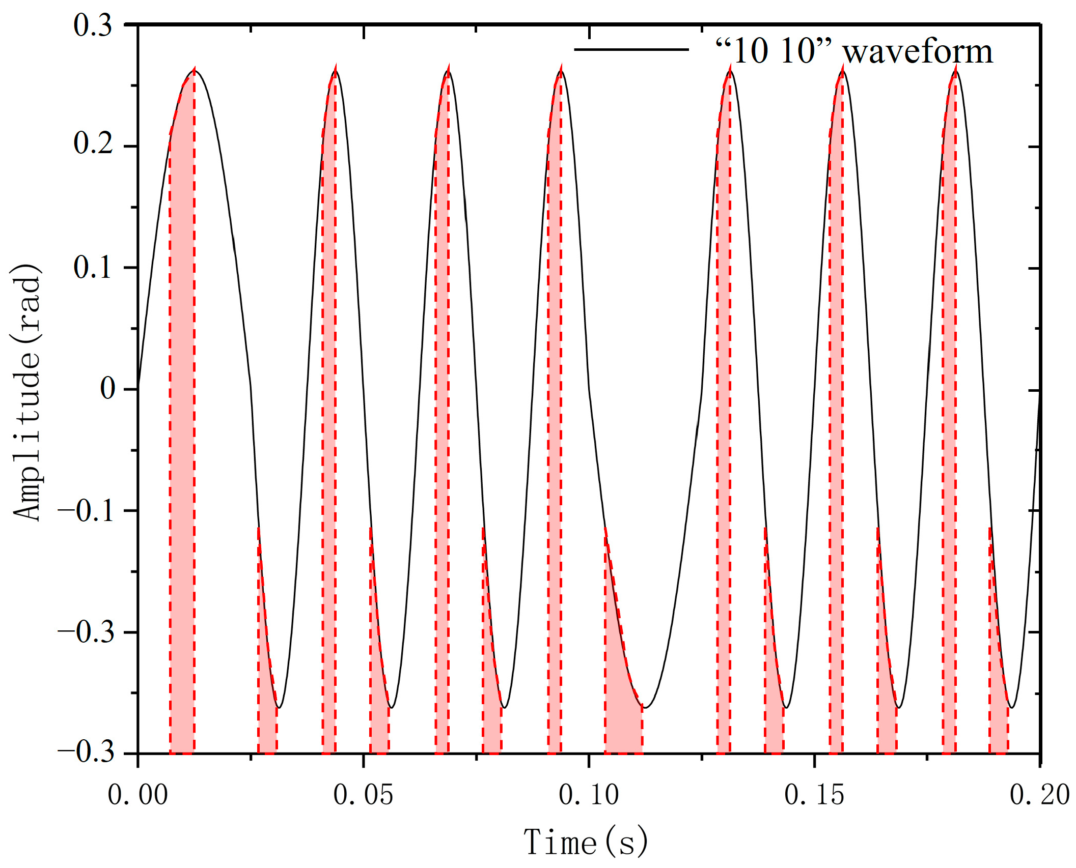
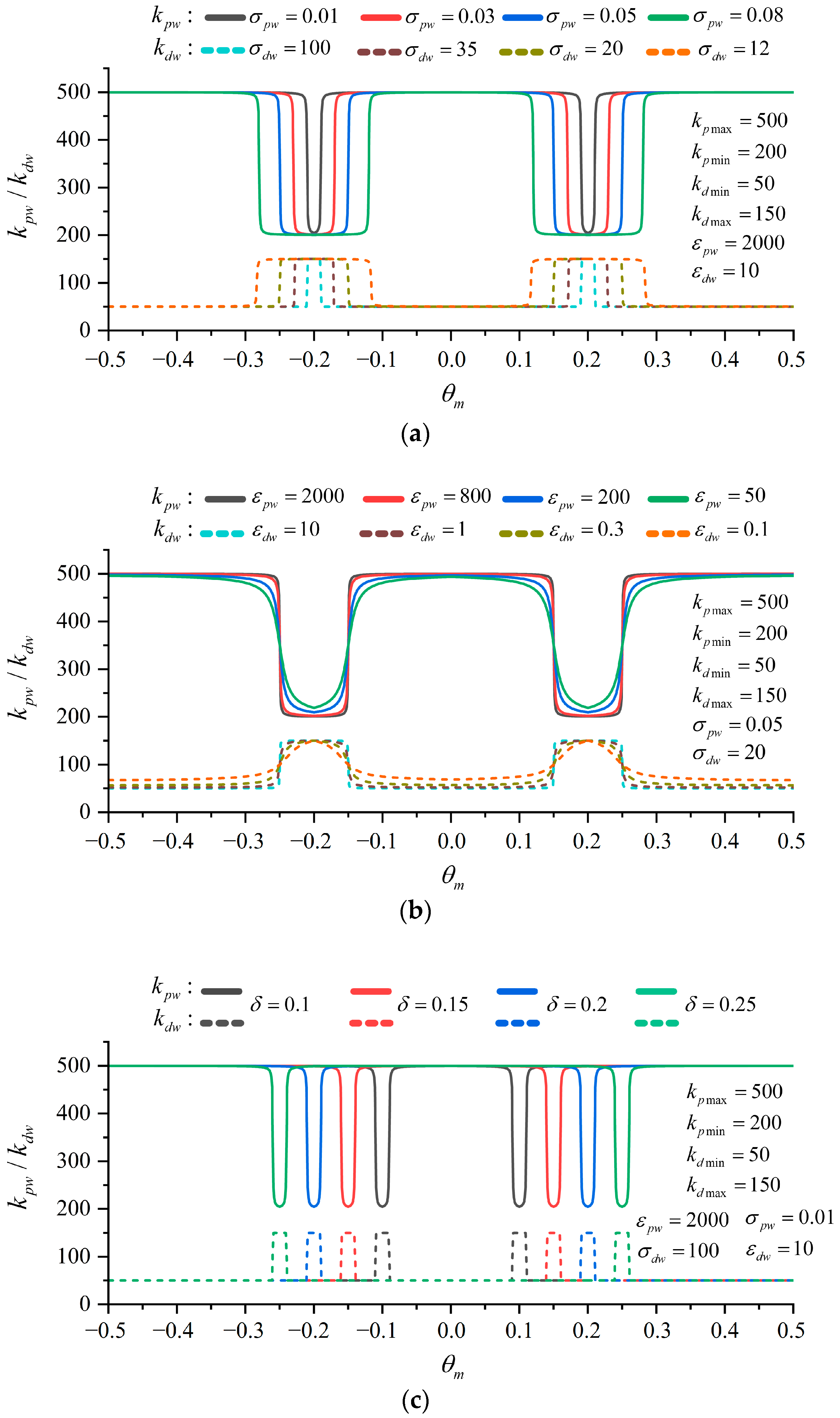
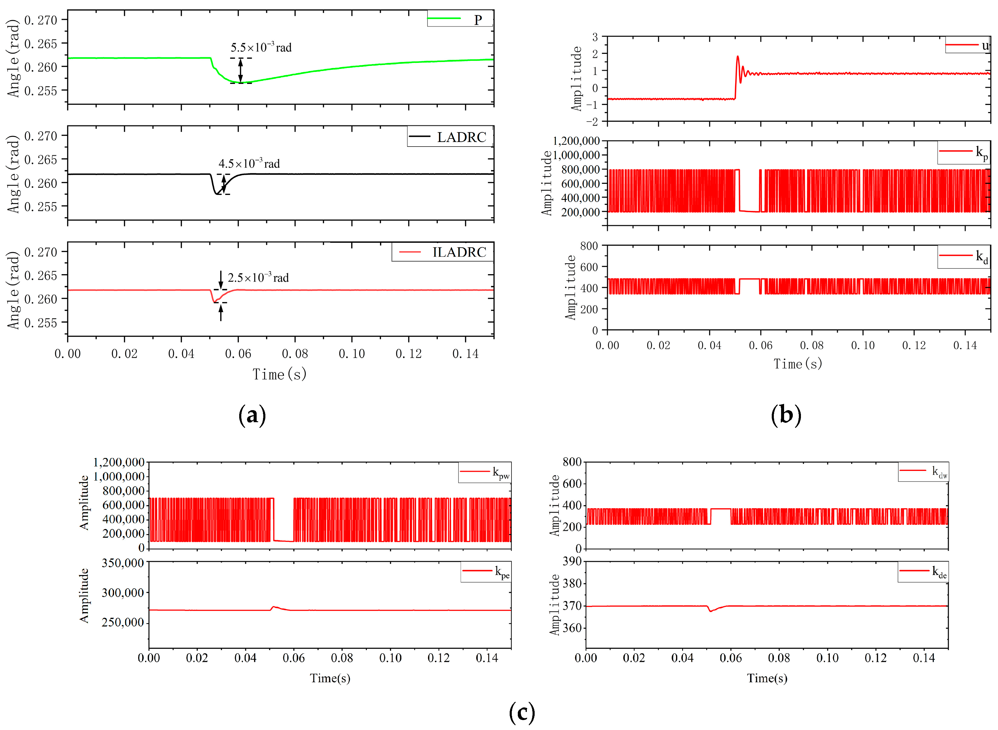
• By analyzing the response curve of an oscillating continuous-wave pulse generator, it is found that large controller output will lead to an overshoot of the system. Therefore, an adaptive LSEF control strategy is proposed, which consists of three parts: adaptive law based on periodic wave response, adaptive law based on tracking error and LSEF, and the influence of different adaptive law parameters on $k_p$ and $k_d$ is given.
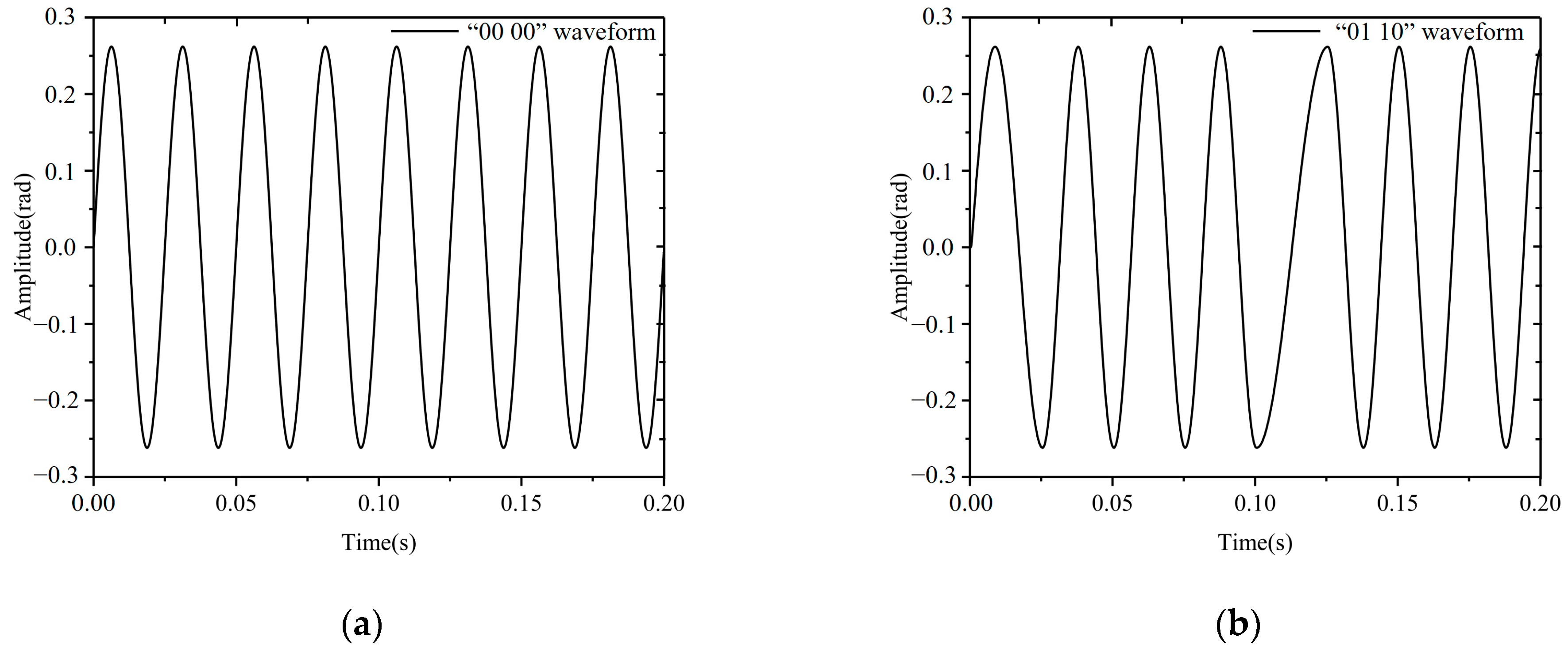
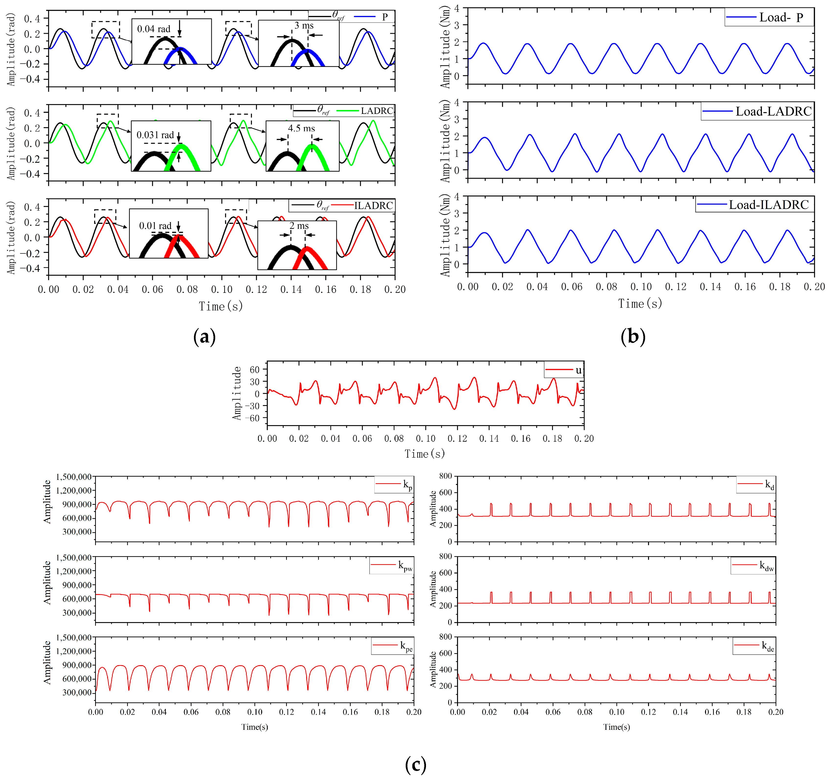
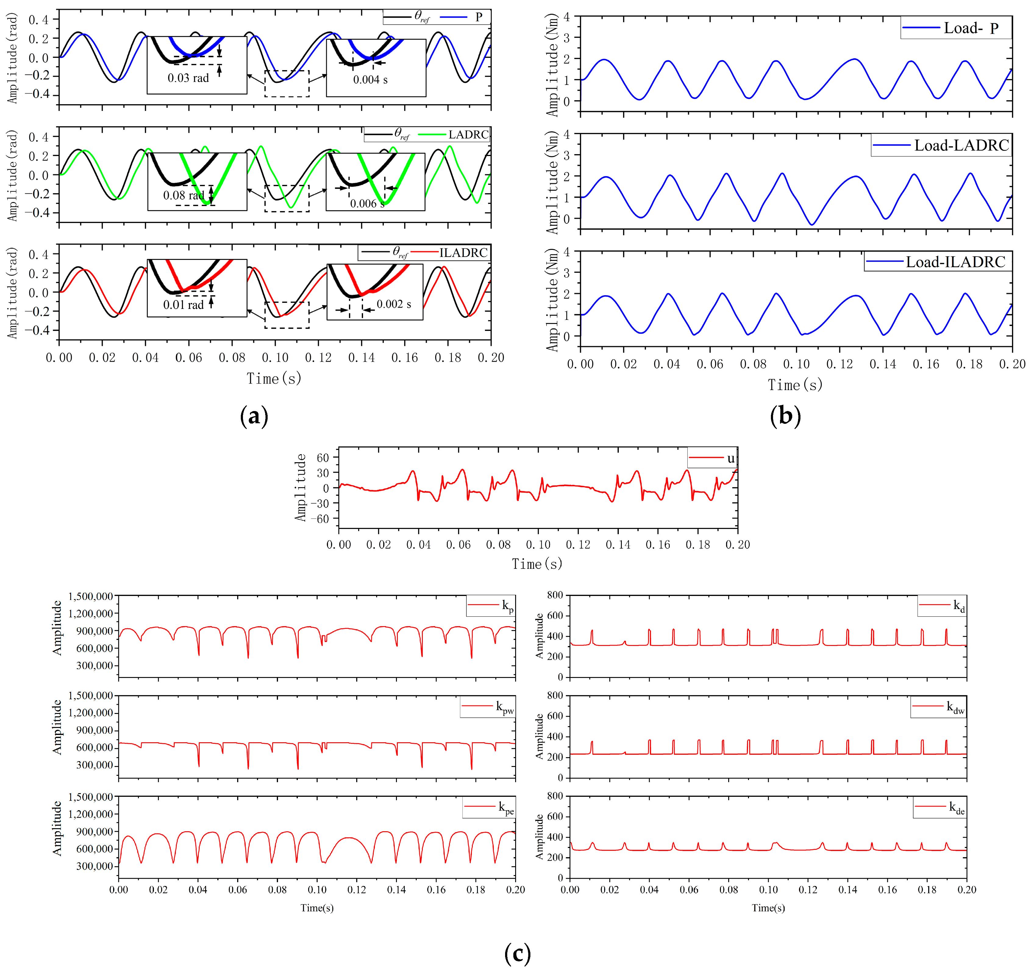
• The simulation results show that ILADRC has better anti-mutation load performance when the mutation load is $2\mathrm{N}·\mathrm{m}$. In addition, with the QPSK modulation method, ILADRC is superior to P control and LADRC in response speed and overshoot suppression at the transmission rate of 20 bit/s and QPSK phase invariant. At the same time, when the phase of the QPSK waveform changes, compared with the performance of LADRC, the control performance of ILADRC is not affected, and the overshoot and extreme point lag time do not change. However, due to the small tracking error, the adaptive law failed to adjust $k_{pe}$ and $k_{de}$ to maximize the controller output, so the system response speed decreased slightly.

How to improve the adaptive law so that the system response is not affected by the phase change in QPSK waveform is the future research direction; in addition, the complex control strategy will reduce the stability and reliability of the system, which is one of the limitations of ILADRC. It is hoped that this paper can provide more ideas for the practical application and analysis of oscillating continuous-wave pulse generators.

References

1. Gabriel, B.; Diego, B. Physics-Based Observers for Measurement-While-Drilling System in Down-the-Hole Drills. Available online: https://www-mdpi-com-s.vpn.ysu.edu.cn:8118/2227-7390/10/24/4814 (accessed on 18 July 2024).
2. Song, H.; Huang, H.; Zhang, J.; Qu, D. A New Measurement-While-Drilling System Based on Inertial Technology. Adv. Mech. Eng. 2018, 10, 1687814018767498. [Google Scholar] [CrossRef]
3. Qu, J.; Xue, Q. Analysis on the Change Characteristics of Waveform during the Transmission of Continuous Wave Mud Pulse Signal. Alex. Eng. J. 2023, 80, 594–608. [Google Scholar] [CrossRef]
4. Yan, Z.; Wang, Z.; Yang, N.; Pan, W.; Gao, T. Investigation on the Novel Unsteady-Liquid Thin-Walled Cutting-Edge Throttling Mechanism Incorporated in the Rotary Valve Design for a Continuous Wave Pulse Generator. Geoenergy Sci. Eng. 2024, 235, 212680. [Google Scholar] [CrossRef]
5. Zaihidee, F.M.; Mekhilef, S.; Mubin, M. Fractional Order PID Sliding Mode Control for Speed Regulation of Permanent Magnet Synchronous Motor. J. Eng. Res. 2021, 9, 209–218. [Google Scholar] [CrossRef]
6. Li, D.; Xiong, X.; Zhang, G.; Zhang, Y.; Zuo, R.; Feng, W. The Research on Sensorless Control of Permanent Magnet Synchronous Using SMC and SMO. IOP Conf. Ser. Mater. Sci. Eng. 2020, 717, 012019. [Google Scholar] [CrossRef]
7. Zou, M. Command Filtering-Based Adaptive Fuzzy Control for Permanent Magnet Synchronous Motors with Full-State Constraints. Inf. Sci. 2020, 518, 1–12. [Google Scholar] [CrossRef]
8. Yang, N.; Zhang, S.; Li, X.; Li, X. A New Model-Free Deadbeat Predictive Current Control for PMSM Using Parameter-Free Luenberger Disturbance Observer. IEEE J. Emerg. Sel. Top. Power Electron. 2023, 11, 407–417. [Google Scholar] [CrossRef]
9. Liu, P.; Cui, Y.; Wang, C.; Liang, Y.; Chang, Z.; Han, K.; Shen, S.; Zuo, G. Sensorless Model Predictive Control Based on I-f Integrated Sliding Mode Observer for Surface Permanent Magnet Synchronous Motor. Int. J. Circuit Theory Appl. 2024, 52, 934–953. [Google Scholar] [CrossRef]
10. Feng, Y. Chattering Free Full-Order Sliding-Mode Control. Automatica 2014, 50, 1310–1314. [Google Scholar] [CrossRef]
11. Precup, R.E. A Survey on Fuzzy Control for Mechatronics Applications. Available online: https://www-tandfonline-com-s.vpn.ysu.edu.cn:8118/doi/full/10.1080/00207721.2023.2293486 (accessed on 15 July 2024).
12. Hu, Z. Model-Free Predictive Control of Motor Drivers and Power Converters: A Review |IEEE Journals and Magazines |IEEE Xplore (IEEE Xplore). Available online: https://ieeexplore-ieee-org-s.vpn.ysu.edu.cn:8118/document/9492066 (accessed on 15 July 2024).
13. Huang, Y.; Xue, W. Active Disturbance Rejection Control: Methodology and Theoretical Analysis. ISA Trans. 2014, 53, 963–976. [Google Scholar] [CrossRef]
14. Rsetam, K.; Al-Rawi, M.; Cao, Z. Robust Adaptive Active Disturbance Rejection Control of an Electric Furnace Using Additional Continuous Sliding Mode Component. ISA Trans. 2022, 130, 152–162. [Google Scholar] [CrossRef] [PubMed]
15. Wu, Z.; Shi, G.; Li, D.; Liu, Y.; Chen, Y. Active Disturbance Rejection Control Design for High-Order Integral Systems. ISA Trans. 2022, 125, 560–570. [Google Scholar] [CrossRef]
16. Wang, L.; Wang, X.; Liu, G.; Li, Y. Improved Auto Disturbance Rejection Control Based on Moth Flame Optimization for Permanent Magnet Synchronous Motor. IEEJ Trans. Electr. Electron. Eng. 2021, 16, 1124–1135. [Google Scholar] [CrossRef]
17. Zhang, X.; Chen, Y.; Sun, X. Overview of Active Disturbance Rejection Control for Permanent Magnet Synchronous Motors. J. Electr. Eng. Technol. 2024, 19, 1237–1255. [Google Scholar] [CrossRef]
18. Wang, B.; Tian, M.; Yu, Y.; Dong, Q.; Xu, D. Enhanced ADRC With Quasi-Resonant Control for PMSM Speed Regulation Considering Aperiodic and Periodic Disturbances. IEEE Trans. Transp. Electrif. 2022, 8, 3568–3577. [Google Scholar] [CrossRef]
19. Liu, C.; Luo, G.; Chen, Z.; Tu, W. Measurement Delay Compensated LADRC Based Current Controller Design for PMSM Drives with a Simple Parameter Tuning Method. ISA Trans. 2020, 101, 482–492. [Google Scholar] [CrossRef] [PubMed]
20. Wang, Z.; Wang, Y.; Cai, Z.; Zhao, J.; Liu, N.; Zhao, Y. Unified Accurate Attitude Control for Dual-Tiltrotor UAV with Cyclic Pitch Using Actuator Dynamics Compensated LADRC. Sensors 2022, 22, 1559. [Google Scholar] [CrossRef]
21. Cai, Z.; Wang, Z.; Zhao, J.; Wang, Y. Equivalence of LADRC and INDI Controllers for Improvement of LADRC in Practical Applications. ISA Trans. 2022, 126, 562–573. [Google Scholar] [CrossRef]
22. Zhao, M.; Hu, Y.; Song, J. Improved Fractional-Order Extended State Observer-Based Hypersonic Vehicle Active Disturbance Rejection Control. Mathematics 2022, 10, 4414. [Google Scholar] [CrossRef]
23. Ying, Z. A Variable Parameter Method Based on Linear Extended State Observer for Position Tracking. Available online: https://www-mdpi-com-s.vpn.ysu.edu.cn:8118/2076-0825/11/2/41 (accessed on 15 July 2024).
24. Zhang, J. Robust and Adaptive Backstepping Control for Hexacopter UAVs |IEEE Journals and Magazines |IEEE Xplore (IEEE Xplore). Available online: https://ieeexplore-ieee-org-s.vpn.ysu.edu.cn:8118/document/8890948 (accessed on 15 July 2024).
25. Xu, Q. Low-Speed LADRC for Permanent Magnet Synchronous Motor with High-Pass Speed Compensator. Available online: https://ieeexplore-ieee-org-s.vpn.ysu.edu.cn:8118/document/10292603 (accessed on 15 July 2024).
26. Pan, Z.; Wang, X.; Zheng, Z.; Tian, L. Fractional-Order Linear Active Disturbance Rejection Control Strategy for Grid-Side Current of PWM Rectifiers. IEEE J. Emerg. Sel. Top. Power Electron. 2023, 11, 3827–3838. [Google Scholar] [CrossRef]
27. Zhou, R.; Fu, C.; Tan, W. Implementation of Linear Controllers via Active Disturbance Rejection Control Structure. IEEE Trans. Ind. Electron. 2021, 68, 6217–6226. [Google Scholar] [CrossRef]
28. Liu, C.; Luo, G.; Duan, X.; Chen, Z.; Zhang, Z.; Qiu, C. Adaptive LADRC-Based Disturbance Rejection Method for Electromechanical Servo System. IEEE Trans. Ind. Appl. 2020, 56, 876–889. [Google Scholar] [CrossRef]
29. Wei, W.; Duan, B.; Zhang, W.; Zuo, M. Active Disturbance Rejection Control for Nanopositioning: A Robust U-Model Approach. ISA Trans. 2022, 128, 599–610. [Google Scholar] [CrossRef]
30. Wu, Z.; Fan, K.; Zhang, X.; Li, W. Based on Sliding Mode and Adaptive Linear Active Disturbance Rejection Control for a Magnetic Levitation System. J. Sens. 2023, 2023, 5568976. [Google Scholar] [CrossRef]
31. Zhang, H.; Wang, Y.; Zhang, G.; Tang, C. Research on LADRC Strategy of PMSM for Road-Sensing Simulation Based on Differential Evolution Algorithm. J. Power Electron. 2020, 20, 958–970. [Google Scholar] [CrossRef]
32. Xue, J.; Zhao, T.; Bu, N.; Chen, X.-L. Speed Tracking Control of High-Speed Train Based on Adaptive Control and Linear Active Disturbance Rejection Control. Trans. Inst. Meas. Control 2023, 45, 1896–1909. [Google Scholar] [CrossRef]
33. Cai, W.; Han, C.; Pang, D.; Li, Z.; Feng, Y.; Liu, T. Research on Motor Control Method of High-Speed Continuous Wave Mud Pulse Generator. Geoenergy Sci. Eng. 2024, 239, 212986. [Google Scholar] [CrossRef]
34. Yan, J.; An, L.; Zheng, Z.; Liu, X. Scheme for Differential Quadrature Phase-Shift Keying/Quadrature Phase-Shift Keying Signal All-Optical Regeneration Based on Phase-Sensitive Amplification. IET Optoelectron. 2009, 3, 158–162. [Google Scholar] [CrossRef]
35. Lam, A.C.C.; Elkhazin, A.; Pasupathy, S.; Plataniotis, K.N. Pulse Shaping for Differential Offset-QPSK. IEEE Trans. Commun. 2006, 54, 1731–1734. [Google Scholar] [CrossRef]
36. Wang, P. Topology optimization design of the port shape of continuous wave mud pulse generator. J. China Univ. Pet. (Nat. Sci. Ed.) 2020, 44, 147–152. [Google Scholar]
37. Plachta, K. The Increase in the Starting Torque of PMSM Motor by Applying of FOC Method. In Integrated Photonics: Materials, Devices, and Applications IV; SPIE: Bellingham, WA, USA, 2017; Volume 10249, pp. 78–84. [Google Scholar]
38. Ebrahimi, A. A Contribution to the Theory of Rotating Electrical Machines. IEEE Access 2021, 9, 113032–113039. [Google Scholar] [CrossRef]
39. Sira-Ramírez, H.; González-Montañez, F.; Cortés-Romero, J.A.; Luviano-Juárez, A. A Robust Linear Field-Oriented Voltage Control for the Induction Motor: Experimental Results. IEEE Trans. Ind. Electron. 2013, 60, 3025–3033. [Google Scholar] [CrossRef]
40. Cheng, Y. Research on Hydraulic Characteristics of Reciprocating Pulser Rotor. Master’s Thesis, Zhejiang University, Hangzhou, China, 2015. [Google Scholar]
41. Xue, L.; Liu, X. Study on the principle of continuous wave pulser and its influence on parameters. Pet. Mach. 2020, 48, 58–65. [Google Scholar] [CrossRef]
42. Wang, Z. Numerical simulation of continuous wave pulser flow field and steady-state hydraulic torque. Pet. Mach. 2021, 49, 28–34. [Google Scholar] [CrossRef]
43. Chen, W.-H.; Yang, J.; Guo, L.; Li, S. Disturbance-Observer-Based Control and Related Methods—An Overview. IEEE Trans. Ind. Electron. 2016, 63, 1083–1095. [Google Scholar] [CrossRef]
Figure 1. Schematic diagram of continuous wave mud pulse generator.
Electronics 13 03450 g001
Figure 2. QPSK symbol waveform diagram: (a) The waveform of “00”. (b) The waveform of “01”. (c) The waveform of “10”. (d) The waveform of “11”.
Electronics 13 03450 g002
Figure 3. PMSM coordinate transformation.
Electronics 13 03450 g003
Figure 4. Linear active disturbance rejection controller.
Electronics 13 03450 g004
Figure 5. LESO’s estimate of f : (a) When f ( t ) = k t . (b) When f ( t ) = t 2 . (c) When f ( t ) = t 3 .
Electronics 13 03450 g005
Figure 6. LESO Bode diagram.
Electronics 13 03450 g006
Figure 7. Structure diagram of PMSM position servo system based on ILADRC strategy.
Electronics 13 03450 g007
Figure 8. CLESO’s estimate of f : (a) When f ( t ) = k t . (b) When f ( t ) = t 2 . (c) When f ( t ) = t 3 .
Electronics 13 03450 g008
Figure 9. QPSK “10 10” waveform system response.
Electronics 13 03450 g009
Figure 10. The influence of parameters on k p w and k d w based on the adaptive law of periodic wave response: (a) The influence of σ p w and σ d w on k p w and k d w . (b) The influence of ε p w and ε d w on k p w and k d w . (c) The influence of δ on k p w and k d w .
Electronics 13 03450 g010
Figure 11. The influence of parameters on k p e and k d e based on the adaptive law of tracking error: (a) The influence of σ p e and σ d e on k p e and k d e . (b) The influence of ε p e and ε d e on k p e and k d e .
Electronics 13 03450 g011
Figure 12. Structure diagram of PMSM position servo system based on position loop P controller.
Electronics 13 03450 g012
Figure 13. QPSK simulates the input waveform: (a) “00 00” waveform; (b) “01 10” waveform.
Electronics 13 03450 g013
Figure 14. Continuous-wave pulse generator experimental platform.
Electronics 13 03450 g014
Figure 15. The effect of abrupt load on the controller: (a) The comparison of the system responses of the different controllers. (b) ILADRC signal and the k p and k d parameters of the adaptive law. (c) The k p w , k d w , k p e , and k d e parameters of the adaptive law.
Electronics 13 03450 g015
Figure 16. The “00 00” QPSK waveform response analysis: (a) The comparison of the system responses of different controllers. (b) Load torque. (c) ILADRC signal and adaptive law parameters.
Electronics 13 03450 g016
Figure 17. The “01 10” QPSK waveform response analysis: (a) The comparison of the system responses of different controllers. (b) Load torque. (c) ILADRC signal and adaptive law parameters.
Electronics 13 03450 g017