Article

American Football Play Type and Player Position Recognition

Electrical and Computer Engineering Department, Brigham Young University, Provo, UT 84602, USA
*
Author to whom correspondence should be addressed.
Electronics 2024, 13(18), 3628; https://doi.org/10.3390/electronics13183628
Submission received: 16 August 2024 / Revised: 9 September 2024 / Accepted: 10 September 2024 / Published: 12 September 2024
(This article belongs to the Special Issue Applications of Computer Vision, 3rd Edition)

Abstract

:
American football is one of the most popular team sports in the United States. There are approximately 16,000 high school and 890 college football teams, and each team plays around 10–14 games per football season. Contrary to most casual fans’ views, American football is more than speed and power, it requires preparation and strategies. Coaches analyze hours of video of their own and opponents’ games to extract important information such as offensive play formations, personnel packages and opposing coaches’ tendency to gain competitive advantages. This time-consuming and slow process called “tagging” takes away the coaches’ time from other duties and limits the players’ time for preparation and training. In this work, we created three datasets for our experiments to demonstrate the importance of player detection accuracy, which is easily affected by camera placement and player occlusion issues. We applied a unique data augmentation technique to generate data for each specific experiment. Our model achieved a remarkable 98.52% accuracy in play type recognition and 92.38% accuracy in player position recognition for the experiment that assumes no missing players or no occlusion problem, which could be achieved by placing the camera high above the football field.

1. Introduction

The role of data analytics has become increasingly prominent in the realm of sports [1]. From player and team performance metrics to injury prediction and prevention, there is an abundance of data and tools available for sports analysis. This surge in available data has made machine learning an important analysis tool that teams, coaches, and players can utilize to enhance our knowledge in the sports and exercise sciences as well as inform competitive strategies [2]. The challenges in using machine learning in sports analytics have been researched, providing insights into model evaluation and verification [3].
Additionally, there have been many studies in sports analytics using machine learning. In soccer, machine learning has been used for player position forecasting based on sports performance and physiological indicators [4], identifying injury risk factors in elite male youth soccer players [5], tracking and identifying players in soccer videos [6], and forecasting the goal-scoring likelihood in elite soccer leagues [7]. Other applications of sports analytics include collecting and analyzing data for billiards [8], forecasting the performance of basketball players [9], and tracking and identifying players from broadcast sports videos [10].
Without automation, sports analytics is extremely time-consuming. Hours of sports footage must be manually annotated prior to analysis by coaches. Machine learning is a great asset in fully automating the annotation process, saving time, labor, and other valuable resources for both coaches and teams. Many studies have already proven machine learning’s potential for practical use [11].
American football (hereafter denoted as football) particularly benefits from sports analytics due to its popularity and inherent complexity. It is the most watched sport in the United States and is considered by many to be ‘America’s sport’ [12,13]. Innovations in sports analytics create more opportunities for strategic planning and preparation, boosting team competitiveness and amplifying the excitement for the fans.
Additionally, the strategic nature of football allows coaches to utilize sports analytics to its fullest potential. Successful plays hinge on thoughtful player compositions and initial study of the opposing team’s play style. Football coaches can take advantage of data from past games to assess the effectiveness of their offensive formations and player packages against the opposition’s defensive strategy, leading to significant improvements in team performance. The structured and repetitive gameplay in football makes related work in soccer formation recognition [14,15] less directly relevant to this work, as soccer features a more dynamic style of play.
The research reported in this paper is part of a more comprehensive project aimed at accomplishing play type and player position recognition on real-world game footage. The overarching project consists of four stages. First, a player detection algorithm to determine the locations of players within the footage. This is built off of our past work [16]. Second, measuring the relative locations of players to specific key features, such as yard lines and sidelines. Third, spatial rearrangement of the players based on those key features to convert the varying angled vantage point of the camera to a consistent bird’s-eye view, which can then be converted to the x- and y-coordinates [17]. Figure 1 shows the player locations in bird’s-eye view.
Finally, the ultimate goal of our football analytics project is to automatically recognize play type and the player position (role) in an offensive play formation based on those x- and y-coordinates. Specifically, the play types to be recognized include offensive play, kickoff, field goal (FG)/point after touchdown (PAT), and punt. Player positions to be recognized include missing players, offensive linemen (OL), quarterback (QB) and running back (RB), tight end (TE), left wide receiver (LWR), and right wide receivers (RWR).
Our contributions reported in this paper are summarized below.
  • Creation of one synthetic dataset and two real-world datasets for experiments.
  • Design of data augmentation techniques to generate data for three experiments.
  • Implementation of a neural network to recognize play types.
  • Implementation of a neural network to recognize player positions.
  • Development of a post-processing strategy to determine personnel package in offensive play.
  • Selection of the best camera placement and its required data augmentation.
The rest of the paper is organized as follows. Section 2 reviews the latest works related to football analytics and discusses their challenges. Section 3 discusses issues related to data requirements, the creation of three datasets, and the design of three experiments and the data augmentation technique for each experiment. Our methods including data preprocessing, neural networks, and post-processing for personnel package recognition are introduced in Section 4. Experiment results and the discussion of model performance are discussed in Section 5. Our conclusion and suggested future work are presented in Section 6.

2. Related Work

Outside of our previous works [16,17,18], there have only been a select few articles published in the field of automated football play planning and analysis. Two of the most alike studies presented the use of computer vision to predict a pass or run play [19] and perform offensive formation recognition [20].
In our previous work [18], we focused on using computer vision to analyze images captured right before the beginning of play using images collected from a football video game. Utilizing deep learning techniques, we created an algorithm for automatically locating players and classifying them into personnel groups. This study illustrated the challenges of camera placement relative to the players as well as the necessity for a large dataset of real game footage if the system is to be used in the real world. An example of our previous work in player detection, player position, and offensive formation recognition using football Madden 2020 video game images is shown in Figure 2.
The real-world dataset utilized in this study is a collection of bird’s-eye view player coordinates obtained from real-world game footage via the first three steps of the process described in Section 1. It is important to note that the precision of the data was impacted by challenges associated with camera placement in relation to the players (as described in our past work [18]). Figure 3 demonstrates the high variation of camera zoom and pan angle that our player detection algorithm must account for.
Due to the varying camera zoom and pan angle of the real-world footage, there is a natural degree of player occlusion which makes the detection of all players in the first stage more difficult. This results in missing players in the data, especially on the offensive line where five offensive linemen are lined up in a tight space. To prove this observation and suggest a better camera placement, we created three datasets: (1) the Synthetic Dataset where the player locations are randomly selected, (2) the Original Dataset that was created from 1304 videos of real-world plays using the player detection algorithm that occasionally misses players, and (3) a revised version of the Original Dataset with the missing players manually inserted where the algorithm failed to detect them. For consistency, these datasets will be referred to as the Synthetic Dataset, the Original Dataset and the Completed Dataset (with missing players inserted back).
As outlined in Section 1, this paper focuses on recognizing four play types and six player positions. We apply a unique data augmentation technique for each experiment using the three datasets we created. This paper also presents two neural networks for performing separate tasks of play type and player position recognition given the locations of players.

3. Data Preparation

One of the limitations of neural networks is their need for vast amounts of training data. While many large datasets are publicly available, the specialized nature of our project required us to create a custom set of real-world data, a process that demanded significant time and effort. In addition to increasing the size of our dataset, data augmentation has the benefit of circumventing a common problem with real-world data: the presence of diverse, irrelevant characteristics that can disrupt the model’s training, also known as data heterogeneity.
The use of data augmentation in computer vision has greatly expanded in recent years. Many studies have outlined the variety of image data augmentation methods used in expanding datasets, such as geometric transformations and color modification methods [21,22]. Comprehensive surveys have been conducted to summarize various data augmentation techniques [23,24]. Others studied newer approaches, such as recent image manipulation techniques and transformations [25]. Particularly with sports analysis, there are countless ways that real-world data can differ, such as variations in camera angles and placement, lighting and weather conditions, and the presence of other people such as referees or spectators.
For football analytics, both [16] and [20] utilize extensive custom datasets to mitigate these distractions. To address those challenges and enhance our models’ ability to generalize, we employed a simple but efficient data augmentation technique for each of the three experiments. These techniques are only possible because the input to our networks is offensive player locations in the x- and y-coordinates and can be extracted from images from our player detection network [16]. Our data augmentation methods use the best amount of player location variation that is allowable for specific player positions.

3.1. Data Requirements

In order to understand our datasets and data augmentation techniques for our experiments, it is important to know the fundamental properties that are inherent in football plays. As discussed previously, there are four play types: offensive play and three special team plays.
Each offensive play consists of a full team of 11 players that can each be represented by their x- and y-coordinates. Although all of the offensive play formations are unique, there are certain properties that are consistent throughout every arrangement. For regular plays, every play formation has a player at the Center position, who begins the play by passing the ball backward through his legs to the quarterback or another offensive player (a maneuver known as the snap).
The center player is surrounded by two players on either side, creating a five-man wall known as the offensive line. Additionally, the quarterback is always located directly behind the center player, though their distance can vary.
Since every offensive play formation contains five offensive linemen and one quarterback, it is the positions (roles) of the remaining six players that define the offensive play formation. The position of a player is defined by their location in the overall offensive play formation. The positions we need to recognize are the quarterback, running backs, tight ends, and wide receivers. The positions are explained in more detail below:
  • Offensive linemen: Create a five-man wall known as the offensive line. This consists of two tackles on the outside, two guards on the inside, and the center in the middle.
  • Quarterback: Located directly behind the center player at a varying distance.
  • Running back: Appear behind the offensive line, behind or next to the quarterback. There can typically be one or two running backs in a single formation.
  • Tight end: Build off the sides of the offensive line. There can be two tight ends in a single formation.
  • Wide receiver: Can be either directly behind the offensive line or far to the left or right of the offensive line. There can be up to five wide receivers in a single formation.
For increased specificity, the “left” and “right” modifiers can be added based on the player’s location relative to the center player. General plays are defined by the number of running backs, tight ends, and wide receivers they contain. For instance, it is common terminology to refer to offensive personnel groupings by a two-digit number, where the first digit represents the number of running backs and the second digit represents the number of tight ends. A “10 personnel” would contain one running back and zero tight ends. A “11 personnel” and “12 personnel” would contain one running back and one or two tight ends, respectively. This naming convention is widely used among coaches, players, and analysts to concisely describe the personnel on the field.
These are the rules for a normal offensive play, but there are also special team play types such as kickoff, field goal (FG)/point after touchdown (PAT), and punt that each have their own set of rules. Examples of (player locations represented by black dots) for each special team play type are provided in Figure 4. The two examples in the top row are player locations of kickoff. The two examples in the middle row are player locations of PAT/FG. The bottom row shows the player locations of Punt. Detailed descriptions of these special play types are included below.
  • Kickoff: The 11 players spread out in a line that covers the width of the field. In kickoff play, the team kicking off must have at least four players on each side of the kicker, and no player can be more than five yards behind the restraining line (the line from which the ball is kicked).
  • FG/PAT: A tight offensive line with one wing player on either side providing additional protection. The two remaining players are about 8–9 yards behind the offensive line with the holder placing the ball on the ground for the kicker.
  • Punt: An offensive line with the punter placed about 15 yards behind. In front of the punter are normally three players ready to block any rushers that get through the offensive line. The remaining two players can either act as tight ends near the offensive line or wide receivers near the sidelines.
In our work, we trained a neural network to recognize play types as either an offensive play, kickoff, FG/PAT, or punt. If the play type is determined to be an offensive play, we then recognize the position (role) of each player, as well as the number of running backs, tight ends, and wide receivers in the offensive play formation; this is to determine its personnel package as 10, 11, or 12 as well as the distribution of left and right wide receivers.

3.2. Data and Augmentation for Experiments

As mentioned in Section 2, we created three datasets for our experiments. For consistency, these datasets are referred to as the Synthetic Dataset, the Original Dataset (real-world data with missing players) and the Completed Dataset (with missing players inserted back). We designed three experiments and used these datasets to determine the most effective way to acquire and emulate real-world data. We will discuss the details of how we used these three datasets for our experiments. Results and comparisons will be presented in Section 5.
  • Experiment 1 uses data from the Synthetic Dataset created by designating specific zones for different player positions and the augmentation is achieved by randomly placing players into those zones.
  • Experiment 2 uses data from the Completed Dataset (the Original Dataset that was modified by manually inserting missing players) and the augmentation is achieved by adding slight variations to the player locations.
  • Experiment 3 uses the same data as Experiment 2 except that up to two offensive linemen are randomly removed in order to replicate the inaccuracies in the player detection algorithm due to camera angle variations and occlusion issues.

3.2.1. Synthetic Data and Augmentation for Experiment 1

Our first experiment use the synthetic dataset for training and testing. The goal of creating the synthetic data is to make it match the variations in the real data as closely as possible. Therefore, for each type of player position, we assign zones where the player position can appear, and then randomly place players into those zones. A visual representation of these zones is shown in Figure 5. We named this dataset the Synthetic Dataset.
Due to the camera angle with which our real-world footage was recorded, our detection algorithm would often miss players in the offensive line. We reflected this in our synthetic data by introducing a random chance to omit some of the offensive linemen.
Since the zones were induced by human logic, and therefore, prone to error, we created visualization software to scan through the synthetic data and real-world play formations from the Original Dataset side-by-side. This enabled us to quickly adjust values and fix any issues in player generation, ensuring that the synthetic data conformed as much as possible to realistic conditions.
We generated data on all of the possible personnel packages, following the rules that there could usually be a maximum of two running backs, two tight ends, and five wide receivers. Due to the difficulty in accurately imitating the special team play types (kickoff, FG/PAT, Punt), we chose to only generate data on offensive plays. Our Synthetic Dataset consisted of 20,000 plays of player coordinates of all possible personnel packages and wide receiver distributions.

3.2.2. Data without Missing Players for Experiment 2

Our second experiment uses the data without missing players. As previously explained, due to inaccuracy in the player detection algorithm at earlier stages of the overarching system, our Original Dataset contains missing players in the offensive line. This makes it difficult to accurately recognize player positions, especially the tight ends.
To combat this, we created the Completed Dataset. This process consisted of reviewing the Original Dataset, identifying players in the images that went undetected (due to partial visual occlusion), and manually inserting them into the data. We took the Completed Data and added location variation by slightly modifying the players’ locations to augment the dataset. The amount of variation varied depending on the player’s position (role). Certain player positions, such as the offensive linemen and tight ends, had a low amount of movement. Others, like the wide receivers, had more freedom to move. The three special team play types went through a similar process. Figure 6 shows a visual representation of the range of variation allowed for each position type and an augmentation example. Player positions are color-coded for better visualization.
Due to the limited size of our dataset, we used four-fold cross-validation. For each fold, 75% of our Completed Dataset was used for data augmentation to generate the training data, and the remaining 25% was used for testing. Each fold had 20,000 augmented plays, 5000 for offensive play, kickoff, FG/PAT, and punt each.

3.2.3. Data with Missing Players for Experiment 3

Our third experiment follows the same technique as Experiment 2 but with an additional step. Since we would be testing on our Original Dataset that contained missing players, we would need to imitate those gaps in the augmented data.
The majority of the missing players were offensive linemen, specifically the center player and the two players on either side (guards). We allowed only these three players to be missing in our augmented data with a maximum of two players per formation being removed. Figure 7 shows a visual representation of the range of variation allowed for each player type, as well as an example of augmented play with missing players.
The three special team play types also had some missing players to account for. The kickoff play had very few missing players, as the players were spread out across the entire width of the field. In contrast, the field goal and punt plays had missing players in their offensive line.

4. Methodology

We initially considered using a set of rules to examine player coordinates for recognizing play types and player positions. This approach seemed straightforward, as football formations often have consistent structures and patterns that are easily identifiable to the human eye. However, further analysis revealed that these human-defined rules were unreliable due to subtle variations in the player coordinates. As a result, we decided to use artificial neural networks, computational models designed to mimic the human brain’s structure. Neural networks are particularly useful for our task because of their ability to efficiently detect unique features for classification and other applications.
Our data were refined through preprocessing to remove any variation that did not contribute useful information. This was to maximize the effectiveness of our multilayer perceptron models used for the two recognition tasks. We then used data postprocessing techniques, utilizing our knowledge of our models and football play patterns to further improve the accuracy of our results.

4.1. Data Preprocessing

Our data preprocessing pipeline consisted of several steps: First, for each set of the x- and y-coordinates, we sorted the players sequentially from the least to greatest y-coordinate to make the organization of coordinates more consistent. Then, we filled in the gaps made by missing players with placeholder coordinates. These coordinates were far removed from the rest of the formation to clearly indicate that they were not real players. Extra players, though extremely rare, were removed as well.
In the test datasets, the offensive team could be on either the left or right side of the field depending on which team’s turn it was to initiate play. We rotated the coordinates 180 degrees when the offensive team was on the left to consistently position the offense on the right. We also excluded the defensive players from the data.
Finally, we found the centroid location of the formation by calculating the average x- and y-coordinates of the players and then subtracted this point from each player’s location. This normalized the formation so that it was centered at the origin. We also scaled down the coordinates to place the values in the range of −1 and 1. This is with the exception of our missing players placed at (−2, −2), as they were meant to be distinct from the regular players.
We additionally transformed each set of coordinates from a list of 11 x- and y-coordinates to a single row of values. This was accomplished by concatenating the y-coordinates to the end of the x-coordinates; 80% of our augmented data were used for training, and 20% for validation.

4.2. Models

We have two main goals for our models: determine the play type and recognize the player positions (given the play type is an offensive play). Therefore, we have two separate models to complete each task.
For our play type recognition model, we employed a multilayer perceptron (MLP) shown in Figure 8. The model contains an input layer of 22 neurons—one for each coordinate—followed by two hidden layers with 100 neurons each, and an output layer with four neurons corresponding to the four possible play types: offensive play, kickoff, FG/PAT, or punt. Figure 9 shows a flowchart of this process.
The hidden and output layers used Rectified Linear Unit (ReLU) and Softmax activation functions, respectively. We employed the Adam optimizer and sparse categorical cross-entropy as the loss function. The network was trained with a batch size of 30 for 25 epochs.
Our player position recognition model has the same architecture as our play type recognition model, with the exception of the output layer. The purpose of this model is to recognize the position of all 11 players, so instead of a singular output layer, this model has 11 output layers. The layers correspond to the players from least to greatest Y coordinate. Each layer has six neurons for the six possible player position types: Missing Player, Offensive Line (OL), Quarter/Running back (QB/RB), Tight End (TE), Left Wide Receiver (LWR), and Right Wide Receiver (RWR). Figure 10 shows the flowchart of this process.
The quarterback and running backs were combined into the same category because they occupy very similar spaces and often are right next to each other. Additionally, every formation has exactly one quarterback, so it is easy to determine how many running backs are in an offensive play formation, even when they are summed together.
We use the results of the player position recognition model to determine how many running backs, tight ends, and wide receivers are in an offensive play formation through data postprocessing. These player counts are used to determine the player personnel package.

4.3. Data Postprocessing

To determine the number of running backs, tight ends, and wide receivers in an offensive play formation, we can use the results from the player position recognition network. We count the number of players recognized for each type of position. For the quarter/running back category, we know that every offensive play formation has exactly one quarterback, so the number of running backs is one less than the total.
We know that our player position recognition network has difficulty identifying tight ends, but is quite effective in identifying running backs and wide receivers. Therefore, to boost our accuracy, we can utilize our knowledge of football offensive play formations and predictions from our model.
The total count of running backs, tight ends, and wide receivers is always five since the remaining six players will always be the five offensive linemen and one quarterback. We also know that tight ends are most commonly misclassified as offensive linemen, not running backs or wide receivers. Therefore, should there be less than six players in our total, we can safely assume the missing players are tight ends.
Using this methodology, we predicted the number of running backs, tight ends, and wide receivers in each offensive play formation. These results can help determine the most commonly deployed personnel packages in the offensive play formation such as 10 (one running back and no tight end), 11 (one running back and no tight end), or 12 (one running back and two tight ends) personnel. After classifying the personnel, it is also important for the coaches to know the distribution of left and right wide receivers.

5. Experimental Evaluation

As mentioned in Section 2, there have only been a select few articles published in the field of automated football play planning and analysis. The two most related to this work are not for the same purposes and would not be able to take in our player locations as input for performance comparison. The only existing work that could be used for comparison is our previous work using video game data [16,18]. It encoded player locations and player positions into color images and used ResNet to process the input color image for player position and formation recognition. That method was not designed to take in the coordinates as the proposed method, so we focus only on evaluating the proposed method in this section.
We conducted three experiments to evaluate our models on the three different sets of augmented data. The first experiment used the Synthetic Dataset containing 20,000 plays for training and the model was tested on the Original Dataset containing 1304 real-world plays. Due to the difficulty in accurately imitating the special team play types (kickoff, FG/PAT, Punt), we only generated synthetic data of offensive plays, and no play type recognition was performed.
For the second experiment, 75% of the Completed Dataset was augmented by shifting the players around slightly to generate 20,000 plays for training and the model was tested on the remaining 25% of the Completed Dataset. This experiment was designed to demonstrate the performance of our system when there is no occlusion problem that causes the player detection algorithm to miss players.
For the third experiment, 75% of the Completed Dataset was augmented by randomly removing two OL players and shifting the remaining players around slightly to generate 20,000 plays for training; the model was tested on the 25% of the Original Data that were not used for creating the Completed Data. Table 1 shows the summary of these tests.
Due to the limited size of our dataset, we used four-fold cross-validation for the second and third tests. We used the training data to train two networks in order to recognize the play type and player position (role) from the x- and y-coordinates representing a play on the field. The accuracy of our models varied depending on the augmentation method we used for our training set.

5.1. Experiment Using the Synthetic Data

Using the Synthetic Data for training, we tested our player position recognition model on the Original Dataset containing missing players. Our player position recognition model was able to obtain 81.42% accuracy. The breakdown for the accuracies in identifying each position is listed in Table 2. The corresponding confusion matrix is shown in Figure 11.
Our model achieved high accuracy when identifying missing or quarter/running back players, but had difficulties for the other classes. The offensive linemen and tight ends were often misclassified as each other, which is reasonable considering their close proximity. Tight ends build off the offensive line, and the existence of missing players complicates things even further.
The left and right wide receivers were most frequently misclassified as offensive linemen, quarter/running backs, and tight ends. This can be explained by the fact that although wide receivers most commonly appear far to the sidelines of the formation, they can occasionally be close behind the offensive line.
Three examples of difficult cases are shown in Figure 12. In the first example, the right wide receiver (RW) below the offensive line is in a similar position to a right running back. In the second example, the right wide receiver closest to the offensive line could be mistaken as a tight end. Compared to the left tight end in the third example, this wide receiver is a similar distance away from the offensive line. In both of these instances, the player’s position could be considered ambiguous, even to the human eye. Finally, in the third example, a right wide receiver appears to overlap with the offensive linemen. The only feature that distinguishes this player as a wide receiver is that he is slightly behind where an offensive lineman would be placed. These examples illustrate the difficulties in recognizing certain player positions.
We postprocessed our player position recognition results through the postprocessing rules described in Section 4.3. We collected the predicted number of running backs, tight ends, and wide receivers for each offensive play formation. The respective accuracies are 68.47%, 15.68%, and 35.17%. The corresponding confusion matrices are shown in Figure 13. The numbers shown on the vertical and horizontal axes represent the number of players in the ground truth and in the prediction, respectively.
The insufficient accuracy of the model demonstrates the unreliability of this augmentation method. Real-world football play formations contain far too much diversity to replicate in this manner. Due to the subpar results, we did not attempt play type recognition and instead transitioned to the other data augmentation methods.

5.2. Experiment Using Data without Missing Players

As a reminder, we tested our models using four-fold cross-validation. For each fold, 75% of our Completed Dataset was used for data augmentation to generate the training data, and the remaining 25% of the Completed Data was used for testing. Our play type recognition model was able to obtain a remarkable 98.52% accuracy. The breakdown for the accuracies in identifying each play type is listed in Table 3. The corresponding confusion matrix is represented in Figure 14.
Our player position recognition model was able to obtain an overall 92.38% accuracy. The breakdown for the accuracies in identifying each position is listed in Table 4. The corresponding confusion matrix is represented in Figure 15.
The accuracies for the offensive linemen and wide receivers are much greater than for the Synthetic Data, and quarter/running backs are nearly the same. Though we intended to remove all missing players, we found that in some plays they were not missing due to errors made by the player detection algorithm, but were actually missing from the field. Since we had no information on how to fill these empty spots, we opted to keep these gaps unchanged. The lower accuracy for the missing category can be attributed to the limited data available for the model to learn from.
Furthermore, the tight ends actually had a drop in accuracy, but we circumvented this in our postprocessing. Since wide receivers and running backs could be identified with great accuracy and 93.95% of tight ends were falsely classified as offensive linemen, we were able to estimate the number of tight ends based on the number of other personnel. More detail on the postprocessing methodology can be found in Section 4.3.
The accuracy for determining the number of running backs, tight ends, and wide receivers in offensive play formations was 85.04%, 88.18%, and 79.26%, respectively. The corresponding confusion matrices are shown in Figure 16.
Although the accuracy of identifying singular wide receivers was quite high, the accuracy for determining the total count was much lower. This is likely because formations have a greater number of wide receivers than tight ends or running backs, so the model is more likely to misclassify at least one wide receiver, causing the total count to be incorrect.

5.3. Experiment Using Data with Missing Players

Just as in the previous section, we tested our models using four-fold cross-validation but with slightly different training data and with the Original Data as the test data; 75% of the Completed Dataset was augmented by randomly removing two OL players and shifting the remaining players around slightly to generate 20,000 plays for training. The model was then tested on the 25% of the Original Data that were not used for creating the Completed Data.
Our play type recognition model was able to obtain 95.96% accuracy. The breakdown for the accuracies in identifying each play type is listed in Table 5. The corresponding confusion matrix is represented in Figure 17.
Our player position recognition model was able to obtain an impressive 91.64% accuracy. The breakdown for the accuracies in identifying each position is listed in Table 6. The corresponding confusion matrix is represented in Figure 18.
The accuracy for determining the number of running backs, tight ends, and wide receivers in a formation was 82.65%, 79.83%, and 72.74%, respectively. The corresponding confusion matrices are shown in Figure 19.
The accuracies for counts of running backs, tight ends, and wide receivers are lower compared to the results on the Complete Dataset, as well as the classification of the kickoff and punt special team plays. This demonstrates that if prior stages of the overall process were improved and produced more accurate data, our networks and data methodology would produce even better results.

5.4. Discussion of Model Performance

In the order of least to greatest accuracy, the performances of the training datasets were synthetic, augmented completed data with missing players, and augmented completed data without missing players. Each of the datasets has weaknesses and strengths in recognizing play types and player positions.
The main strength of the synthetic data approach is the vast diversity of different plays that can be generated. With the realistic constraints of having a maximum of two running backs, two tight ends, and five wide receivers in a single formation, there are still over 70 possible personnel combinations. Going beyond realistic constraints for more obscure personnel groupings, the number of combinations easily exceeds 200. Using synthetic data generation gives us an abundance of all types of plays without repetition. On the other hand, augmenting real-world data are constrained by the quantity of original data available.
However, the lessened accuracy demonstrates that this method of synthetic data generation does not sufficiently imitate real-world plays. Placing players randomly into designated zones is too much of an oversimplification of the complex decisions that go into the creation of formations. Using the same zones for each combination of personnel does not reflect the diversity in actual play formations.
The augmented completed dataset with missing players achieved much greater results with over 90% accuracy in both play type and player position recognition. These results are promising given the gaps in information and demonstrate that our method of data augmentation is still effective with flawed data. Taking missing players into account allows us to not rely on perfection from the computer vision algorithm and demonstrates the resilience of our model.
Unfortunately, though the overall results were promising, the model struggled with identifying specific play types such as kickoff and punt. The augmented completed dataset without missing players did not share this issue, so we can fully attribute the misclassifications to the gaps in the data.
The augmented completed dataset without missing players had the greatest accuracy in both play type and player position recognition. Although the overall accuracies between the two augmented datasets appear similar, looking more in detail, the results without gaps in the data are significantly greater.
Offensive plays greatly outnumber the special play types and are easier to recognize, making the overall accuracy slightly misleading. For instance, the dataset with missing players had 60.71% accuracy in recognizing Kickoffs and 88.71% accuracy in recognizing Punts, while the accuracies from the dataset without missing players exceeded 98% for every play type.
Additionally, analyzing the Figure 15 and Figure 18 of the player recognition results, we can see that though our dataset without missing players technically had a lower accuracy for recognizing tight ends, it was much more consistent in categorizing tight ends as the offensive line. The model trained by data with missing players classified tight ends as offensive linemen and wide receivers, making our post-processing methodology less effective. This resulted in the accuracy for the overall number of tight ends and wide receivers to be much greater for the data without missing players.
Since the gaps in data were filled, this method relies on high accuracy from the player detection algorithm or higher camera placement to minimize occlusion. However, this model demonstrates that with improvements in the other parts of the overarching system, we can achieve high accuracy in play type and player position recognition.

6. Conclusions

We created three datasets and designed three experiments with accompanying data augmentation to train a machine-learning model capable of classifying player positions and offensive formation types based on the locations of players in American Football. Without the player occlusion issue and the resulting missing players, we achieved 98.52% and 92.38% accuracy on play type and player position recognition, respectively. With player occlusion, our accuracies were 95.96% and 91.64%, respectively. This work will be integrated into an overarching system designed to fully automate the annotation of football game footage, effectively helping coaches and players develop strategies and achieve success in the sport.
The work in this paper outlines one vital part of a more comprehensive system. We plan to fully integrate these models into the overarching process, creating a tool able to perform play type and player position recognition directly from video footage.
Currently, the main obstacle to the accuracy of our model is the occlusion of players in the footage used to source the test dataset. Figure 20 shows three different camera view angles from a football video game (Madden 2020) to illustrate the challenge of the occlusion problem. The ideal placement of the camera would be directly above the football field to provide a bird’s-eye view. Even when filmed at 75 degrees (such as from a press box), videos could still occasionally face the challenge of occluded players, although to a much lesser degree. With the video footage currently recorded from a lower angle, there is plenty of room for improvement in the player detection algorithm.
We plan to conduct a more thorough investigation into player position recognition, specifically of the formation personnel package. We will explore different avenues, such as more sophisticated post-processing methodology and alternative data augmentation strategies in order to enhance the prediction of the number of running backs, tight ends, and wide receivers in an offensive play formation.

Author Contributions

Conceptualization, D.-J.L.; Methodology, A.H., B.O. and E.P.; Software, A.H.; Validation, B.O., E.P. and D.-J.L.; Formal analysis, A.H., B.O. and E.P.; Resources, D.-J.L.; Data curation, A.H.; Writing—original draft, A.H.; Writing—review & editing, B.O., E.P. and D.-J.L.; Supervision, D.-J.L.; Project administration, D.-J.L. All authors have read and agreed to the published version of the manuscript.

Funding

This research received no external funding.

Data Availability Statement

Available data is contained within the article.

Conflicts of Interest

The authors declare no conflicts of interest.

References

  1. Herberger, T.A.; Litke, C. The Impact of Big Data and Sports Analytics on Professional Football: A Systematic Literature Review. In Digitalization, Digital Transformation and Sustainability in the Global Economy; Herberger, T.A., Dötsch, J.J., Eds.; Springer Proceedings in Business and Economics; Springer: Cham, Switzerland, 2021; pp. 189–207. [Google Scholar] [CrossRef]
  2. Passfield, L.; Hopker, J.G. A Mine of Information: Can Sports Analytics Provide Wisdom from Your Data? Int. J. Sport. Physiol. Perform. 2017, 12, 851–855. [Google Scholar] [CrossRef] [PubMed]
  3. Davis, J.; Bransen, L.; Devos, L.; Jaspers, A.; Meert, W.; Robberechts, P.; Haaren, J.V.; Van Roy, M. Methodology and evaluation in sports analytics: Challenges, approaches, and lessons learned. Mach. Learn. 2024, 113, 1–34. [Google Scholar] [CrossRef]
  4. Zeng, Z.; Pan, B. A Machine Learning Model to Predict Player’s Positions Based on Performance. In Proceedings of the 9th International Conference on Sport Sciences Research and Technology Support, Setúbal, Portugal, 28–29 October 2021; pp. 36–42. [Google Scholar]
  5. Oliver, J.L.; Ayala, F.; De Ste Croix, M.B.A.; Lloyd, R.S.; Myer, G.D.; Read, P.J. Using Machine Learning to Improve Our Understanding of Injury Risk and Prediction in Elite Male Youth Football Players. J. Sci. Med. Sport 2020, 23, 1044–1048. [Google Scholar] [CrossRef] [PubMed]
  6. Solberg, H.M.; Sarkhoosh, M.H.; Gautam, S.; Sabet, S.S.; Pål, H.; Midoglu, C. PLayerTV: Advanced Player Tracking and Identification for Automatic Soccer Highlight Clips. arXiv 2024, arXiv:2407.16076. Available online: https://arxiv.org/abs/2407.16076 (accessed on 9 September 2024).
  7. Christina Markopoulou, G.P.; Tjortjis, C. Diverse Machine Learning for Forecasting Goal-Scoring Likelihood in Elite Football Leagues. Electronics 2024, 6, 1762–1781. [Google Scholar]
  8. Zhang, Q.; Wang, Z.; Long, C.; Yiu, S.M. Billiards Sports Analytics: Datasets and Tasks. arXiv 2024, arXiv:2407.19686. [Google Scholar] [CrossRef]
  9. Papageorgiou, G.; Sarlis, V.; Tjortjis, C. Evaluating the Effectiveness of Machine Learning Models for Performance Forecasting in Basketball: A Comparative Study. Knowl. Inf. Syst. 2024, 66, 4333–4375. [Google Scholar] [CrossRef]
  10. Lu, W.L.; Ting, J.A.; Little, J.J.; Murphy, K.P. Learning to track and identify players from broadcast sports videos. IEEE Trans. Pattern Anal. Mach. Intell. 2013, 35, 1704–1716. [Google Scholar] [PubMed]
  11. Tjondronegoro, D.W.; Chen, Y.P.P. Knowledge-Discounted Event Detection in Sports Video. IEEE Trans. Syst. Man Cybern.-Part A Syst. Humans 2010, 40, 1009–1024. [Google Scholar] [CrossRef]
  12. Jones, J.M. Football Retains Dominant Position as Favorite U.S. Sport. Gallup. 2024. Available online: https://news.gallup.com/poll/4735/sports.aspx (accessed on 8 August 2024).
  13. Gramlich, J. Football Retains Dominant Position as Favorite U.S. Sport. Gallup. 2024. Available online: https://news.gallup.com/poll/610046/football-retains-dominant-position-favorite-sport.aspx (accessed on 8 August 2024).
  14. Ayanegui-Santiago, H. Recognizing team formations in multiagent systems: Applications in robotic soccer. In Lecture Notes in Computer Science; Springer: Berlin/Heidelberg, Germany, 2009; Volume 5796, pp. 163–173. [Google Scholar]
  15. Visser, U.; Drücker, C.; Hübner, S.; Schmidt, E.; Weland, H.G. Recognizing formations in opponent teams. In Lecture Notes in Computer Science; Springer: Berlin/Heidelberg, Germany, 2001. [Google Scholar]
  16. Newman, J.; Sumsion, A.; Torrie, S.; Lee, D.J. Automated Pre-Play Analysis of American Football Formations Using Deep Learning. Electronics 2023, 12, 726. [Google Scholar] [CrossRef]
  17. Wright, K.; Torrie, S.; Orr, B.; Lee, D.J. Video Preprocessing for American Football Formation Recognition. In Proceedings of the 2024 Intermountain Engineering, Technology and Computing (IETC), Logan, UT, USA, 13–14 May 2024; pp. 102–107. [Google Scholar] [CrossRef]
  18. Newman, J.; Lin, J.W.; Lee, D.J.; Liu, J.J. Automatic annotation of American Football Video footage for game strategy analysis. Electron. Imaging 2021, 33, 1–7. [Google Scholar] [CrossRef]
  19. Teklenburg, L.P. AI-Based Classification of American Football Plays Combining Computer Vision and Historical Play-by-Play Data. Ph.D. Thesis, Technische Hochschule Ingolstadt, Ingolstadt, Germany, 2024. [Google Scholar]
  20. Atmosukarto, B.; Ghanem, S.A.K.M.; Ahuja, N. Automatic Recognition of Offensive Team Formation in American Football Plays. In Proceedings of the 2013 IEEE Conference on Computer Vision and Pattern Recognition Workshops, Portland, OR, USA, 23–28 June 2013; pp. 991–998. [Google Scholar]
  21. Shorten, C.; Khoshgoftaar, T.M. A survey on Image Data Augmentation for Deep Learning. J. Big Data 2019, 6, 60. [Google Scholar] [CrossRef]
  22. Sengupta, P.; Mehta, A.; Rana, P.S. Enhancing Performance of Deep Learning Models with a Novel Data Augmentation Approach. In Proceedings of the 2023 14th International Conference on Computing Communication and Networking Technologies (ICCCNT), Delhi, India, 6–8 July 2023; pp. 1–7. [Google Scholar] [CrossRef]
  23. Wang, Z.; Wang, P.; Liu, K.; Wang, P.; Fu, Y.; Lu, C.T.; Aggarwal, C.C.; Pei, J.; Zhou, Y. A Comprehensive Survey on Data Augmentation. arXiv 2024, arXiv:2405.09591. [Google Scholar] [CrossRef]
  24. Xu, M.; Yoon, S.; Fuentes, A.; Sun, D. A Comprehensive Survey of Image Augmentation Techniques for Deep Learning. Pattern Recognitio 2023, 137, 1–12. [Google Scholar] [CrossRef]
  25. Bravin, R.; Nanni, L.; Loreggia, A.; Brahnam, S.; Paci, M. Varied Image Data Augmentation Methods for Building Ensemble. IEEE Access 2023, 11, 8810–8823. [Google Scholar] [CrossRef]
Figure 1. A demonstration of using yard lines and side lines as key features for the purpose of converting player locations to bird’s-eye view.
Electronics 13 03628 g001
Figure 2. Past work of our player detection, player position, and offensive play formation recognition (from top to bottom) algorithms using images from a football video game (Madden 2020) with 90.3%, 98.8%, and 99.2% accuracy, respectively.
Electronics 13 03628 g002
Figure 3. A visual example of the variation of camera zoom and pan angle present in real-world football footage (2022 Football Game: Troup County High School, Georgia.
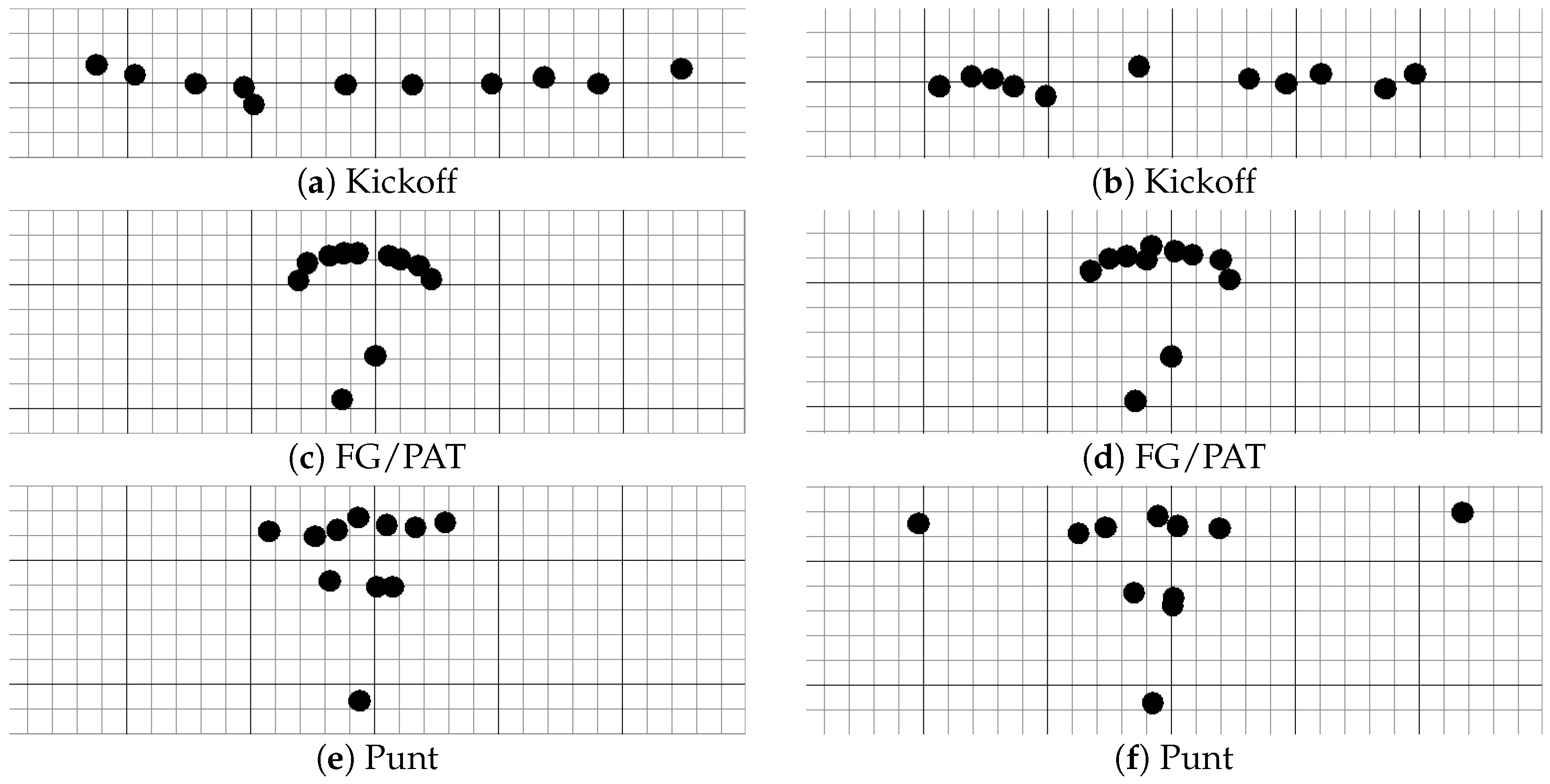
Electronics 13 03628 g003
Figure 4. Two examples of each special team play type present in the real-world dataset. Each black dot represents one player’s location in the x- and y-coordinates. (a,b) Kickoff, (c,d) FG/PAT, and (e,f) Punt.
Electronics 13 03628 g004
Figure 5. Two examples of real offensive play formations with the zones of each player position type transposed on top. Our data augmentation was achieved by randomly placing players into these zones depending on their position type according to the requirements outlined in Section 3.1.
Electronics 13 03628 g005
Figure 6. (a) A play formation from the Completed Dataset with colored zones indicating the possible range of variation of each player. (b) An example of the same formation after augmentation.
Electronics 13 03628 g006
Figure 7. (a) A play formation from the Completed Dataset with colored zones indicating the possible range of variation of each player. (b) An example of the same formation after augmentation with one player (right tackle) removed.
Electronics 13 03628 g007
Figure 8. Architecture of the MLP network. Between the input and output layers are two hidden layers with ReLU activations.
Electronics 13 03628 g008
Figure 9. The architecture of the play type recognition network, which takes in the x- and y-coordinates of the players to recognize the play type.
Electronics 13 03628 g009
Figure 10. The architecture of the player position recognition network, which takes in the x- and y-coordinates of the players and determines the position (role) of each player.
Electronics 13 03628 g010
Figure 11. Confusion matrix of the player position recognition accuracy when trained on the synthetic data and tested on the Original Dataset.
Electronics 13 03628 g011
Figure 12. Three example offensive play formations from the test dataset containing difficult-to-recognize wide receivers.
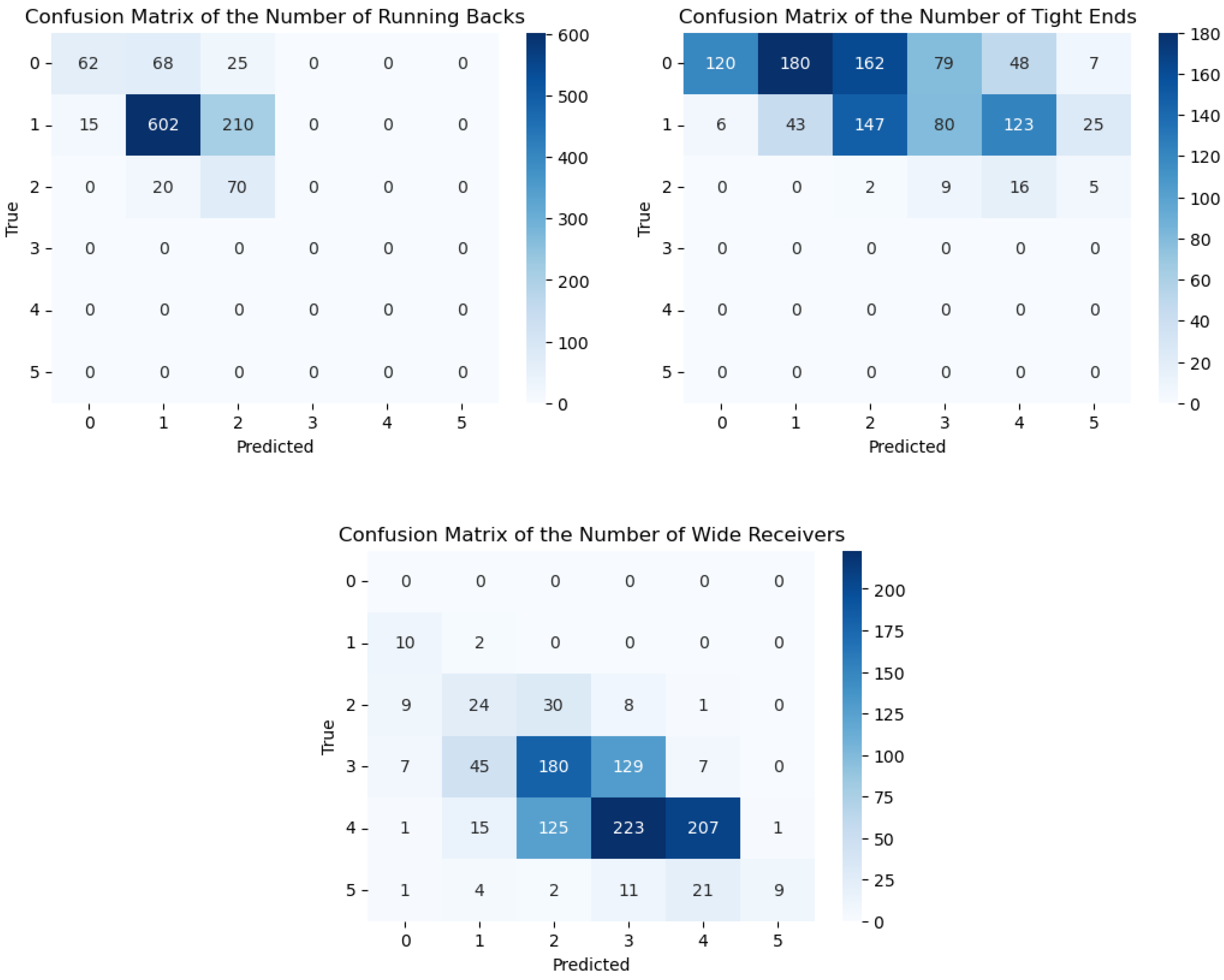
Electronics 13 03628 g012
Figure 13. Confusion matrices for the predicted number of running backs, tight ends, and wide receivers when trained with the Synthetic Dataset and tested on the Original Dataset.
Electronics 13 03628 g013
Figure 14. Confusion matrix of the play type recognition accuracy, when trained on the augmented 75% of the Completed Data, with the players shifted and tested on the 25% of the remaining Completed Dataset.
Electronics 13 03628 g014
Figure 15. Confusion matrix of the player position recognition model trained on the augmented 75% of the Completed Data with the player locations shifted. It was evaluated on the remaining 25% of the Completed Dataset.
Electronics 13 03628 g015
Figure 16. Confusion matrices for the predicted number of running backs, tight ends, and wide receivers with the model when trained on the augmented 75% of the Completed Data with the players shifted and tested on the remaining 25% of the Completed Dataset.
Electronics 13 03628 g016
Figure 17. Confusion matrix of the play type recognition accuracy when trained on the augmented 75% of the Completed Data with players shifted and up to two players removed and tested on the 25% of the Original Dataset that were not used to create the Completed Dataset.
Electronics 13 03628 g017
Figure 18. Confusion matrix of the player position recognition accuracy when trained on the augmented 75% of the Completed Dataset with players shifted and up to two players removed and tested on the 25% of the Original Dataset that were not used to create the Completed Dataset.
Electronics 13 03628 g018
Figure 19. Confusion matrices for the predicted number of running backs, tight ends, and wide receivers when trained on the augmented 75% of the Completed Dataset with players shifted and up to two players removed and tested on the 25% of the Original Dataset that were not used to create the Completed Dataset.
Electronics 13 03628 g019
Figure 20. Camera view angle from 45 degrees and 75 degrees above the football field and the bird’s-eye view captured from Madden 2020 video game.
Electronics 13 03628 g020
Table 1. Training and testing data and whether Play Type or Player Position Recognition was performed for each of the three tests.
TestTraining DataTest DataPlayPosition
120,000 Synthetic Data100% Original DataNoYes
275% Augmented Completed Data25% Completed DataYesYes
375% Augmented Completed Data25% Original DataYesYes
Table 2. Player position recognition accuracies when trained on the synthetic data and tested on the Original Dataset.
Player PositionRecognition Accuracy
Missing99.86%
Offensive Lineman84.33%
Quarterback/Running Back95.71%
Tight End25.15%
Left Wide Receiver79.76%
Right Wide Receiver68.53%
Table 3. Play Type recognition accuracies, when trained on the augmented 75% of the Completed Data with the players, shifted and tested on the 25% of the remaining Completed Dataset.
Play TypeRecognition Accuracy
Offensive Play98.42%
Kickoff98.80%
FG/PAT100.00%
Punt98.31%
Table 4. Player position recognition accuracies when trained on the augmented 75% of the Completed Data with the players shifted and tested on the 25% of the remaining Completed Dataset.
PositionRecognition Accuracy
Missing81.82%
Offensive Linemen98.92%
Quarterback/Running Back94.33%
Tight End0.38%
Left Wide Receiver95.55%
Right Wide Receiver94.68%
Table 5. Play type recognition accuracies when trained on the augmented 75% of the Completed Data with players shifted and up to two players removed and tested on the 25% of the Original Dataset that were not used to create the Completed Dataset.
Play TypeRecognition Accuracy
Offensive Play98.88%
Kickoff60.71%
FG/PAT100.00%
Punt88.71%
Table 6. Player position recognition accuracies when trained on the augmented 75% of the Completed Dataset with players shifted and up to two players removed and tested on the 25% of the Original Dataset that were not used to create the Completed Dataset.
Player PositionRecognition Accuracy
Missing96.94%
Offensive Linemen98.33%
Quarterback/Running Back94.25%
Tight End2.38%
Left Wide Receiver93.00%
Right Wide Receiver91.64%
Disclaimer/Publisher’s Note: The statements, opinions and data contained in all publications are solely those of the individual author(s) and contributor(s) and not of MDPI and/or the editor(s). MDPI and/or the editor(s) disclaim responsibility for any injury to people or property resulting from any ideas, methods, instructions or products referred to in the content.

