1. Introduction
Locating a stationary emitter from passive observations received by moving sensors is a problem that attracts much interest for both civil and defense-oriented applications in the signal-processing and underwater-acoustics literature, etc. Considering the relative motion between the emitter and the receiver, the Doppler effect is often used to estimate the position. The conventional methods usually estimate the intermediate parameters such as Frequency Difference of Arrival (FDOA) with respect to a reference receiver (also known as differential Doppler) [
1,
2], Doppler frequency shift [
3,
4] or Doppler Rate [
5,
6,
7], etc in the first step independently, and determine the position in the second step [
8,
9,
10]. However, these two-step methods are not guaranteed to yield optimal location results since they ignore the intrinsic constraint that all measurements should correspond to the same location [
11]. Avoiding the step of estimating the intermediate parameters, a novel localization conception known as Direct Position Determination (DPD) was presented [
12,
13,
14,
15,
16,
17,
18]. Emitter position is extracted directly through processing the raw signals in DPD. It has been proved that the localization accuracy of DPD is superior to the two-step method, especially at low signal-to-noise ratio (SNR) [
19,
20].
In the last decade, multiple Doppler effect based DPD algorithms have been presented. In [
21], Doppler frequency shifts based DPD was presented for narrow-band radio emitters which provides better accuracy than the two-step differential Doppler based method at low SNR no matter if the intercepted signals are known or unknown. By using a Minimum Variance Distortion Response (MVDR) estimator, the high resolution DPD of narrow-band signals based on FDOA is studied in [
22]. It can achieve higher resolution than the Maximum Likelihood (ML) type DPD since the MVDR is more sensitive to model errors in the steering vectors. In addition, some works also focus on the DPD of wide-band signals. Ref. [
23] advocates a DPD approach of wide-band emitters based on time delay and FDOA, and the closed-form expression for Cramer–Rao lower bound (CRLB) is also presented. Different with [
23], the received wide-band signals are partitioned into multiple non-overlapping short-time signal segments in [
24]. By coherent summation and non-coherent summation of the multiple short-time signal segments, novel DPDs were derived in it. The results show that both coherent summation-based and non-coherent summation-based DPD exhibit improved localization accuracy when the number of short-time signal segments increases. Considering that the previous DPD methods only exploit a single pulse, which is treated as an independent interaction even if the sensors received multiple pulses, Ref. [
25] proposed a multi-pulse coherent accumulation algorithm of DPD using the Time Difference of Arrival (TDOA) and FDOA for coherent short-pulse radar, which brings superior performance in accuracy and resolution.
Nevertheless, a multiple pulses accumulation will enlarge the observation window. Therefore, only using the Doppler frequency shifts cannot sufficiently reflect the Doppler effect since the Doppler frequency shift variation during each observation window is also noticeable. It is straightforward to infer that ignoring the Doppler frequency shift variations will result in a bias on the emitter location estimation in Doppler effect based DPD. Both the above inferences will be demonstrated in the simulations of this paper. To solve these problems, the Doppler rate, which is caused by relative acceleration, should be taken into consideration. Therefore, the utilization of Doppler rate in DPD is reasonable in two aspects. Firstly, it can enlarge observation window without the influence of the noticeable Doppler frequency shift variations. Secondly, it supplies additional information with respect to the emitter position which may result in a distinct increase in localization accuracy.
On the other hand, additional note should be set forth that these previous publications mainly focused on Doppler effect based DPD using multiple space separated sensors which has to synchronize and transfer data between different sensors. In this case, it is difficult to be implied in real applications especially for DPD which processes large amounts of raw signal data instead of the intermediate parameters in the two-step methods. To this end, DPD with a single moving receiver may be more practical.
Motivated by the above facts, this paper focuses on the Doppler and Doppler rate based DPD using a single moving sensor for coherent pulse trains. As studied in [
26], coherent pulse trains are portions of a continuous wave and the phases from pulse to pulse are in phase with the original wave. Without the measurement errors, all pulses may be generated from a single pulse by extrapolation. It is well known that coherent technologies are widely used in modern radar systems since their excellent performance in estimating range, radial velocity, and acceleration of a target. The relevant research can be found in [
27,
28,
29,
30]. With the aim to localize such an emitter, the proposed approach is derived and analyzed.
The main contributions of the work in this paper can be concluded as three aspects. Firstly, we take a first look at the problem of the noticeable Doppler frequency shift variation with a large observation window in Doppler effect based DPD and illustrate that it will result in a degradation of the localization accuracy in a Doppler frequency shift only based DPD. Secondly, we proposed a Doppler and Doppler rate based DPD approach to solve this problem which was not previously available. Finally, the theoretical lower bound (CRLB) for localization is also derived as a reference to examine the performance of the proposed method.
The rest of this paper is organised as follows.
Section 2 formulates the model of coherent pulse trains intercepted by a single moving sensor. In
Section 3, we derive the ML type DPD cost function.
Section 4 derives the CRLB, and
Section 5 provides the numerical simulations. The discussion and conclusions are made in
Section 6 and
Section 7, respectively.
2. Problem Formulation
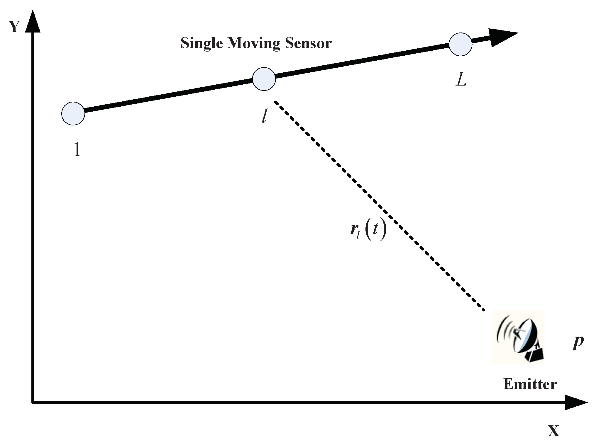
The formulation is in a 2D plane for ease of illustration. It is straightforward to extend to three dimensions. Consider a stationary emitter and a sensor with a single receiving antenna is moving relative to the emitter. The position of the emitter is denoted by the vector of coordinates
. The sensor intercepts coherent pulse trains of the emitter at
L interception intervals (also known as observation windows) along its trajectory. The starting velocity and acceleration of the sensor during the
l-th interception interval are denoted as
and
, respectively. The vector between the emitter and the sensor is
, and, therefore, in a interception interval
the distance between the sensor and the emitter
can be expanded by Taylor series as a second-order binomial
where
denotes the Euclidean norm of
,
where
stands for the initial position of the sensor during the
l-th interception interval,
is the radial velocity of the sensor at the start time of the
l-th interception interval and
is supposed to be the constant radial acceleration during the
l-th interception interval. Here, we do not further consider the higher order terms of
since generally they are quite small. Then, according to the principle of kinematics
where
stands for the transpose of
. In the second function of equation (
2), we take the scene where the sensor is maneuvering into consideration. If the receiver motion is supposed to be Recti Linear Constant Speed (RLCS), which is conventional in radar research, we just need to set
, resulting in
. It should be noted that the radial acceleration which will result in the Doppler rate can be produced even though the receiver is on a nonmaneuvering course. A possible localization scenario is presented in
Figure 1.
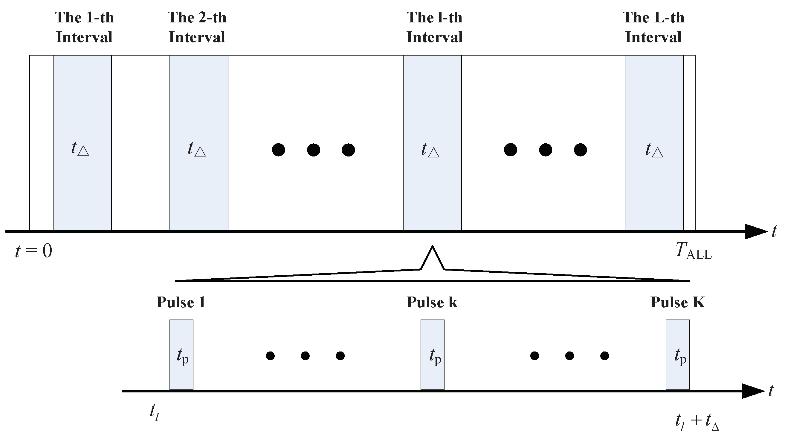
Hitherto, the relative motion relationship between the emitter and the sensor is established. Now, we formulate the model of the intercepted signals. At first, we define all the pulses during a single interception interval as a pulse train. Then, the emitted
L coherent pulse trains can be formulated as
where we suppose that each interception interval has
K pulses,
is the unknown envelope of the baseband transmitted signal of the coherent pulses as a function of the time
t, delayed by
, which is the transmitted time of the
k-th pulse from the emitter to the sensor during the
l-th interval.
is the nominal frequency of the transmitted signal, which is assumed to be known.
denotes the initial phase of the pulse trains, and
stands for a rectangular function which equals 1 at the interval
, where
is the pulse width.
To simplify the notations, consider each interception interval separately and replace
t with
where
is the start time of the
l-th interval,
is the length of the interception interval which is supposed to be the same for every interval. Meanwhile, hypothesize that no multipath exists in the system so that the intercepted noise-free pulse train during the
l-th interception interval appears as
where
is an unknown complex scalar representing the channel attenuation during the
l-th interval. Note that we do not assume any specific model for the relation between
and the location of the emitter, just suppose that
is fixed during the
l-th interval. In addition,
is the transmission delay where
c is the signal propagation velocity, and
. Note that
is the known time of arrival of the
k pulse during the
l-th interval relative to
where we further ignore the phase change of
caused by the Doppler effect which is very little due to the extremely short duration of pulses. To show the model of the signals in (
4) visibly, a schematic diagram is presented in
Figure 2 where
denotes the total observation time in it.
Define
where
is the Doppler frequency shift at the start time of the
l-th interception interval, and
denotes the Doppler rate which is approximately stationary during the
l-th interception interval. For the sake of simplicity, suppose that the receiver samples
N snapshots during each interception interval. Then, the received pulse trains of discrete signal model after being down converted to intermediate frequency can be formulated as
where
,
is the sampling period, and
. The intermediate frequency influenced by Doppler frequency shift
where
is the local frequency of the receiver, and
denotes the additive white Complex Gaussian noise.
Note that, in the previous research with respect to Doppler effect based DPD, is usually omitted since its small value compared with . However, with a large observation window , the Doppler frequency shift variation may be noticeable even if the receiver is on a nonmaneuvering course. In this paper, we take into consideration which can compensate this problem well.
To simplify the notations, we assume that every pulse has
M snapshots. Only consider the
k-th pulse during the
l-th interception interval, i.e., let
; then, (
6) can be formulated as
where the parameter
,
which spread over the pulse. Note that, for simplicity, we omit
in (
7) since
is much smaller than
. Next, we demonstrate it by an example. For a typical scenario,
Hz/s, assume that
coherent pulses with a constant pulse repetition interval (PRI)
ms are intercepted. Suppose the pulse width (PW) of the intercepted coherent pulse train
s and the sampling period
s, resulting in
. Then, we evaluate the terms
and
, and find that
. This result ends the proof.
To simplify the Formular (
7), define
with
where
denotes a diagonal matrix with
on the main diagonal; then, (
7) can be calculated as
It should be noted that the information with respect to the emitter position is embedded in
which includes the Doppler frequency shift
and the Doppler rate
, whereas the
of Doppler frequency shift only based DPD in [
21] omits the Doppler rate
.
Collecting the observations from all the interception intervals
Finally, the received coherent pulse trains are given by
To conclude, the problem at hand now is to use the measurements
given in (
11) to determine the position of the emitter
. To solve the problem of localization, the following assumptions are made:
The noise is temporally and spatially white and uncorrelated with the signals.
The coherent pulse trains have the same initial phase .
The envelope of the baseband from pulse to pulse is the same.
All of these assumptions are justified and frequently made in the related studies on the coherent pulse trains (see details in [
27,
28,
29,
30]).
5. Numerical Simulations
To show the effectiveness of the proposed method, we conduct the Monte Carlo simulations in this section. Note that the Doppler frequency shift variation can be produced even though there is no acceleration of the receiver. Its value depends on the length of the observation window and the related motion between the emitter and the receiver (see the model derived in (
2) and (
5)). With a large observation window, we illustrate the areas in which Doppler frequency shift variation is noticeable with different related motion in Example1 below. Meanwhile, considering the information of the emitter position is embedded in the Doppler frequency shift in DPD, Example 1 also reveals how the Doppler frequency shift variation affects the localization accuracy of the Doppler Frequency shift only based DPD, which is henceforth denoted by D-DPD. Note that [
25] has proposed a multiple pulse coherent accumulation based DPD using TDOA and FDOA with multiple moving sensors. As analyzed in it, coherent accumulation is mainly used to exploit the phase terms
during each interception interval, which is also involved in
in this paper. However, the TDOA between different sensors is nonexistent in the case of single moving sensor as considered in this paper. Thus, we carry out the D-DPD by following the approach in [
25] but omitting the TDOA and enlarging the observation window in it.
Subsequently, in Example 2, we examine the performance of the proposed DPD approach, which is henceforth denoted by DDR-DPD, and compare it with D-DPD, and CRLB.
Note that the localization root mean square error (RMSE) and bias are adopted as the criteria of localization accuracy, which are defined by
where
is the number of Monte Carlo trials and
is the estimated position at the
i-th trial. To obtain statistical results,
is set to be 250.
5.1. Example 1
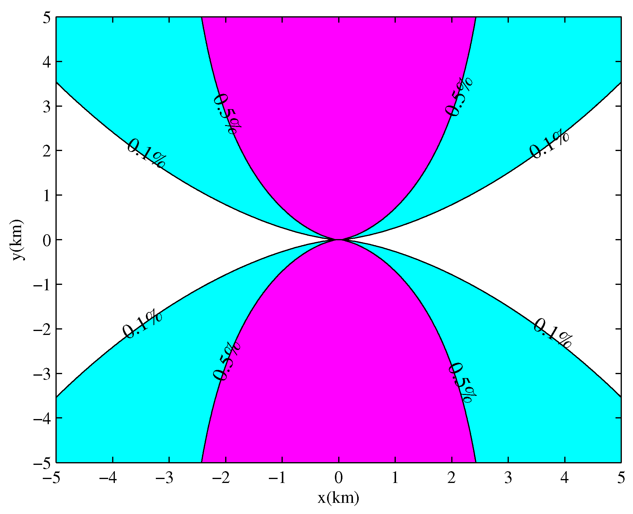
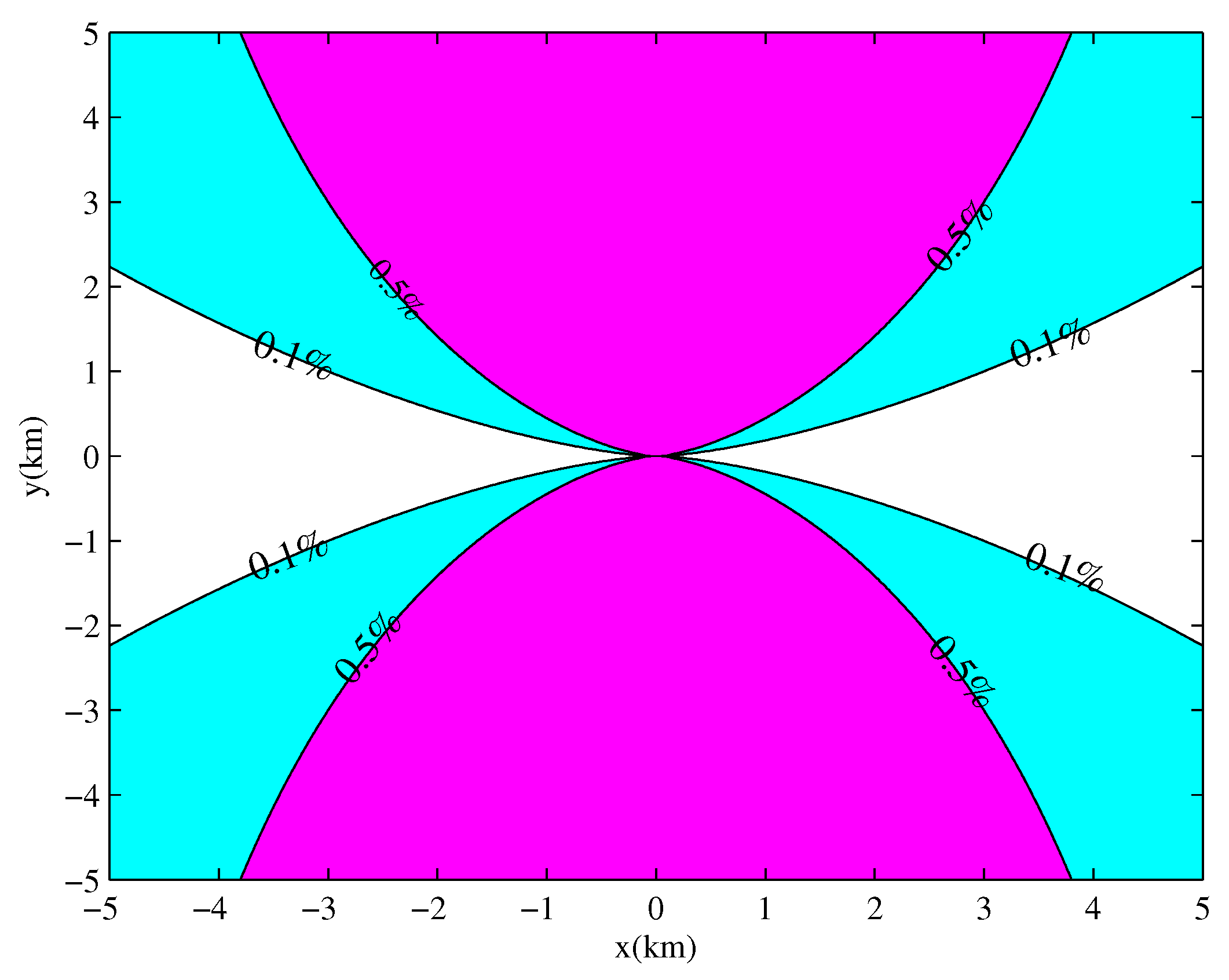
Assume that a stationary emitter locates at coordinate
km. The Doppler frequency shift will be produced if the signals are intercepted by a moving sensor. Define the Doppler frequency shift variation as
where
is the Doppler rate,
is the length of the observation window, and
is the initial Doppler frequency shift of the observation window.
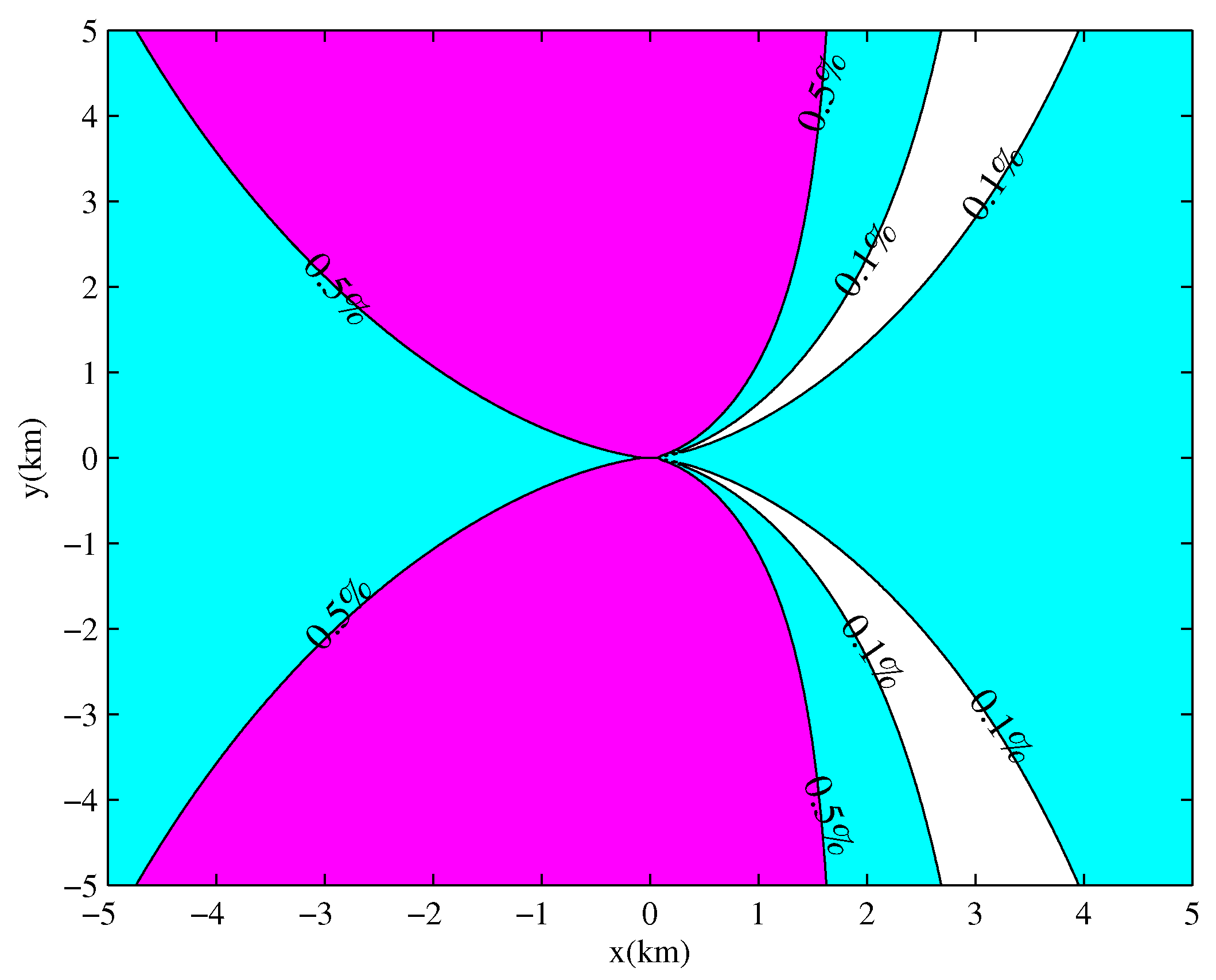
To evaluate the areas where
is noticeable, we assume that the receiver is moving in a space where
km and
km, and calculate
for each position of the receiver. Three motion types of the receiver are given in this simulation. Type 1 and type 2 are both RLCS but with different velocities which are
m/s and
m/s, respectively. Type 3 is the uniform acceleration motion with the velocity and the acceleration being
m/s and
m/s
, respectively. Set
ms (e.g., 200 coherent pulses of constant pulse repetition interval
ms are intercepted), the filled contour plots of the Doppler frequency shift variations are given in
Figure 3,
Figure 4 and
Figure 5.
We observe that the areas where the Doppler frequency shift variation is noticeable () is big enough so that it can not to be ignored especially when the receiver has a fast speed or an acceleration.
Next, we focus on how the Doppler frequency shift variation affects the localization accuracy of D-DPD. The layout of the system used during this simulation consists of a stationary emitter and a moving receiver which equips only a single receiving antenna. Concretely, the emitter locates at coordinate
km as described before, and transmits coherent pulse trains. The baseband transmitted signals of each pulse are unknown sinusoidal waves. The constant PRI is
ms, the pulse width (PW) is
us, the number of the intercepted pulses at each train is
K, and the initial phase
of the coherent pulse trains is selected at random from a uniform distribution over
for each Monte Carlo trial. The nominal frequency
GHz, and the signal received by the antenna is down converted to intermediate frequency
MHz. For simplicity, the sensor moves straightly from
km to
km. There are
interception intervals which start when the receiver is at coordinate
km,
km,
km,
km,
km, respectively. Three combinations of the initial velocity
and the constant acceleration
are displayed in
Table 1.
For Set Id , the receiver motion is supposed to be RLCS, and for Set Id , the receiver has a constant acceleration during all the interception intervals. Moreover, the channel attenuation is selected at random using normal distribution (mean = 1, std = 0.1), and the noise is complex white Gaussian whose amplitude is determined by the given . Note that the location determination is based on all the intercepted pulses with the sample frequency MHz.
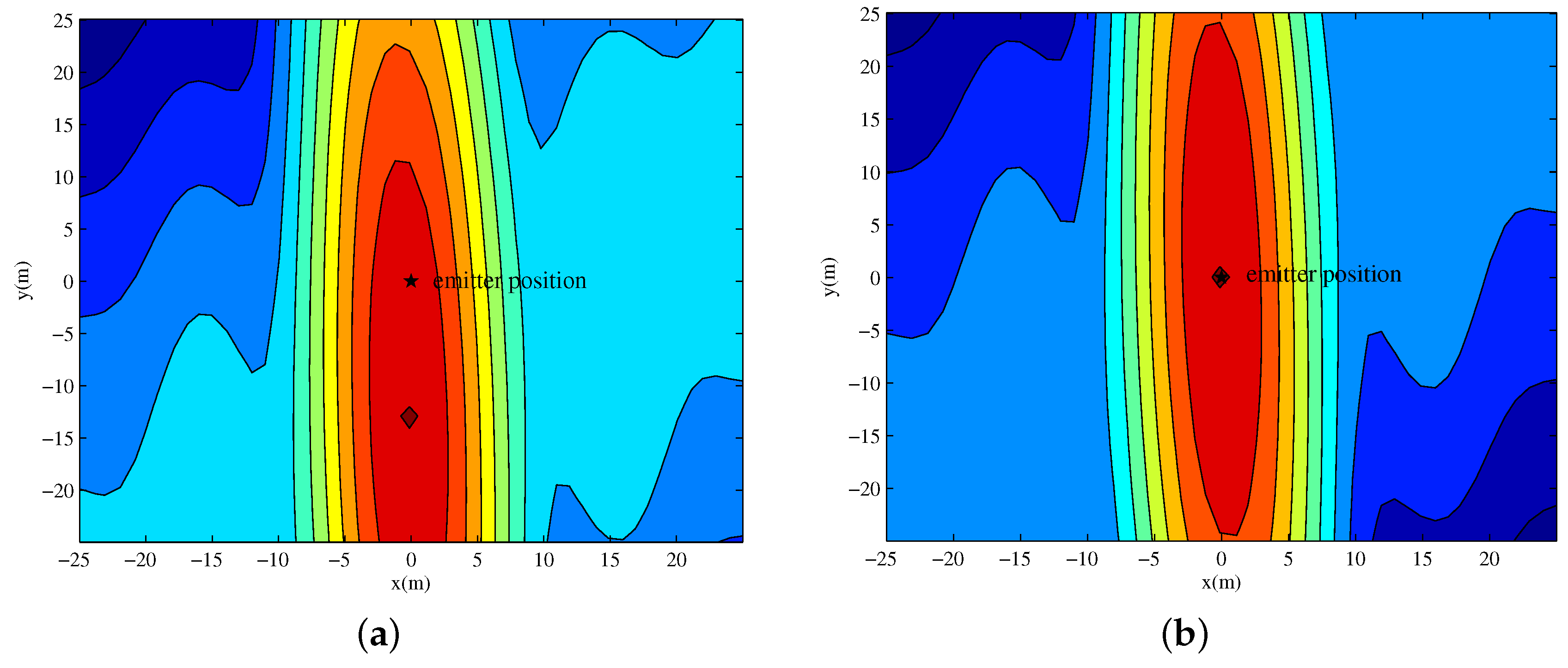
At first, set the number of pulses
K in each interception interval to be 200, resulting in
s. For the above scene with Set Id
, the noise-free spectrums of D-DPD and DDR-DPD are calculated by (
20). In order to display the peak of the spectrum clearly, the filled 2D contour plots of the spectrums are given in
Figure 6. As expected, the D-DPD has a positioning bias which is greater than 10 m, but the estimated position of the emitter in DDR-DPD coincides with its true position.
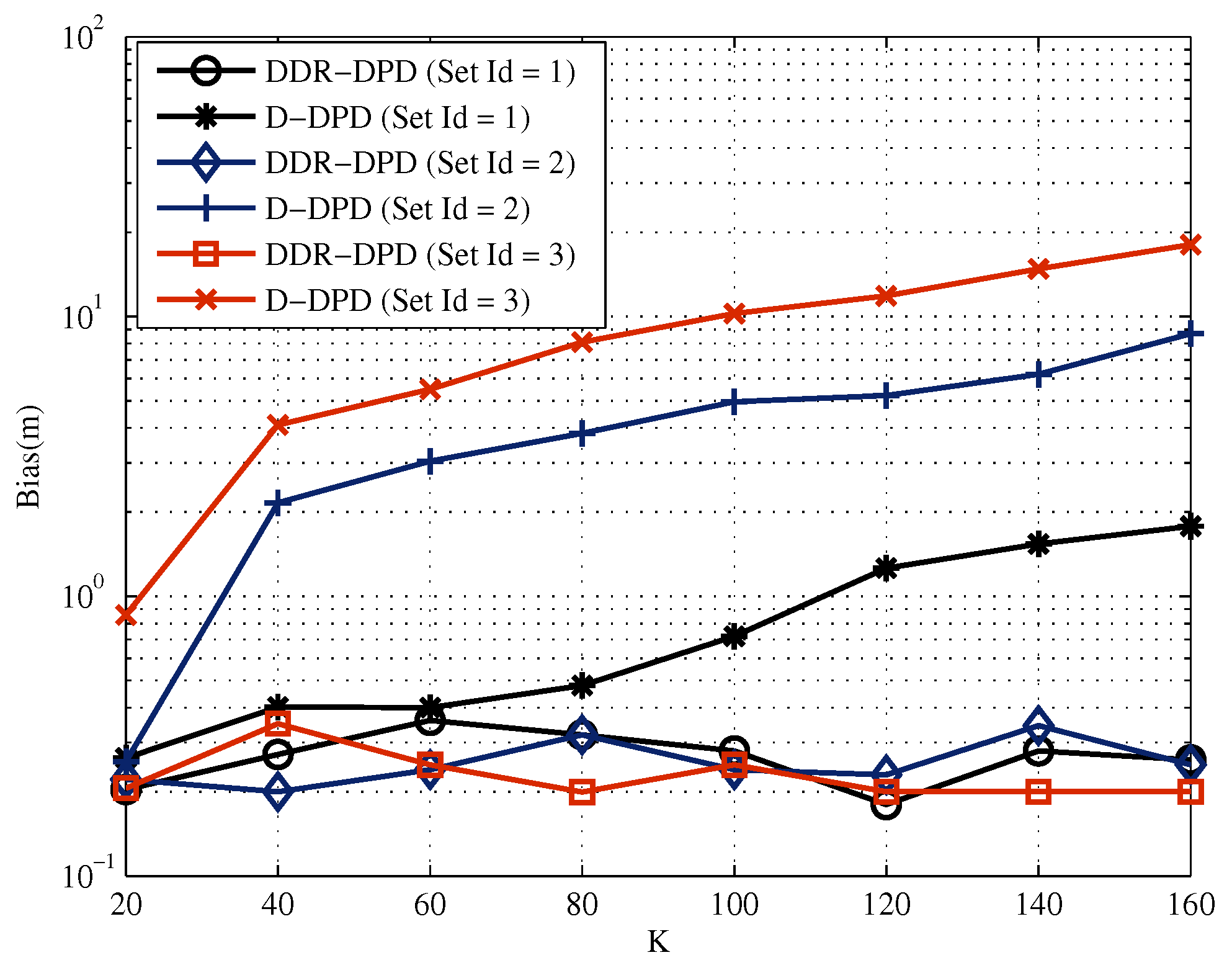
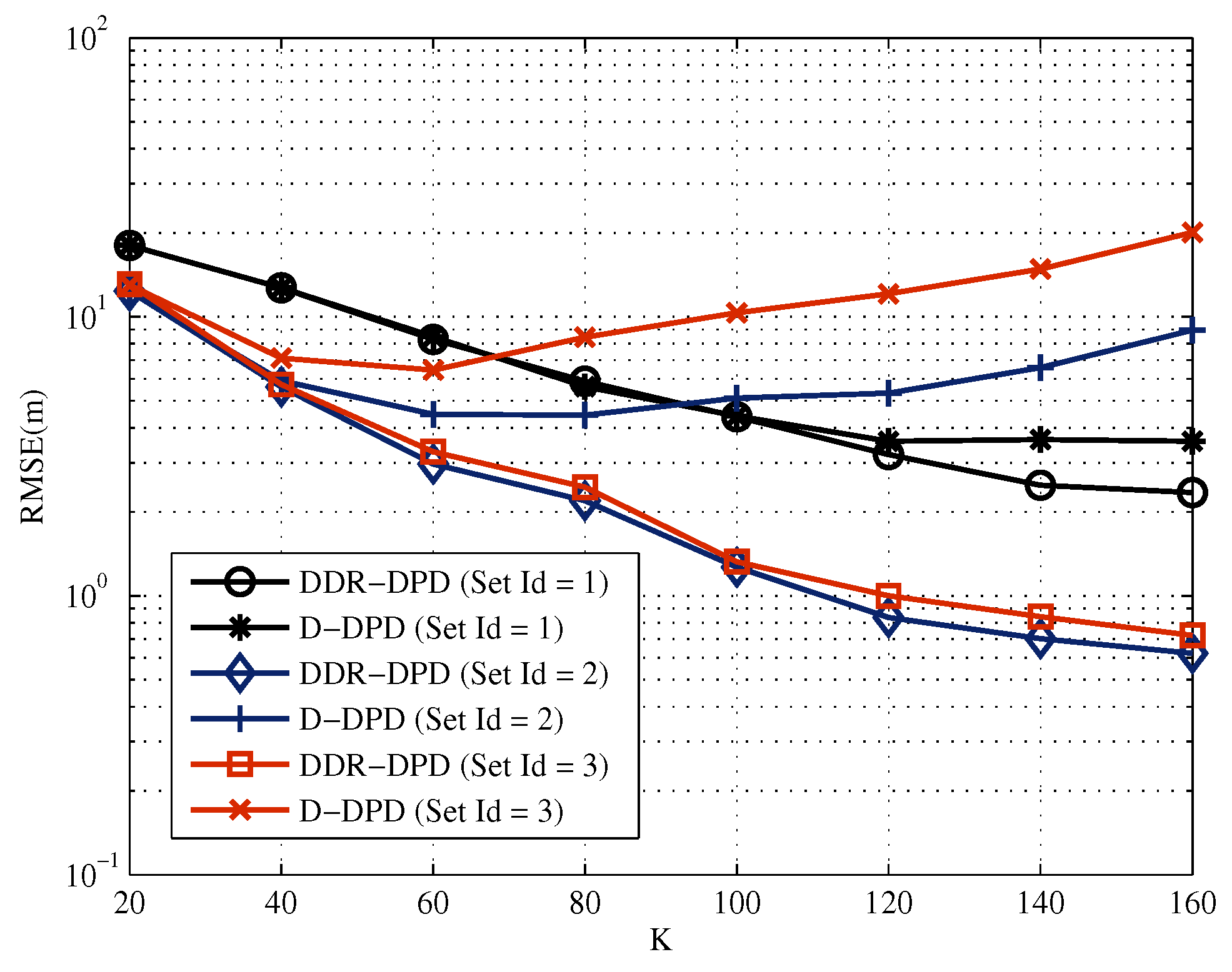
Afterwards, the bias and the RMSE are both calculated to analyze how the length of the observation window affects the localization accuracy. We fix the
dB, and vary the number of pulses
K in each interception interval from 20 to 160 to change the length of the observation window, which is given by
. Then, we illustrate the biases in
Figure 7 and the localization RMSE in
Figure 8. The results are both calculated with three motion types given in
Table 1. The bias and the localization RMSE of DDR-DPD are also plotted to be compared with D-DPD.
From
Figure 7 and
Figure 8, we observe that the biases of D-DPD increase with the increase of the pulse number
K of each interception interval, whereas the biases of DDR-DPD remain at small values. For Set Id
, the performance of DDR-DPD improves as the observation window enlarges since more effective information is involved. On the other hand, the performance of D-DPD declines as
K increases. For Set Id
, the two approaches yield similar localization performance when
. This is because the Doppler frequency shift variation is still small. In this case, the performance of D-DPD and DDR-DPD are both improved as the observation window enlarges since more pulses with respect to the emitter position are intercepted. However, the accuracy of D-DPD still declines when
, in contrast the performance of DDR-DPD improves. Note that there is a threshold of the observation window length
. When
, the localization accuracy of D-DPD will be significantly worse than DDR-DPD. For Set Id
, the
= 100 ms, 40 ms, 20 ms, respectively.
All the above results demonstrate that the performance of D-DPD and DDR-DPD will both improve as the observation window enlarges if the Doppler frequency shift variation is little. However, the Doppler frequency shift variation can not be ignored when large observation window and relative maneuvering course between emitter and receiver both exist. Large localization error will be produced if we omit the noticeable Doppler frequency shift variation.
5.2. Example 2
In this subsection, we take Set Id
for example and examine the performance of the proposed approach. First, set the pulse number
K of each coherent pulse train to be 100, and vary the
from
dB to 5 dB. The other parameters are the same with Example1. Calculate the RMSE of DDR-DPD and D-DPD, and the results are shown in
Figure 9a. In addition, the CRLB of localization using DDR-DPD derived in
Section 4 is also plotted which is denoted as CRLB in
Figure 9a.
We observe that the performance of DDR-DPD and D-DPD both improve as the SNR varied from
dB to 5 dB. However, the RMSE of DDR-DPD converges to the CRLB when
dB, and the RMSE of D-DPD approximately tends to be 5 m, which is exactly the bias of D-DPD as illustrated in
Figure 7. The underlying reason could be that the Doppler frequency variation is noticeable with the large observation window (
ms), which is omitted by D-DPD. As illustrated in Example 1, it will result in a bias that can not be eliminated by improving the SNR. On the other hand, the performance of DDR-DPD remains superior for all SNR (
dB) in this simulation. This is mainly caused by two reasons. At first, the bias which results from the noticeable Doppler frequency shift can be compensated in DDR-DPD but is involved in the RMSE of D-DPD. Secondly, the information with respect to the emitter position that is embedded in the Doppler rate is involved in DDR-DPD but is omitted in D-DPD.
Next, how the number of snapshots for each pulse affects the localization RMSE of the emitter is examined. We set the
dB, and the number of snapshots
M for each pulse varies from 200 to 1200.
Figure 9b shows the localization RMSE vs.
M. The localization CRLB of DDR-DPD is also plotted. We observe that the localization accuracy of DDR-DPD improves as
M increases. However, the performance of D-DPD is almost independent of the variation in
M. Moreover, the localization accuracy of DDR-DPD can reach the CRLB with moderate snapshots.
Note that, in this example, = 100 ms > = 40 ms. As expected in Example 1, the performance of DDR-DPD is superior to the performance of D-DPD. In addition, we observe that the superiority of the DDR-DPD will be more significant with the increase of the SNR and the number of snapshot M. Since RLCS model fits many kinds of real motions, it is justified to say that the proposed approach will have better applicability to the practical cases.
6. Discussion
We will discuss whether DDR-DPD has a good performance in practice from three aspects i.e., the necessity, the computation complexity and the possible implementation issues of the proposed method.
Firstly, as elaborated in the above sections, the proposed method shows superior performance in terms of localization accuracy compared with D-DPD when there is a noticeable Doppler frequency variation. In addition, the value of the Doppler frequency shift variation substantially depends on two factors i.e., the length of the observation window and the Doppler rate. To improve localization accuracy in DPD, multiple pulses accumulation can be used, which will unavoidably result in a large observation window (see
Figure 8). Meanwhile, we have known that the Doppler rate can be produced even if the receiver is in RLCS from (
2). In addition, the carrier frequency of the signals, its value depends on the position, the speed and the acceleration of the receiver and the emitter. Since the emitter is uncontrollable in a passive localization system, we can only decide the speed or the acceleration of the moving receiver. In a typical military or civilian scenario, the receiver can be equipped in an airplane or a satellite, etc. Generally speaking, the speed of the civil aircraft is between 150 m/s and 250 m/s, and the supersonic aircraft 340 m/s. The areas of the noticeable Doppler frequency shift variation with a speed similar to an aircraft have been illustrated in
Figure 3 and
Figure 4. It is justified to say that, with an unavoidably large observation window, the Doppler frequency shift variation is noticeable even the receiver is equipped in an aircraft, let alone a satellite that has much faster speed or even a conspicuous acceleration.
Secondly, the computation complexity of the proposed method is considered. The number of multiplications
required by the algorithm is imposed as an indicator of computation complexity. We compare DDR-DPD and D-DPD where exhaustive search are both used to estimate the emitter position. For the sake of simplicity, the small values e.g., the multiplications required by Eigenvalue Decomposition of a
matrix are ignored since it is independent from the number of the pulses and the snapshots. Then,
for DDR-DPD and
for D-DPD, where
stands for the number of the grid used in the exhaustive search and
D denotes the dimension of the considered scene. Generally speaking,
or 3, which is a small value, and the value of
L depends on the received signals which tends to be much larger than
D. In this sense, we fortunately observe that DDR-DPD does not introduce much more calculation than D-DPD as the computational complexities of them mainly both depend on the high order term
. However, the computational complexity may still be too high especially when there are multiple emitters because of the inherent flaw of ML but not the method itself. To relax the restrictions of the proposed method on practice, Alternating Projection [
15] can be utilized. Since the derivation is straightforward and not the main contribution of this paper, we will not present in-depth analysis of this problem.
Thirdly, we summarize two possible issues in terms of hardware based implementation of the proposed method i.e., the computation burden and the memory space. At first, the computation may be complex as discussed in the above paragraph. In addition, the DPD type approaches process the raw signals instead of the intermediate parameters as processed in the two-step method, which also increases the computational complexity. However, high-performance hardware equipment combined with a fast algorithm as also introduced in the above paragraph can deal with this problem very well. On the other hand, we also expect high demand for the memory space of the hardware as the proposed method needs to accumulate multiple interception intervals to estimate the emitter position. Nevertheless, large capacity FPGA are available easily now that can solve the problem straightway. In all of these three aspects, the proposed method may show a good performance in practice.
Moreover, inspired by [
24], the large interception window with multiple pulses can be partitioned into multiple short time segments. In this case, we may further hypothesize that each short time segment has a single pulse and each pulse has its individual Doppler frequency shift. This is also an interesting approach to substantially compensate the noticeable Doppler frequency shift variation which may exhibit similar performance compared with the proposed approach. However, this approach introduces
K unknown parameters in addition which will result in a complicated signal model and great computational complexity. We do not further provide a detailed study of this approach because it is beyond the scope of this paper. It may be an interesting topic for future investigations.
It also should be noted that DDR-DPD also maintains a superior performance for other general signals with a large observation window, although only the DDR-DPD of coherent pulse trains is considered in this paper. This is because the proposed model is more adapted to real situations when both a large observation window and relative acceleration between the emitter and the receiver exist.


