1. Introduction
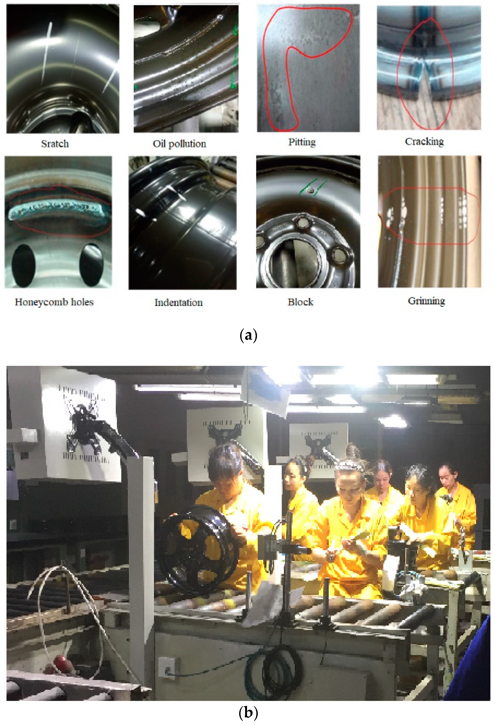
The automotive industry is an important part of the national economy, and the automobile is an essential means of transportation in daily life. The wheel hub is an important part of the automobile. In recent years, due to the rapid growth of production and imperfect processing technology, more than 40 kinds of defects in the hub are generated (see some examples in
Figure 1a). These defects will affect the good appearance of the product and brand image, and some defects will lead to serious traffic accidents. Therefore, the quality control is very important.
Due to the different definitions of hub defects at home and abroad, foreign testing equipment cannot meet the standards of the domestic enterprises, and hence many enterprises still employ manual inspection for complex surfaces. Nevertheless, the inter-class similarity and intra-class diversity of defects are the main difficulties for the detection. Traditional manual defect detection methods have great limitations, such as low efficiency and high labor costs. The most important problem of manual detection is its susceptibility to workers’ engagement degree and the level of relevant knowledge.
Machine vision detection provides the following advantages: High production efficiency, high automation level, good detection rate, and adaptability to the special industrial environment. Therefore, visual-based defect detection has been widely used in various fields, such as ceramic tile detection [
1], fabric detection [
2], and plant disease detection [
3]. Multiple studies have been performed on surface defect detection [
4,
5,
6,
7].
Gong at al. [
8] presented a method for the rapid detection of surface defect areas of strip steel. Five statistical projection features were extracted from the detection area of the surface image, and were used by the extreme learning machine (ELM) and region of background (ROB) pre-detection classifiers. A coating damage/corrosion detection device based on a three-layer feedforward artificial neural network was introduced by Reference [
9]. Krummenacher et al. [
10] designed an artificial neural network with constant cyclic movement to detect wheel deviation and roundness error, and they simulated the relationship between the inherent measurement values of these defects. Cha et al. [
11] used the deep convolutional neural network (CNN) to detect concrete cracks. The robustness and adaptability of their method were significantly improved compared with traditional edge detection methods (Canny and Sobel).
However, most methods can only detect specific types of defects, but cannot achieve accurate detection of multiple defects. Similarities between classes and the diversity within classes of defects make vision inspection challenging. At present, for complex workpieces with multi-curved surfaces, manual repeated inspection is commonly used in order to improve the detection rate. According to Cong et al. [
12], 57% of the enterprises follow similar procedures, and therefore intelligent and robust detection methods are urgently needed to replace manual detection.
These show the application value of this study. The fundamental reason why this application cannot be realized is the technical difficulty of generalization recognition using deep learning, such as the method of quickly generating the region proposal, the identification robustness of complex objects, and the balance between accuracy and time consuming, which are all aspects of the scientific value of this paper.
In this paper, a faster R-CNN method was developed to detect several common types of defects in fabricated wheel hubs. The developed method was arduously tested and compared to commonly used methodologies. The structure of this paper is as follows: Various solutions to defect or damages recognition are described in
Section 2. The generation of the image database for the wheel hub defects is described in
Section 3. The Faster R-CNN model and modified Faster R-CNN for multi-class defects of the wheel hub are explained in
Section 4. In
Section 5, the experimental procedure is depicted, the results of training, validation, and testing are discussed, and a comparison of the improved method with the state-of-the-art methods is presented.
Section 6 summarizes this research and future efforts.
2. Related Work
At present, several non-contact detection methods based on the traditional computer vision have been successfully applied. For example, an improved hub defect peak localization algorithm was proposed by Li et al. [
13]. They used a trend peak algorithm to extract the hub defect area and then a BP neural network to classify and identify the hub defect. In order to complete surface defect detection of printed circuit boards (PCBs), an effective similarity measurement method has been proposed [
14]. This method uses the adjoint matrix of two comparative images to calculate the symmetric matrix. The rank of the symmetric matrix is used as the similarity index of defect detection. The rank value of a defect-free image is zero, and the rank value of a defect image is obviously larger. However, this method cannot be adapted to multi-curved surface hub defect detection. A method based on hybrid chromosome genetic algorithms was conducted to classify metal surface defects [
15]. Similarly, aiming at metal surface defects, a method based on digital image singular value decomposition was developed by [
16]. Although these methods have improved somewhat, they still need some preprocessing and postprocessing techniques, and hence they are time-consuming. Additionally, the types of defects that they can detect are limited.
In order to solve the problems of image processing technology mentioned above, deep learning has been used. Deep learning combines low-level features to form more abstract high-level attribute representation and to discover distributed feature representation of data. Therefore, its excellent performance has been gradually employed by researchers since 2006. For example, Yi et al. [
17] adopted the end-to-end method based on a convolutional neural network to realize the identification and classification of seven defects of a particular steel product. A region-based convolutional neural network method has been adopted to detect ships [
18]. Aiming at the surface detection of solar panels with uneven structure and complex background, a visual defect detection method based on multi-spectral deep convolutional neural network (CNN) was designed by adjusting the depth and width of the network [
19]. A method based on a deep convolution neural network (DCNNS) for defect detection of parts and components was proposed by Reference [
20]. This method combines three serial detection stages based on DCNN and includes two detectors to locate the cantilever joint and its fasteners in turn, and incorporates a classifier to diagnose the fastener defects. Although all these methods can use sliding windows to locate defects, it is difficult to determine the size of sliding windows due to the different scales of defects in the test set.
Breakthroughs in object detection methods have always been driven by the success of regional proposed methods. For example, Girshick [
21] proposed a scale adjustable detection algorithm based on the combination of regional proposals and CNN in order to achieve multi-objective detection. This method had two key points: First, the convolution of the high-performance network was adopted to realize the bottom-up regional proposal localizing and segmenting the defects; second, pre-training supervision was conducted when training data was insufficient, and fine-tuning of the specified region was carried out to significantly improve performance. Compared with traditional CNN method with sliding windows, region-CNN (R-CNN) [
22] can significantly improve the accuracy of target detection. However, the method is time-consuming because it is not an end-to-end network, but three processes (CNN, regression, SVM) at the same time. Failure to implement computation sharing is a major cause of time consumption.
Time consumed in object proposal is the major bottleneck for detection technology. Aiming at this problem, Ross Girshick [
23] proposed the FAST R-CNN for object detection by training deep learning network VGG19. The operational speed of this method was nine times faster than that of R-CNN, and three times faster than that of SPP net. Moreover, it achieved the highest average precision (66%) and a detection time of 300 ms per image for PASCAL VOC 2012. However, the detection speed and precision of FAST R-CNN can be improved. Time-consuming and deficient training is generated, because the object proposal is implemented using external methods, such as selective search. To solve this problem, Ren et al. [
24] achieved a detection accuracy of 73.2% by combining region proposal network (RPN) and Fast R-CNN as one network through sharing features. The detection time of a single image was only 198 ms. This methodology greatly reduced the calculation cost and improved the detection accuracy by better training of the data. Several detection techniques have implemented the combination of RPN and Fast R-CNN. For example, Liu et al. [
25] used this combination in order to effectively detect the defects of complex texture fabrics. They adopted the non-maximum suppression and data enhancement strategies to improve the detection accuracy.
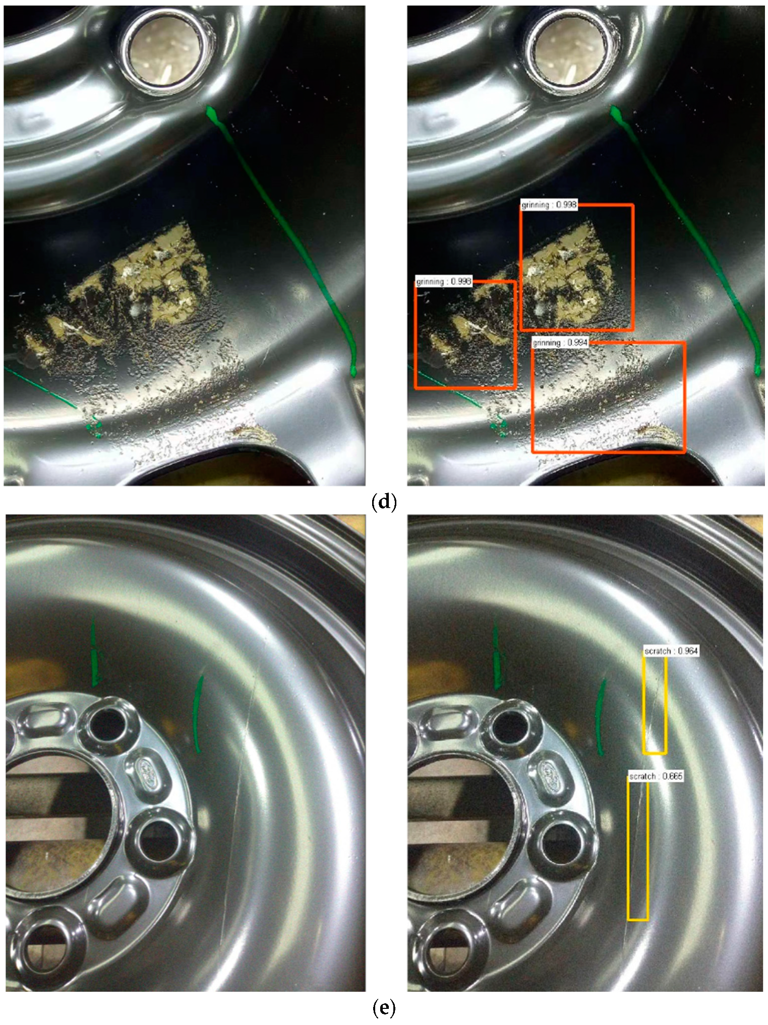
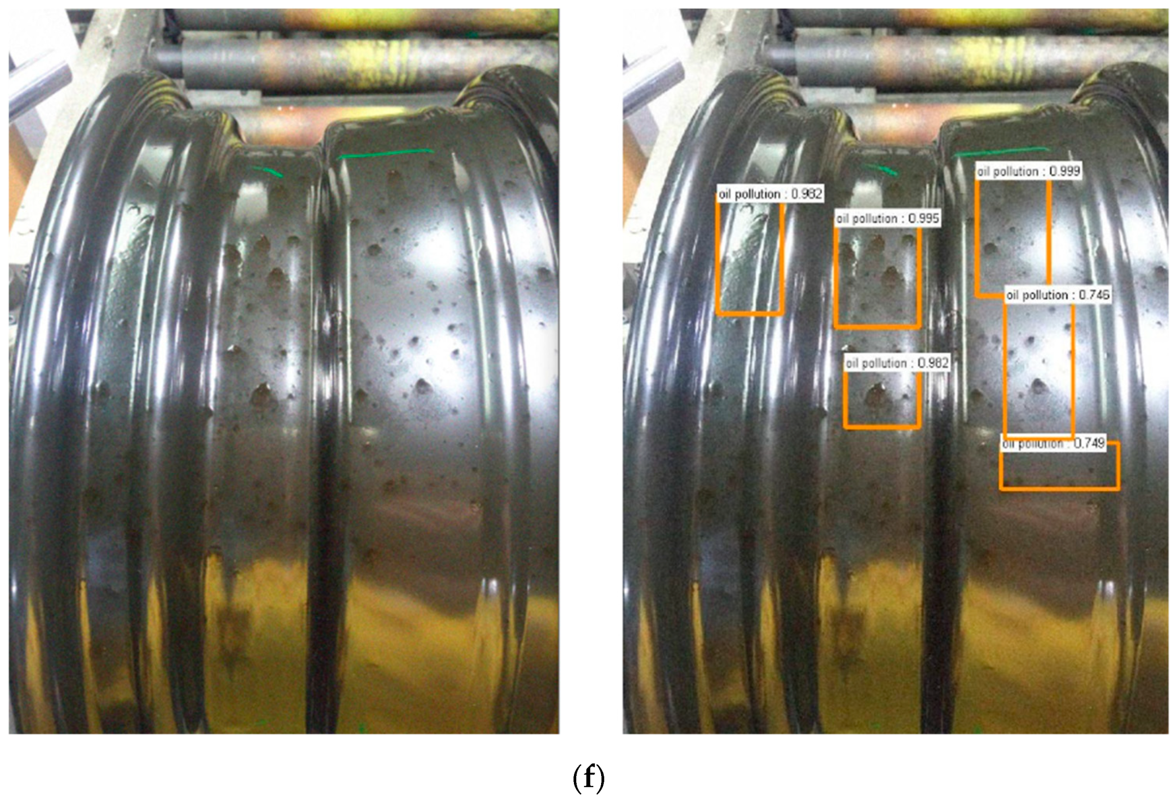
Inspired by the previous researches mentioned above, a new method was proposed by this research work to detect multi-class defects in wheel hubs. A faster R-CNN framework was modified to complete training, validation, and testing. Four defects (scratch, oil pollution, block and grinning,) of a wheel hub were used as representatives to achieve recognition and classification. More importantly, this flexible method can allow the easy addition of other defect types to the dataset in order to achieve universality.
4. Methods
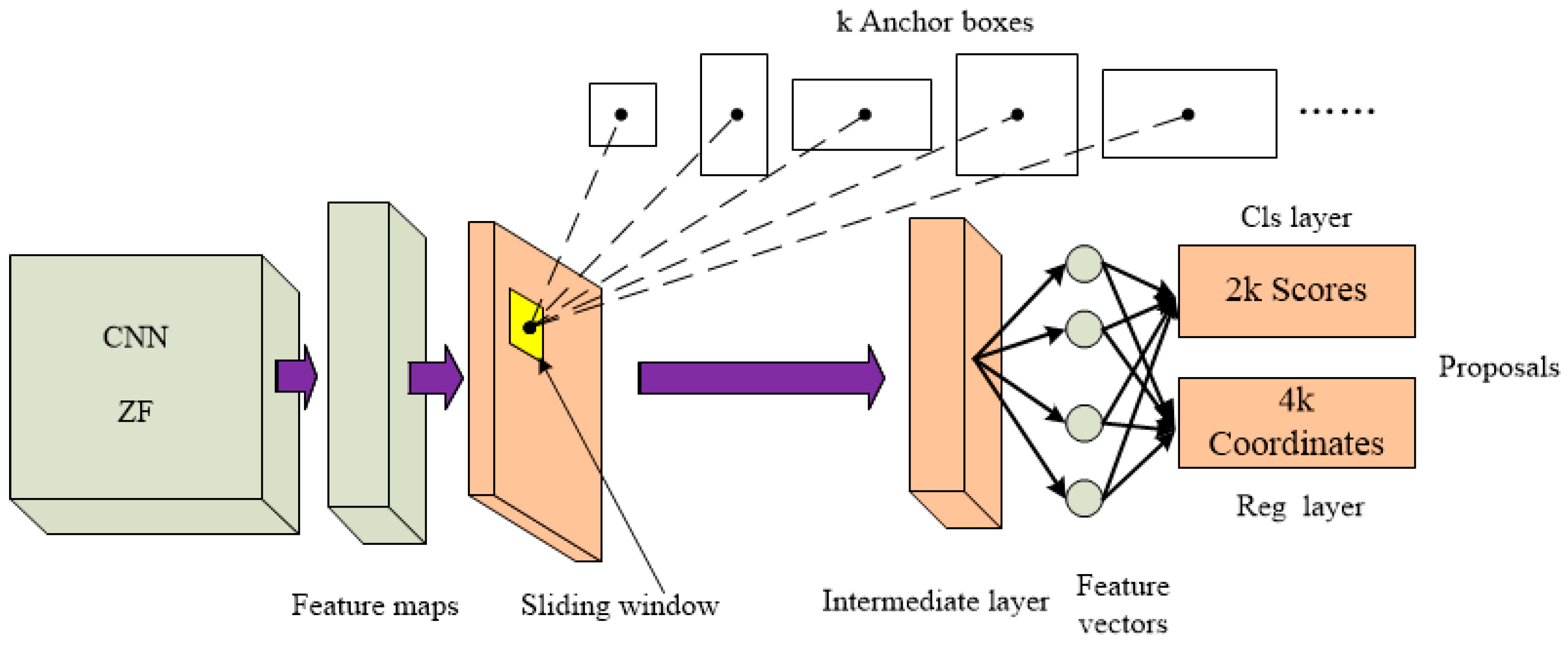
Faster R-CNN has been applied very well in the field of multi-target detection [
26], because RPN networks can generate object proposals with a high recall rate. As shown in
Figure 5, the original Faster R-CNN is composed of two networks. RPN and FAST R-CNN share the same convolution results. RPN is used to generate the proposals, and FAST R-CNN is used to accurately locate the object [
27]. However, due to the small number of available training samples with labels, the weight of the model cannot be initialized randomly, otherwise, it will easily lead to overfitting or non-convergence of the algorithm. Fortunately, transfer learning [
28] is a good way to solve this kind of problem. Accordingly, the mature classification model was adopted, and then the network structure was adjusted according to the specific object.
4.1. Regional Proposal Network (RPN)
The role of RPN [
24] is to generate proposals, including a rectangular box for proposals and probability of each proposal. The implementation of RPN is adopting a sliding window of n * n (in the paper, chose n = 3) to the convolution feature map of convolution layer 5–3, (conv 5–3) (in the paper, chose n = 3), then a length of 256 (Zeilerand Fergusmodel, ZF) [
29] or 512 (the Simonyan and Zisserman model, VGG16) [
30] fully connected network is generated. Two fully connected layers of the same level regression layer (reg layer), classification layer (cls layer) [
24] are following the 256-dimensional or 512-dimensional features. The reg layer is used to predict center coordinates and wide high value of the anchor, and the cls layer can be used to judge whether the proposal is an object or background as shown in
Figure 5. Sliding window ensures that the two layers are related to all the feature spaces of conv 5-3. In the RPN network, we need to focus on understanding the conception of anchors and loss functions.
4.1.1. Anchors
Multiple regional proposals are predicted simultaneously during the process of window sliding. For the proposals, there are k possible shapes of the prediction box, therefore the cls layer has 2k outputs (0/1), and the reg layer has 4k outputs (
,
,
,
). The k proposals for the same localization are called anchors. Anchor point is located in the center of the sliding window and related to the scale and aspect ratio. By default, we use 3 scales and 3 aspect ratios to generate
k = 9 anchors. So, for a convolutional feature map of size
(about 2400),
anchors are produced. The method of producing anchor with k-mean methods does not have translation invariance [
31], on the contrary, the anchor generated by this method has translation invariance. It is worth mentioning that translational invariance also reduces the model size, and then the number of parameters in the output layer is two orders of magnitude less than that in the multi- box method. Even considering the feature prediction layer, our method is still one order of magnitude less than the multi-box approach, which reduces the risk of overfitting on small data sets.
4.1.2. Loss Function
For training RPN, a binary class tag (object or no object) is assigned to each anchor point. To classify an anchor content as an object or no object, the following rules should be applied:
(1) The anchor point with the highest intersection over union (IoU) should be defined as a positive sample (see
Figure 6 and Equation (1)).
(2) The IoU with any truth box over 0.7 should be defined as positive samples.
(3) If the IoU between an anchor and any target area were less than 0.3, it should be judged as a negative sample.
Note that one ground-truth box can assign positive labels to multiple anchor points. Although the second condition is sufficient to determine the positive sample, the first rule is often used because sometimes the positive sample cannot be found in the second condition. Anchors that are neither positive nor negative contribute nothing to the training. With these definitions, an objective function is minimized after the multitasking loss of Fast R-CNN. The loss function of an image can be defined as [
24]:
where
is the serial number of the anchor points in each mini- batch,
and
are ground truth label (0/1) and the probability of anchor
being object,
and
are prediction box parameters and calibration box parameters, and
and
are classification loss function and regression loss function.
means that the regression is only applied to the positive sample (negative sample
). Cls-layer and reg-layer outputs are
and
.
The loss function was determined by normalizing (depend on mini batch size, here 256) and (depends on the number of anchor points, here 2400), and then weighting them by an equilibrium parameter (by default, ).
For the bounding box regression, the following four coordinates were parameterized:
,
,
, and
.
and
represent the central coordinates of a
×
box. Variables
,
, and
represent the prediction box, anchor box, and truth box, respectively. A similar convention is followed for derivate variables of
,
, and
. This can be considered as the anchor box regressing to the nearby ground truth box. The variables
and
in Equation (2) are used to define the geometrical differences between the predicted bounding box and anchor, as well as the ground truth box and the anchor. These geometrical differences are calculated as:
4.2. Faster R-CNN Model and Training
For the input of the region proposal in the Fast R-CNN [
32] network, a selective research method is adopted, which takes more time and limited optimization space for the whole system. However, Faster R-CNN used the RPN network to generate region proposal, which making efficiency jump again. Since Faster R-CNN is implemented by sharing the convolution layer of the RPN and the Fast R-CNN network, the RPN and Fast R-CNN cannot be trained independently, otherwise the parameters of the convolution layer will be changed. Therefore, training of the Faster R-CNN is more complex, and a four-step training strategy is adopted. The steps are as follows:
(1) The RPN network is trained separately, and the training model is initialized with ImageNet, and parameters are adjusted end to end.
(2) The detection network, Fast R-CNN, is trained independently. Object proposals for training are from RPN net in step 1, and the ImageNet model is adopted for model initialization.
(3) The parameters of step 2 are used to initialize the RPN model, but the convolution layer is fixed during the training, while the parameters belonging to the RPN in
Figure 5 are adjusted.
(4) Keep the shared convolutional layer fixed and use the RPN output proposals (step 3) as the input to fine-tune the parameters belonging to Fast R-CNN in
Figure 5.
4.3. The Improved Faster R-CNN
The ZF network [
29] and VGG [
30] are two commonly used networks in sharing convolution between RPN and Fast R-CNN. However, ZF net is known for its speed, which has been confirmed in the literature [
24,
33], and therefore this paper adopts the ZF net. In order to make the method adapt to multi-class defects detection for wheel hubs, we made the following improvements for ZF net. Firstly, we improved the original ZF net for the RPN. The last maximum pooling layer and full connection layer of ZF net were replaced by a sliding convolution layer, then a full connection layer with a depth of 256 was connected, and its softmax layer was replaced by a softmax layer and regression layer, which was
Figure 7.
Second, the ZF net was improved for the Fast R-CNN. The last maximum pooling layer was replaced by a region of interest (RoI) pooling layer. To prevent over-fitting during training, drop-out layers with a threshold of 0.5 were added in-between fully connected layers. The depth value of the final fully connection layers was changed to five (four types of defects and a background) to ensure compatibility. Finally, the softmax layer was replaced by the softmax layer and the regress regression layer (see
Figure 8).
As mentioned above, because the first nine layers of RPN and Fast R-CNN have the same structure in Faster R-CNN, CNN computing sharing was achieved.
Figure 9 shows the whole structure of the improved Faster R-CNN.
For one image, RPN may generate more than 2000 object proposals, which will lead to expensive calculation and may reduce the accuracy of detection. Therefore, the output of RPN was sorted according to the score of softmax layers. It is known that under the premise of not reducing the recognition accuracy, the number of proposals can be appropriately reduced to improve the detection speed. Accordingly, a maximum of 300 proposals was adopted by this investigation.
6. Conclusions
In the traditional CNN method, when a fixed sliding window is used to locate defects, it is difficult to determine the size of a window. Therefore, a method based on Faster R-CNN was proposed for detecting four kinds of defects (block, grinning, oil pollution, and scratches) on wheel hubs. Four hundred and two images (1440 × 1080 pixels) were collected. Data augmentation was accomplished by adding noise (Gaussian noise, gaussian blur, salt and pepper noise, and motion blur) to the original set of images. The resultant set of images was manually labeled. The training set, validation set, and testing set were generated by randomly selecting from these annotated images. In order to obtain the optimal detection accuracy, a trial and error method was adopted to set the initial parameters. In addition, the robustness of the network was verified by using 6 additional images. Furthermore, a comparative study was conducted with the popular methods R-CNN and YOLOv3.
For detecting and locating different kinds of defects, it is difficult to determine the advantages of each detection method because of the different training sets. However, it can be concluded that the structure of the proposed method based on network optimization has better computing efficiency, because RPNs can provide more flexible bounding boxes for different sizes of input images, and RPNs can efficiently and accurately generate regional proposals. Through sharing convolution features with downstream detection networks, the detection accuracy of the overall network can be improved.
Future detection methods based on this proposed method should improve the detection accuracy and robustness by using better quality images and wider shooting distances when building the image set. Finally, it is important to mention that Faster R-CNN can be certainly used to completely automate the detection of surface defects similar to those of the wheel hubs.


