Focusing of Ultrahigh Resolution Spaceborne Spotlight SAR on Curved Orbit

Abstract

Aiming to acquire ultrahigh resolution images, algorithms for spaceborne spotlight synthetic aperture radar (SAR) imaging typically confront challenges of curved orbit and azimuth spectral aliasing. In order to conquer these difficulties, a method is proposed in this paper to obtain ultrahigh resolution spaceborne SAR images on a curved orbit, which is composed of the modified RMA (Range Migration Algorithm) and the modified deramping-based approach. The modified RMA is developed to deal with the effect introduced by a curved orbit and the modified deramping-based approach is utilized to handle the problem of azimuth spectral aliasing. In the modified RMA, the polynomial expression of SAR two-dimensional spectrum on a curved orbit is derived with fourth-order azimuth phase history model and series reversion. Then, the singular value decomposition (SVD) is applied to decompose the expression of SAR two-dimensional spectrum numerically in order to acquire coordinates for Stolt interpolation in the scenario of curved orbit. In addition, the modified deramping-based approach is derived by introducing orbital state vectors in order to accommodate the situation of curved orbit in the proposed method. Experiments are implemented on point target simulation in order to verify the effectiveness of the presented method. In experiments, the range and azimuth resolution can achieve 0.15 m and 0.14 m, with focused scene size of 3 km by 3 km.

1. Introduction

Synthetic aperture radar (SAR) has become an indispensable means for remote sensing, which is competent to provide high resolution images and videos for monitoring various targets under any weather condition [1,2,3,4,5,6,7]. With the desire for higher resolution, the future task of spaceborne SAR challenges the development of SAR imaging algorithms [8]. However, traditional SAR imaging algorithms perform disappointedly with the requirement of ultrahigh resolution in a spaceborne scenario. Various influences occur when the resolution achieves decimeter level in low earth orbit (LEO) spaceborne SAR, which have responsibility for the unsatisfied focusing performance [9]. Curved orbit and azimuth spectral aliasing are two of these influences which remain to be solved.

Traditional SAR imaging algorithms are derived from an assumption that the radar platform has linear movement with constant velocity [10]. Nevertheless, this assumption is no longer accurate when spaceborne SAR is expected to achieve ultrahigh resolution at the decimeter level. Therefore, the difference between the theoretical assumption and real orbit degrades the imaging quality in the azimuth direction. Aiming to solve this problem, a sequence of algorithms have been developed in order to cope with spaceborne spotlight SAR on a curved orbit, which describe the relative satellite-earth motion using Taylor expansion with azimuth time [11,12,13,14]. In the literature [11], a slant range model based on fourth-order Taylor expansion is firstly proposed and is implemented to process spaceborne spotlight SAR data on a curved orbit. An advanced RMA (Range Migration Algorithm) is proposed in [12] for dealing with high resolution spaceborne spotlight SAR imaging. The RMA is also known as the ωK algorithm [15]. In [12], a slant range is derived according to the model in [11] so as to accommodate the curved orbit. Moreover, a method for achieving the analytical expression of two-dimensional (2D) point target spectrum for bistatic SAR is presented in [16] and is applied for bistatic SAR imaging in [17], which is obtained via associating the slant range model in [11] with series reversion [18]. Subsequently, a method, which is named as generalized ωK, is proposed by combining multivariable Taylor expansion with the derivation of 2D spectrum in [16]. The generalized ωK presented in [13] is utilized to deal with geosynchronous spotlight SAR on a curved orbit. Consequently, the generalized ωK is extended to adapt for SAR data with squint angle in [14]. Although, the algorithms presented in [13,14] perform satisfactorily in the case of geosynchronous spotlight SAR, the phase error induced by the first-order multivariable Taylor expansion cannot be neglected when resolution attains decimeter level. Apart from algorithms derived from the slant range model in [11], the singular value decomposition Stolt (SVDS) presented in [19] offers another approach for settling the problem caused by curved orbit. The SVDS associates the singular value decomposition (SVD) with ωK algorithm so as to deal with spaceborne spotlight SAR in the scenario of curved orbit.

In order to deal with ultrahigh resolution spaceborne spotlight SAR on a curved orbit, the modified RMA is proposed in this paper. The modified RMA is developed to handle the effect introduced by curved orbit in the scenario of spaceborne spotlight SAR. In the modified RMA, the 2D spectrum of echo data on a curved orbit is derived via the range model in [11] and series reversion. Then, the expression of 2D spectrum of reference point is utilized to perform reference function multiplication (RFM). After RFM operation, point at reference range has been fully focused, and a residual phase exists for targets at other ranges. Afterwards, SVD is utilized to numerically decompose the expression of 2D spectrum in order to acquire coordinates for Stolt interpolation. Subsequently, Stolt interpolation is implemented to perform the residual range cell migration correction, residual secondary range compression and residual azimuth compression. Then, focused image can be obtained via inverse 2D Fourier transform. Although the generalized ωK in [13] is capable of processing echo data on a curved orbit, the phase error caused by the first-order multivariable Taylor expansion seriously degrades image quality when resolution achieves 0.14 m. Meanwhile, the phase error induced by SVD is much smaller than the first-order multivariable Taylor expansion on numerical decomposition of 2D spectrum. As a result, the modified RMA performs better than the generalized ωK when resolution achieves 0.14 m in azimuth direction. The modified RMA is presented in this paper as a part of the proposed method.

In addition to curved orbit, azimuth spectral aliasing is another problem which stems from high azimuth resolution requirement under the circumstance of LEO. The deramping-based approach for solving azimuth spectral aliasing is firstly proposed in [20] and extended to squinted spotlight SAR imaging in [21]. However, deramping-based approaches in [20,21] are only discussed under the condition that the SAR platform moves uniformly in a linear track. Orbital state vectors, which are capable of estimating Doppler parameters in the scenario of curved orbit, are implemented to modify deramping-based approach in order to accommodate the curved orbit in this paper. As a consequence, a modified deramping-based approach is presented in this paper as a part of the proposed method.

The proposed method comprises of modified RMA and modified deramping-based approach. The traditional RMA and the traditional deramping-based approach is only capable of dealing with the scenario of uniform linear motion. The modified RMA extends the traditional RMA to the scenario of curved orbit and the modified deramping-based approach achieves the same purpose. In addition, the modified RMA is developed based on the generalized ωK and has much smaller phase error than the generalized ωK when azimuth resolution achieves 0.14 m. Consequently, the proposed method performs better than the generalized ωK when azimuth resolution achieves 0.14 m in the situation of LEO on a curved orbit.

The proposed method is the improvement on the generalized ωK in [13]. Although the generalized ωK performs well in the scenario of geosynchronous SAR on a curved orbit, it is unable to cope with ultrahigh resolution spaceborne spotlight SAR in the scenario of LEO on a curved orbit. The generalized ωK lacks means to solve the azimuth spectral aliasing problem when azimuth resolution is expected to achieve 0.14 m. Additionally, the phase error in the generalized ωK becomes unbearable under the ultrahigh resolution requirement. The modified deramping-based approach aims to cope with azimuth spectrum aliasing and the modified RMA has much less phase error when azimuth resolution is desired to achieve 0.14 m. Point target simulation is operated to confirm the validity of the proposed method under the circumstances of LEO. In simulation, the swath width of the illuminated scene achieves 3 km in range direction and 3 km in azimuth direction. Furthermore, resolution of focused targets can achieve 0.15 m and 0.14 m in range and azimuth direction, respectively. The proposed method is compared with the generalized ωK. Results in simulation show that the proposed method has smaller phase error and performs better than the generalized ωK. Vectors and matrices are in bold italic while variables are in italic in this paper. The rest of this paper is organized as follows. Section 2 describes the proposed method. Then traditional RMA is briefly presented. Then, the modified RMA and the modified deramping-based approach are derived and described in details. In addition, procedure of the proposed method is also illustrated in this section. Section 3 presents experimental results of simulation in order to validate the effectiveness of the proposed method. Discussion of experiments is drawn in Section 4. Finally, Section 5 gives the conclusion.

2. Methodology

2.1. Traditional RMA

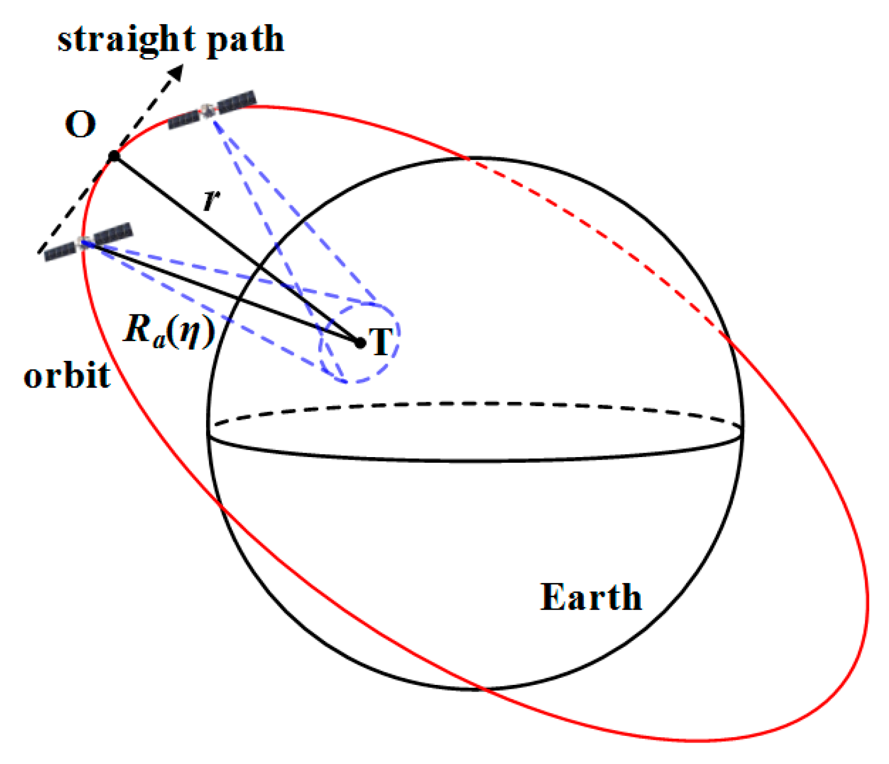
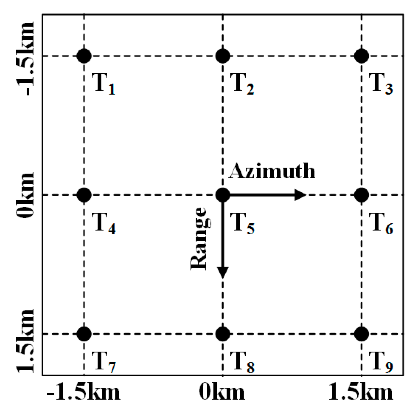
In this part, a brief introduction on traditional RMA is demonstrated. The geometry of spaceborne spotlight SAR is shown in Figure 1. The black dashed track with an arrow in Figure 1 denotes approximate straight path while the red ellipse represents curved orbit of true satellite motion. In Figure 1, the blue dashed lines and circle illustrate that the beam illuminates the target all the time during collecting SAR data. T denotes the illuminated target and O denotes the position of zero Doppler on the curved orbit. R_a(η) is the slant range between the radar and a target at azimuth time η and r represents the closest slant range.

The traditional RMA is acquired under the consideration of uniform linear motion. After modulation to baseband, the echo signal of point target T is able to be described in terms of range time τ and azimuth time η as follows:

$$\mathit{s}(\tau ,\eta ;\mathrm{T})={\mathit{w}}_{\mathit{r}}\left[\tau -\frac{2{\mathit{R}}_{\mathit{a}}(\eta )}{c}\right]{\mathit{w}}_{\mathit{a}}(\eta )\exp \left[\frac{-j4\pi f_0{\mathit{R}}_{\mathit{a}}(\eta )}{c}\right]\exp \left\{j\pi K_r{\left[\tau -\frac{2{\mathit{R}}_{\mathit{a}}(\eta )}{c}\right]}^2\right\}$$

(1)

The amplitude factors have been ignored. w_r(•) is the range envelope, w_a(•) is the azimuth envelope, c is the velocity of light, K_r is the range frequency modulation rate, f₀ is the carrier frequency and j is the imaginary unit.

In the scenario of uniform linear motion, the slant range is modelled by the hyperbolic equation with the velocity v and closest slant range r as follows:

$${\mathit{R}}_{\mathit{a}}(\eta )=\sqrt{r^2+v^2{\eta }^2}$$

(2)

By performing 2D Fourier transform (FT) on Equation (1) via the method of stationary phase with the slant range model in Equation (2), the 2D spectrum of echo signal can be represented as follows:

$${\mathit{S}}_{\mathbf{2}\mathit{df}}(f_{\tau },f_{\eta };\mathrm{T})={\mathit{W}}_{\mathit{r}}(f_{\tau }){\mathit{W}}_{\mathit{a}}(f_{\eta })\exp \left[-j\frac{4\pi r}{c}\sqrt{{\left(f_0+f_{\tau }\right)}^2-\frac{c^2{f}_{\eta }^2}{4v^2}}-j\pi \frac{f_{\tau }^2}{K_r}\right]$$

(3)

In Equation (3), f_τ and f_η are range and azimuth frequency, respectively. And W_r(•) is the envelope of the range frequency while W_a(•) is the envelope of the azimuth frequency.

The first step in traditional RMA is the RFM. The reference function in 2D frequency domain can be chosen as conj[S_2df(f_τ,f_η;T_ref)], which is the conjugated 2D spectrum of the reference target. T_ref denotes the reference point target and conj[•] denotes conjugation operation.

The RFM operation can be expressed as follows:

$$\begin{array}{ll}{\mathit{S}}_{\mathit{RFM}}(f_{\tau },f_{\eta };\mathrm{T})& ={\mathit{S}}_{\mathbf{2}\mathit{df}}(f_{\tau },f_{\eta };\mathrm{T})\mathrm{conj}\left[{\mathit{S}}_{\mathbf{2}\mathit{df}}(f_{\tau },f_{\eta };{\mathrm{T}}_{\mathrm{ref}})\right]\\ & ={\mathit{W}}_{\mathit{r}}(f_{\tau }){\mathit{W}}_{\mathit{a}}(f_{\eta })\exp \left[-j\frac{4\pi (r-r_{ref})}{c}\sqrt{{\left(f_0+f_{\tau }\right)}^2-\frac{c^2{f}_{\eta }^2}{4v^2}}\right]\end{array}$$

(4)

The RFM operation completely cancels the range migration of all targets at the reference range. Nevertheless, the RFM only partly corrects the range migration of targets at other ranges. Therefore, a subsequent Stolt interpolation is implemented so as to compensate the residual quadratic and higher order phase modulation. In the scenario of uniform linear motion, The Stolt interpolation is defined as follows:

$$\sqrt{{\left(f_0+f_{\tau }\right)}^2-\frac{c^2{f}_{\eta }^2}{4v^2}}=f_0+f_{\tau }^{\prime }$$

(5)

After implementation of Stolt interpolation, the SAR data is transformed into the new domain ($f_{\tau }^{\prime }$, f_η) as follows:

$$\begin{array}{l}{\mathit{S}}_{\mathit{RFM}}^{\prime }(f_{\tau }^{\prime },f_{\eta };\mathrm{T})\\ ={\mathit{W}}_{\mathit{r}}(f_{\tau }^{\prime }){\mathit{W}}_{\mathit{a}}(f_{\eta })\exp \left[-j\frac{4\pi (r-r_{ref})}{c}(f_0+f_{\tau }^{\prime })\right]\end{array}$$

(6)

By performing 2D Inverse FT to Equation (6), the echo data can be transformed into time domain. As a result, a finely focused SAR image is acquired as follows:

$${\mathit{I}}_{\mathit{RFM}}^{\prime }(\tau ,\eta ;\mathrm{T})=\sin \mathrm{c}\left[\tau -\frac{2(r-r_{ref})}{c}\right]\sin \mathrm{c}(\eta )$$

(7)

2.2. Modified RMA

When spaceborne spotlight SAR is desired to achieve ultrahigh resolution in decimeter level, the motion of platform of SAR is unable to be treated as uniform linear motion. Therefore, curved orbit is required to be considered in algorithms for SAR imaging. The modified RMA is proposed to deal with SAR data on curved orbit. In the modified RMA, the expression of 2D spectrum of echo data is derived by combining the range model in [11] with series reversion. Subsequently, the formula of 2D spectrum of reference point is used to implement RFM operation. Then, SVD is applied for numerically decomposing the expression of 2D spectrum so as to obtain coordinates for Stolt interpolation. After Stolt interpolation, focused image is able to be acquired via 2D inverse Fourier transform.

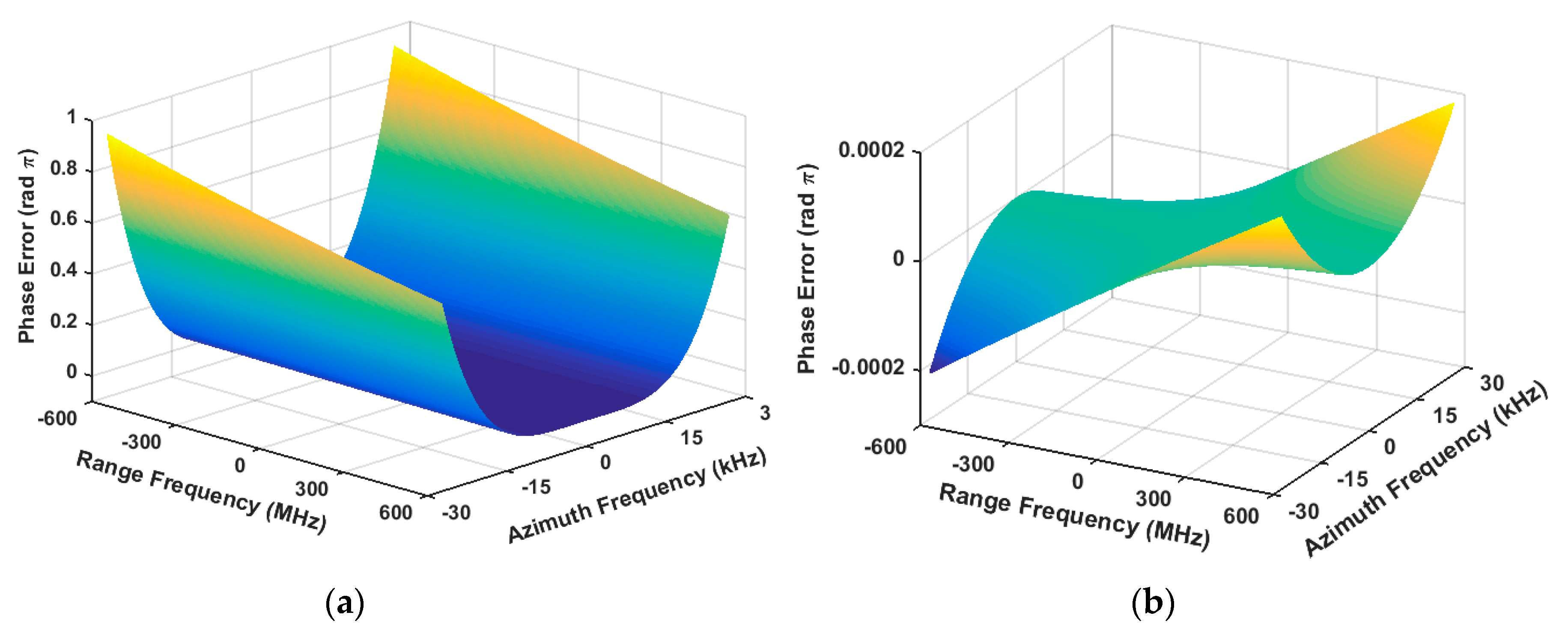
In comparison with the traditional RMA, the slant range model and the expression of the 2D spectrum in modified RMA are capable of accommodating the curved orbit while the traditional RMA is only able to deal with the scenario of uniform linear motion. Additionally, although the generalized ωK is able to cope with the scenario of curved orbit, the modified RMA has much smaller phase error than the generalized ωK when azimuth bandwidth is larger than 49 kHz. SVD, which is applied in modified RMA, is able to provide numerical decomposition with much smaller phase error than the first-order multivariable Taylor expansion in the generalized ωK. Therefore, the modified RMA performs better than the generalized ωK when the azimuth resolution achieves 0.14 m. The modified RMA is derived and presented in this part.

In the scenario of curved orbit, the slant range is inaccurate to be modelled as the hyperbolic equation in Equation (2). Therefore, it is necessary to utilize more accurate slant range model for curved orbit. The slant range model in the literature [11] is capable of modelling the slant range between radar and target in the scenario of curved orbit. According to the literature [11], the slant range between the radar and a target can be expressed in terms of azimuth time η as follows:

$${\mathit{R}}_{\mathit{a}}(\eta )=\sqrt{e_0+e_1\eta +e_2{\eta }^2+e_3{\eta }^3+e_4{\eta }^4}$$

(8)

The definitions of e₀, e₁, e₂, e₃ and e₄ are presented from Equations (9)–(13). And ◦ denotes inner product operation.

$$e_0=\mathit{R}\circ \mathit{R}$$

(9)

$$e_1=2\mathit{V}\circ \mathit{R}$$

(10)

$$e_2=\mathit{A}\circ \mathit{R}+\mathit{V}\circ \mathit{V}$$

(11)

$$e_3=\mathit{A}\circ \mathit{V}+\frac{1}{3}\left(\mathit{R}\circ \mathit{B}\right)$$

(12)

$$e_4=\frac{1}{3}\left(\mathit{V}\circ \mathit{B}\right)+\frac{1}{12}\left(\mathit{R}\circ \mathit{C}\right)+\frac{1}{4}\left(\mathit{A}\circ \mathit{A}\right)$$

(13)

The R, V, A, B and C present relative position, velocity, acceleration, rate of acceleration, and rate of rate of acceleration 3-dimentional vectors between the radar and a target, respectively.

With a fourth-order Taylor expansion in azimuth time η, the R_a(η) can be expressed as follows:

$${\mathit{R}}_{\mathit{a}}(\eta )=g_0+g_1\eta +g_2{\eta }^2+g_3{\eta }^3+g_4{\eta }^4$$

(14)

The coefficients in Equation (14) are obtained according to the formula in Equation (15). And the expressions of g₀, g₁, g₂, g₃ and g₄ are given in Equations (16)–(20).

$$g_q=\frac{1}{q!}•{\frac{d{\mathit{R}}_{\mathit{a}}(\eta )}{d{\eta }^q}|}_{\eta =0},q=0,1,2,3,4$$

(15)

$$g_0=e_0^{1/2}$$

(16)

$$g_1=\frac{e_1}{2e_0^{1/2}}$$

(17)

$$g_2=\frac{e_2}{2e_0^{1/2}}-\frac{e_1^2}{8e_0^{3/2}}$$

(18)

$$g_3=\frac{e_1^3}{16e_0^{5/3}}+\frac{e_3}{2e_0^{1/2}}-\frac{e_1{e}_2}{4e_0^{3/2}}$$

(19)

$$g_4=\left(\frac{e_4}{2e_0^{1/2}}-\frac{5e_1^4}{128e_0^{7/2}}-\frac{e_2^2}{8e_0^{3/2}}-\frac{e_1{e}_3}{4e_0^{3/2}}+\frac{3e_1^2{e}_2}{16e_0^{5/2}}\right)$$

(20)

By implementing a FT along the range direction to the echo signal in Equation (1) with the method of stationary phase, the signal can be given as follows:

$$\begin{array}{ll}\mathit{S}(f_{\tau },\eta ;T)& ={\mathit{W}}_{\mathit{r}}(f_{\tau }){\mathit{w}}_{\mathit{a}}(\eta )\exp \left[-j\frac{4\mathsf{\pi }\left(f_0+f_{\tau }\right){\mathit{R}}_a(\eta )}{c}-j\pi \frac{f_{\tau }^2}{K_r}\right]\\ & ={\mathit{W}}_{\mathit{r}}(f_{\tau }){\mathit{w}}_{\mathit{a}}(\eta )\exp \left[-j\frac{4\mathsf{\pi }\left(f_0+f_{\tau }\right){\mathit{R}}_c(\eta )}{c}-j\pi \frac{f_{\tau }^2}{K_r}\right]\exp \left[-j\frac{4\mathsf{\pi }\left(f_0+f_{\tau }\right)g_1\eta }{c}\right]\end{array}$$

(21)

The definition of R_c(η) is presented in Equation (22) as follows:

$${\mathit{R}}_c(\eta )=g_0+g_2{\eta }^2+g_3{\eta }^3+g_4{\eta }^4$$

(22)

The second exponential term in Equation (21) represents linear range cell migration (LRCM). In order to derive the 2D spectrum via series reversion, the exponential term of LRCM is temporarily removed. After removal of LRCM, the point target signal in range frequency and azimuth time domain is presented as follows:

$${\mathit{S}}_c(f_{\tau },\eta ;T)={\mathit{W}}_{\mathit{r}}(f_{\tau }){\mathit{w}}_{\mathit{a}}(\eta )\exp \left[-j\frac{4\mathsf{\pi }\left(f_0+f_{\tau }\right){\mathit{R}}_c(\eta )}{c}-j\pi \frac{f_{\tau }^2}{K_r}\right]$$

(23)

The k is defined as follows:

$$k=\frac{2\left(f_{\tau }+f_0\right)}{c}$$

(24)

Via the method of stationary phase, the azimuth frequency f_η is associated to the azimuth time η as follows:

$$-\frac{f_{\eta }}{k}=2g_2\eta +3g_3{\eta }^2+4g_4{\eta }^3$$

(25)

By using series reversion, the azimuth time η can be expressed in terms of the azimuth frequency f_η as follows:

$$\eta \left(f_{\eta }\right)=\frac{1}{2g_2}\left(-\frac{f_{\eta }}{k}\right)-\frac{3g_3}{8g_2^3}{\left(-\frac{f_{\eta }}{k}\right)}^2+\frac{18g_3^2-8g_2{g}_4}{32g_2^5}{\left(-\frac{f_{\eta }}{k}\right)}^3$$

(26)

Using Equation (26) with Equation (23), the 2D spectrum of s_c(τ, η;T) can be expressed as follows:

$${\mathit{S}}_c(f_{\tau },f_{\eta };T)={\mathit{W}}_{\mathit{r}}(f_{\tau }){\mathit{W}}_{\mathit{a}}(f_{\eta })\exp \left\{-j2\mathsf{\pi }k{\mathit{R}}_c\left[\eta \left(f_{\eta }\right)\right]\right\}\exp \left[-j2\mathsf{\pi }{f}_{\eta }\eta \left(f_{\eta }\right)-j\pi \frac{f_{\tau }^2}{K_r}\right]$$

(27)

According to the shift property of FT, the 2D spectrum of s(τ, η;T) can be obtained as follows:

$$\begin{array}{ll}{\mathit{S}}_{2df}(f_{\tau },f_{\eta };T)& =F{T}_a\left[\mathit{S}c(f_{\tau },\eta ;T)\exp (-2j\pi k{g}_1\eta )\right]={\mathit{S}}_c(f_{\tau },f_{\eta }+k{g}_1;T)\\ & ={\mathit{W}}_{\mathit{r}}(f_{\tau }){\mathit{W}}_{\mathit{a}}(f_{\eta })\exp \left(-j2\mathsf{\pi }\mathit{\Theta }\right)\exp \left[-j\pi \frac{f_{\tau }^2}{K_r}\right]\end{array}$$

(28)

$$\begin{array}{ll}\Theta =& -\left(\frac{9g_3^2}{64g_2^5{k}^3}-\frac{g_4}{16g_2^4{k}^3}\right)f_{\eta }^4-\left(\frac{g_3}{8g_2^3{k}^2}+\frac{9g_1{g}_3^2}{16g_2^5{k}^2}-\frac{g_1{g}_4}{4g_2^4{k}^2}\right)f_{\eta }^3\\ & -\left(\frac{1}{4g_{2}k}-\frac{3g_1^2{g}_4}{8g_2^{4}k}+\frac{27g_1^2{g}_3^2}{32g_2^{5}k}+\frac{3g_1{g}_3}{8g_2^{3}k}\right)f_{\eta }^2-\left(\frac{g_1}{2g_2}+\frac{3g_1^2{g}_3}{8g_2^3}-\frac{g_1^{3}g4}{4g_2^4}+\frac{9g_1^3{g}_3^2}{16g_2^5}\right)f_{\eta }\\ & -\left(\frac{g_1^{2}k}{4g_2}-g_{0}k+\frac{9g_1^4{g}_3^{2}k}{64g_2^5}+\frac{g_1^3{g}_{3}k}{8g_2^3}-\frac{g_1^4{g}_{4}k}{16g_2^4}\right)\end{array}$$

(29)

The FT_a denotes FT operation along azimuth direction.

After the expression of 2D spectrum of echo signal has been acquired, the RFM operation can be presented as follows:

$$\begin{array}{ll}{\mathit{S}}_{\mathit{RFM}}(f_{\tau },f_{\eta };\mathrm{T})& ={\mathit{S}}_{\mathbf{2}\mathit{df}}(f_{\tau },f_{\eta };\mathrm{T})\mathrm{conj}\left[{\mathit{S}}_{\mathbf{2}\mathit{df}}(f_{\tau },f_{\eta };{\mathrm{T}}_{\mathrm{ref}})\right]\\ & ={\mathit{W}}_{\mathit{r}}(f_{\tau }){\mathit{W}}_{\mathit{a}}(f_{\eta })\exp \left[j{\mathit{\theta }}_{\mathit{RFM}}(f_{\tau },f_{\eta };T)\right]\end{array}$$

(30)

$${\mathit{\theta }}_{\mathit{RFM}}(f_{\tau },f_{\eta };\mathrm{T})=-2\mathsf{\pi }\left(\mathit{\Theta }-{\mathit{\Theta }}_{\mathit{ref}}\right)$$

(31)

The T_ref denotes reference target, the r_ref represents reference closest slant range and the Θ_ref denotes Θ of reference target. Subsequently, for each azimuth frequency f_η, it is assumed that there exists a decomposition for θ_RFM as follows:

$${\mathit{\theta }}_{\mathit{RFM}}\left(f_{\tau },f_{\eta };T\right)=-2\pi \mathit{\beta }(f_{\tau },f_{\eta })·2\mathit{\gamma }(f_{\eta };T)/c$$

(32)

In Equation (32), β takes charge of Stolt interpolation and γ denotes the difference of the closest slant range between the target T and the reference target T_ref. Then, the Stolt interpolation is defined as follows:

$$\mathit{\beta }(:,f_{\eta })=f_0+f_{\tau }^{\prime }$$

(33)

Here, β(:,f_η) denotes any column in matrix β. After Stolt interpolation, the SAR data is transformed into the new ($f_{\tau }^{\prime }$, f_η) domain as follows:

$$\begin{array}{l}{\mathit{S}}_{\mathit{RFM}}^{\prime }(f_{\tau }^{\prime },f_{\eta };\mathrm{T})\\ ={\mathit{W}}_{\mathit{r}}(f_{\tau }^{\prime }){\mathit{W}}_{\mathit{a}}(f_{\eta })\exp \left[-j\frac{4\pi \mathit{\gamma }(f_{\eta };T)}{c}(f_0+f_{\tau }^{\prime })\right]\end{array}$$

(34)

The variation of γ with azimuth frequency is much smaller than the pixel cell in range direction when resolution achieves decimeter level. As a result, the influence caused by variation of γ on SAR image focusing can be ignored. And the following approximation can be given:

$$\mathit{\gamma }(f_{\eta };T)\approx r-r_{ref}$$

(35)

As a result, by operating 2D IFFT to Equation (34), the data can be transformed into time domain, and then a well-focused image can be acquired as follows:

$${\mathit{I}}_{\mathit{RFM}}^{\prime }(\tau ,\eta ;\mathrm{T})=\sin \mathrm{c}\left[\tau -\frac{2(r-r_{ref})}{c}\right]\sin \mathrm{c}(\eta )$$

(36)

The critical point of modified RMA is to obtain the decomposition in Equation (32). Then, SVD is competent to obtain the numerical approximation of decomposition in Equation (32). The purpose of this decomposition is to acquire a matrix for Stolt interpolation.

Actually, β is unable to be acquired directly with SVD. The matrix Φ introduced in the following part is prepared for Stolt interpolation, which can be acquired directly with SVD. In the sense of calculating coordinate for Stolt interpolation, the matrix Φ is consistent with the matrix β. As a result, the matrix Φ can be obtained with the decomposition in Equation (32).

Range and azimuth sampling point number of echo data are defined as N_r and N_a, respectively. For each f_η, a matrix Ψ_i with size N_r × N_E can be constituted by the phase θ_RFM of different target points, and N_E is the number of point targets for SVD. The matrix Ψ_i can be acquired as follows:

$$\begin{array}{c}{\mathit{\Psi }}_{\mathit{i}}=[{\mathit{\theta }}_{\mathit{RFM}}(:,f_{\eta };{\mathrm{T}}_1),{\mathit{\theta }}_{\mathit{RFM}}(:,f_{\eta };{\mathrm{T}}_2),\dots ,{\mathit{\theta }}_{\mathit{RFM}}(:,f_{\eta };{\mathrm{T}}_{{\mathrm{N}}_{\mathrm{E}}})]\\ f_{\eta }=(i-N_a/2)·\mathrm{PRF}/N_a,i=1,2,\dots ,N_a\end{array}$$

(37)

The θ_RFM(:,f_η;T_m) denotes the column in θ_RFM for each f_η of the m-th target. Here, m = 1, 2, …, N_E. SVD(•) is defined as the operation of SVD, and SVD is performed to Ψ_i as follows:

$$SVD({\mathit{\Psi }}_{\mathit{i}})={\mathit{U}}_{\mathit{i}}{\mathit{\Sigma }}_{\mathit{i}}{\mathit{V}}_{\mathit{i}}^{\mathit{H}}$$

(38)

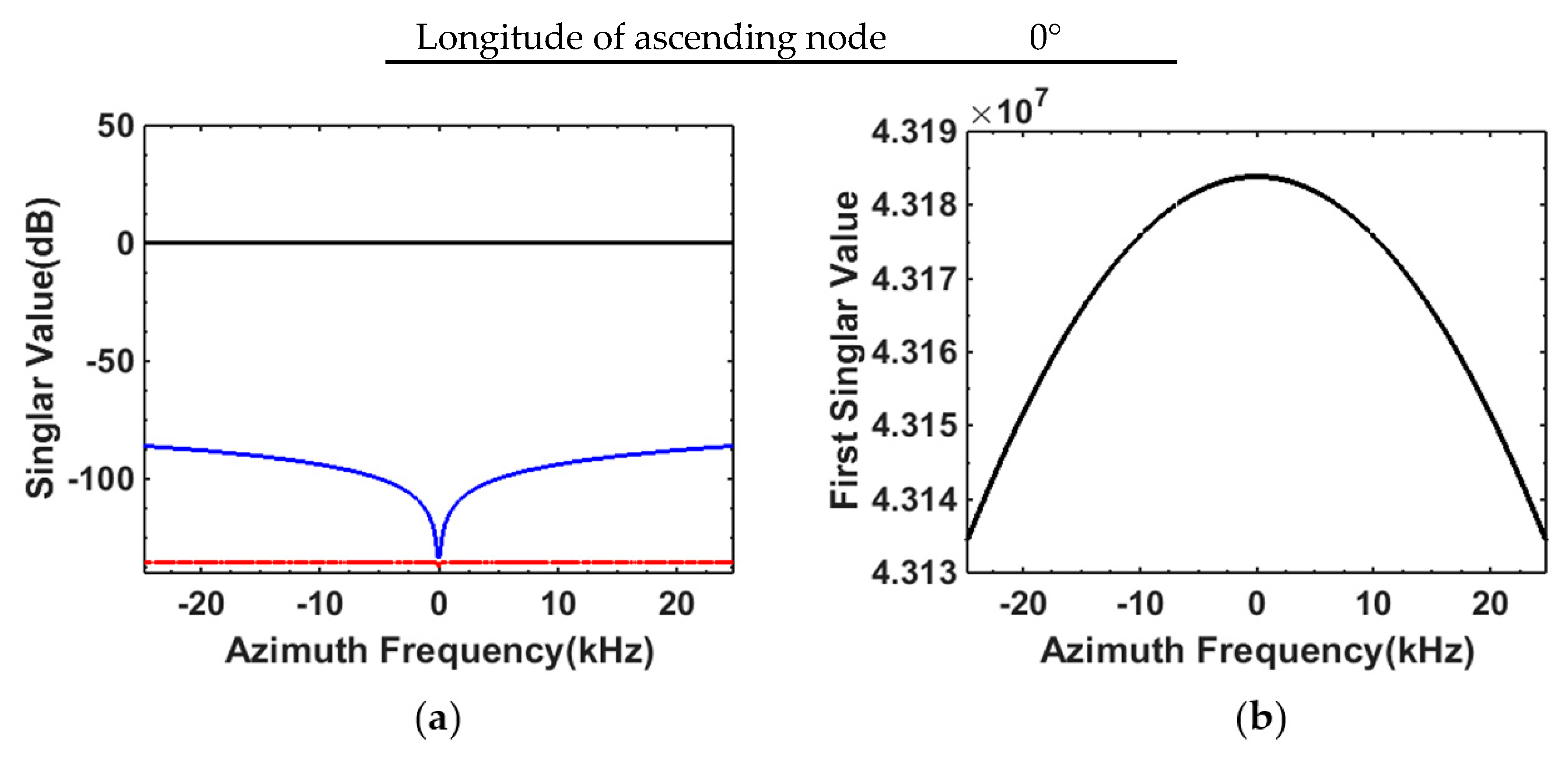
In Equation (38), superscript H denotes conjugate transpose operation, U_i is left singular vector matrix with size of N_r × N_r, Σ_i is an N_r × N_E matrix with singular values on the diagonal and V_i is the right singular vector matrix with size of N_E × N_E.

Figure 2 presents a demonstration of singular values. Figure 2a presents amplitudes of the first three singular values in decibels, which are normalized by the amplitude of the largest first singular value. Amplitudes of the first singular values in each azimuth frequency are shown in Figure 2b. Singular values in Figure 2 are acquired with the parameters in

Table 1. SAR system parameters.

Parameter Name	Value
Radar centre frequency	9.65 GHz
Signal bandwidth	1 GHz
Range sampling rate	1.2 GHz
Pulse Duration	8 μs
Azimuth processed bandwidth	49.43 kHz
Pulse repetition frequency	4.5 kHz
Look angle	35°
Synthetic aperture time	9 s
Range/Azimuth scene size	3 km/3 km
Closest slant range	629.913 km

and

Table 2. Orbit parameters.

Parameter Name	Value
Semi-major axis	6870.140 km
Eccentricity	0.0011
Inclination	97.423°
Argument of perigee	90°
Longitude of ascending node	0°

. As shown in Figure 2a, it is apparent that first singular values are much larger than second, and third singular values in each azimuth frequency. Consequently, the decomposition of Ψ_i can be approximated as follows:

$$SVD({\mathit{\Psi }}_{\mathit{i}})={\mathit{U}}_{\mathit{i}}{\mathit{\Sigma }}_{\mathit{i}}{\mathit{V}}_{\mathit{i}}^{\mathit{H}}\approx {\mathit{u}}_{\mathit{i},\mathbf{1}}{\sigma }_{i,1}{\mathit{v}}_{\mathit{i},\mathbf{1}}^{\mathit{H}}$$

(39)

In (39), u_i,1 denotes the first column of matrix U_i, σ_i,1 denotes the first singular value corresponding to Ψ_i and v_i,1 denotes the first column of matrix V_i.

Figure 2b illustrates that first singular values in different azimuth frequency are not constant and vary with azimuth frequency. In essence, performing SVD to Ψ_i in each f_η is intended to obtain numerical results of decomposition in Equation (32). By comparing Equation (32) with Equation (39) and considering information indicated in Figure 2b, it is reasonable that singular values should not be ignored in generating matrix for Stolt interpolation. 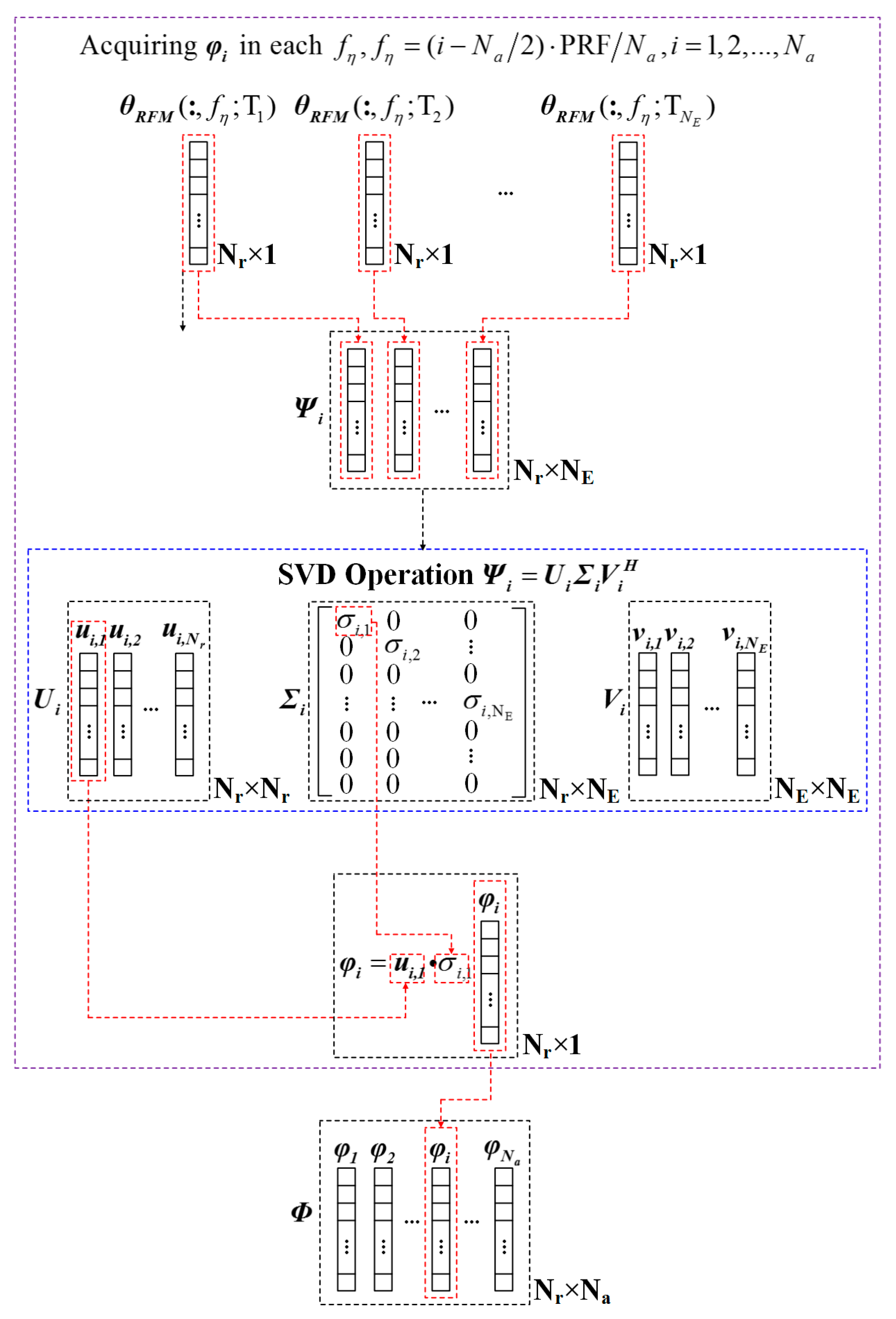Different from SVDS, modified RMA in this paper takes the singular value into consideration and acquires φ_i as follows:

$${\mathit{\phi }}_{\mathit{i}}={\mathit{u}}_{\mathit{i},\mathbf{1}}{\sigma }_{i,1}$$

(40)

After SVD operation in each f_η, the obtained φ_i can be arrayed to form a matrix as follows:

$$\mathit{\Phi }=\left[{\mathit{\phi }}_1,{\mathit{\phi }}_2,\dots ,{\mathit{\phi }}_i,\dots ,{\mathit{\phi }}_{N_a}\right]$$

(41)

The procedure of acquiring matrix Φ is presented in Figure 3. And Φ is a matrix with size of N_r × N_a.

The connection between the decomposition in Equation (32) and the decomposition in Equation (39) can be presented as follows:

$$\begin{array}{ll}{\mathit{\theta }}_{\mathit{RFM}}\left(:,f_{\eta };{\mathrm{T}}_1\right)& =-2\pi \mathit{\beta }(:,f_{\eta })\cdot 2\mathit{\gamma }(f_{\eta };{\mathrm{T}}_1)/c\\ & \approx {\mathit{u}}_{\mathit{i},\mathbf{1}}•{\sigma }_{i,1}•{\mathit{v}}_{\mathit{i},\mathbf{1}}^{\mathit{H}}\{1\}\\ & =-2\pi \frac{{\mathit{u}}_{\mathit{i},\mathbf{1}}•{\sigma }_{i,1}}{\alpha }\cdot \frac{2\alpha •{\mathit{v}}_{\mathit{i},\mathbf{1}}^{\mathit{H}}\{1\}}{c}\end{array}$$

(42)

$$\mathit{\beta }(:,f_{\eta })\approx \frac{{\mathit{u}}_{\mathit{i},\mathbf{1}}•{\sigma }_{i,1}}{\alpha }=\frac{{\mathit{\phi }}_{\mathit{i}}}{\alpha }$$

(43)

$$\mathit{\gamma }(f_{\eta };{\mathrm{T}}_1)\approx \alpha •{\mathit{v}}_{\mathit{i},\mathbf{1}}^{\mathit{H}}\{1\}$$

(44)

In Equation (42), θ_RFM(:,f_η;T₁) denotes any column in θ_RFM of target T₁, ${\mathit{v}}_{\mathit{i},\mathbf{1}}^{\mathit{H}}\{1\}$ denotes the first element in ${\mathit{v}}_{\mathit{i},\mathbf{1}}^{\mathit{H}}$ and α is a constant for associating the decomposition in Equation (32) with decomposition in Equation (39). As α is a constant, the interpolation coordinates calculated from Φ is the same as the interpolation coordinates calculated from β. Therefore, the matrix Φ is able to calculate interpolation coordinates for Stolt interpolation. As a result, acquisition and derivation of reference function and Stolt interpolation coordinates in the Modified RMA have been presented in this part.

2.3. Modified Deramping-Based Approach

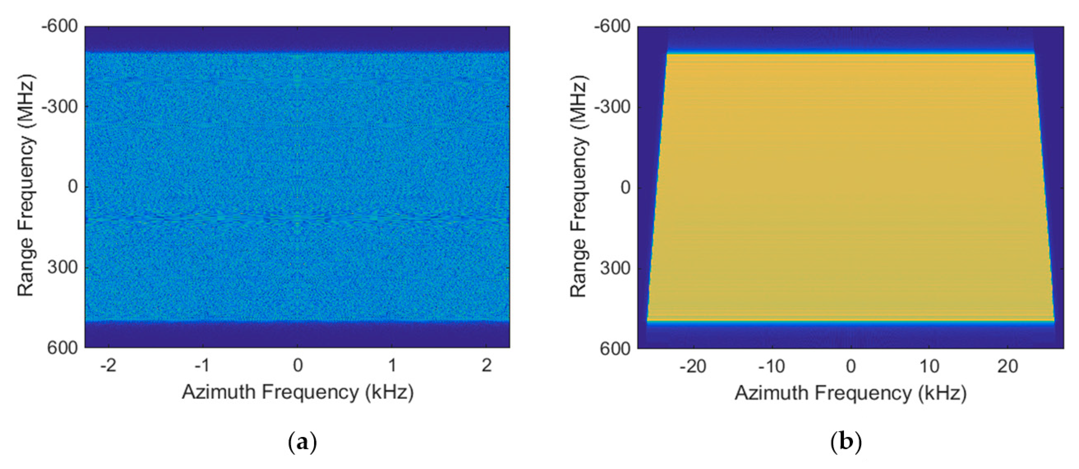
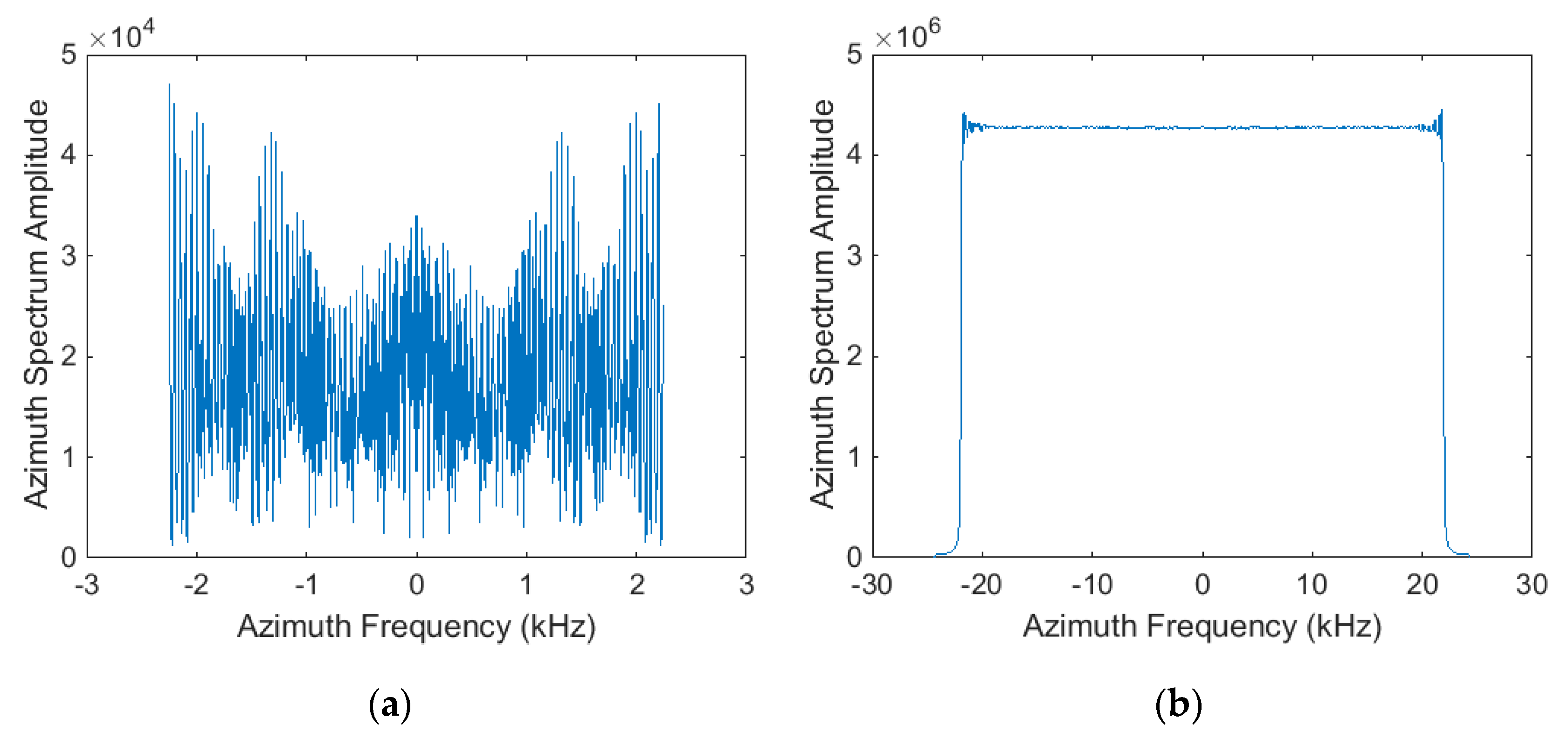
According to the Nyquist sampling theory, the pulse repetition frequency (PRF) should be larger than the azimuth bandwidth of echo data so as to avoid azimuth spectral aliasing problem. Nevertheless, in the scenario of high resolution spaceborne spotlight SAR, the PRF is usually smaller than the azimuth bandwidth. As a result, the phenomenon of azimuth spectral aliasing occurs in the situation of high resolution. Therefore, the traditional deramping-based approach is proposed to deal with the azimuth spectral aliasing problem under the consideration of uniform linear motion.

However, curved orbit is desired to be taken into consideration in spaceborne SAR when azimuth resolution achieves 0.14 m. Consequently, the traditional deramping-based approach is not suitable for the situation of curved orbit. Therefore, a modified deramping-based approach is proposed to solve azimuth spectral aliasing problem on curved orbit in this part. Orbital state vectors are utilized to estimate the Doppler parameter, the azimuth frequency modulation rate K_a, in the scenario of curved orbit. With the application of orbital state vectors, deramping-based approach is modified in order to accommodate the curved orbit in this paper.

The azimuth frequency modulation rate K_a can be obtained as follows when SAR platform is in uniform linear motion:

$$K_a==2v^2/\left(\lambda r\right)$$

(45)

In Equation (45), v is the velocity of the SAR platform, λ is the wavelength of carrier wave and r is the closest slant range.

In the scenario of curved orbit, K_a cannot be acquired with Equation (45). So as to solve this problem, orbital state vectors are introduced to the azimuth frequency modulation rate K_a in the scenario of curved orbit. The K_a can be acquired with orbital state vectors as follows:

$$K_a=-\frac{2}{\lambda }\left[\frac{\mathit{R}\circ \mathit{A}+\mathit{V}\circ \mathit{V}}{g_0}-\frac{{\left(\mathit{V}\circ \mathit{R}\right)}^2}{g_0^3}\right]$$

(46)

The R, V and A present relative position, velocity and acceleration 3-dimentional orbital state vectors between the radar and a target, respectively.

After K_a has been acquired, azimuth deramping can be implemented to s(τ,η) as follows:

$${\mathit{s}}^{\prime }(\tau ,\eta )=\mathit{s}(\tau ,\eta ){\ast }_{\mathrm{az}}\exp (j\mathsf{\pi }{K}_a{\eta }^2)$$

(47)

The *_az denotes convolution operation in azimuth direction. s(τ,η) is the echo data after demodulation to baseband.

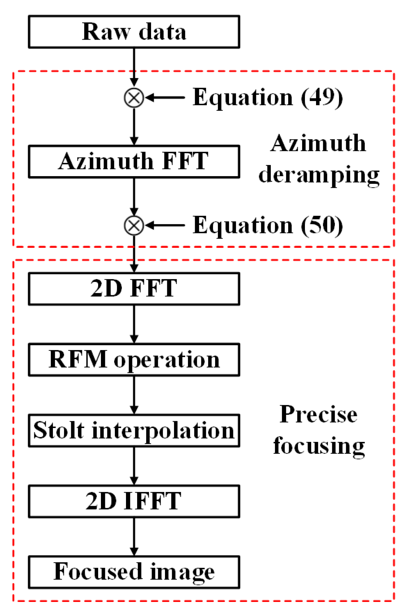
The convolution in Equation (47) can be implemented in an another approach which contains a chirp multiplication of the azimuth signal h₁(η), a subsequent FT operation and a residual phase h₂(η′) multiplication. In other words, the alternate way for azimuth convolution in Equation (47) can be expressed by Equation (48) as follows:

$${\mathit{s}}^{\prime }(\tau ,{\eta }^{\prime })={\mathit{h}}_{\mathbf{2}}({\eta }^{\prime })\cdot \mathrm{FFTa}\left[\mathit{s}(\tau ,\eta ){\mathit{h}}_{\mathbf{1}}(\eta )\right]$$

(48)

where the FFTa(•) denotes azimuth fast Fourier transform operation. Two quadratic phase signals, h₁(η) and h₂(η′), are defined in Equations (49) and (50) as follows:

$${\mathit{h}}_{\mathit{1}}(\eta )=\exp (j\mathsf{\pi }{K}_a{\eta }^2)$$

(49)

$${\mathit{h}}_{\mathit{2}}({\eta }^{\prime })=\exp \left[j\mathsf{\pi }{K}_a{\left({\eta }^{\prime }\right)}^2\right]$$

(50)

In Equations (49) and (50), the η and η′ are defined in Equations (51) and (52) as follows:

$$\eta =n/\mathrm{PRF},n=-N_a/2+1,\dots ,N_a/2$$

(51)

$${\eta }^{\prime }=n\cdot \mathrm{PRF}/\left(K_{a}P\right),n=-P/2+1,\dots ,P/2$$

(52)

As P > N_a, a zero padding operation of s(τ,η) in azimuth direction is required. As the η′ is determined by PRF, K_a and P, the P can be chosen according to the requirement of η′. In addition, the P can also be selected depending on the efficient implementation of FFT codes. Through application of modified deramping-based approach, azimuth spectral aliasing problem is solved.

2.4. Implementation of Proposed Method

The proposed method consists of modified RMA and modified deramping-based approach. The flowchart of the proposed method is illustrated in this part. As illustrated in Figure 4, the flowchart of the proposed method can be separated into two steps: azimuth deramping and precise focusing.

The step of azimuth deramping aims to solve the azimuth spectral aliasing problem in the scenario of curved orbit. In this step, modified deramping-based approach is implemented to SAR raw data according to Equation (48). The modified deramping-based approach is implemented through a phase multiplication of the signal h₁(η), a subsequent azimuth FT operation and another phase multiplication of the signal h₂(η′). With the implementation of modified deramping-based approach, the azimuth spectral aliasing problem has been solved.

After application of azimuth deramping, the step of precise focusing is utilized to obtain focused image. In this step, the raw data after azimuth deramping is firstly transformed into 2D frequency domain via 2D fast Fourier transform (FFT). Then, RFM operation is implemented to totally compensate the range migration of all targets at the reference range. The procedure of RFM operation is presented in Equation (30). After RFM operation, a residual phase exists for targets at other ranges. So as to cancel the residual phase, a subsequent Stolt interpolation is performed to cope with it. The Stolt interpolation is implemented in light of the matrix Φ. The procedure of obtaining matrix Φ is demonstrated in Figure 3 and is described in Section 2.2. After implementation of Stolt interpolation, 2D IFFT is operated to transform the data into the time domain and the data is eventually focused in time domain.

3. Results

In this section, point targets simulation is conducted to assess the effectiveness of the proposed method. The proposed method is compared with the generalized ωK in [13]. The results of simulation represent that the proposed method has smaller phase error and performs better than the generalized ωK when azimuth resolution achieves 0.14 m.

The simulation is under the consideration of monostatic spotlight spaceborne SAR with transmitting pulse chirp signal. The SAR system parameters for simulation are listed in Table 1. In simulation, the echo data is an 80,000 × 40,500 matrix with 80,000 range sampling points and 40,500 azimuth sampling pulses. After zero padding along azimuth direction in modified deramping-based approach, the size of data for processing becomes 80,000 × 44,500. The resolution of point target is expected to achieve 0.15 m and 0.14 m in range and azimuth direction, respectively. The swath width of scene is set as 3 km and 3 km in range and azimuth direction, respectively.

As the platform of SAR is considered to be a satellite in this paper, orbit parameters are taken into account in the simulation. A total of six independent parameters are required to describe the motion of a satellite around the earth [22]. The mean anomaly is time variant, which defines the position of satellite along the orbit. The other five constant orbit parameters are listed in Table 2. Orbit parameters in Table 2 are utilized in simulation so as to generate the curved orbit of spaceborne spotlight SAR. Nine point targets are positioned for simulation, which are labelled from T₁ to T₉. The distribution of point targets is shown in Figure 5.

The effectiveness of modified deramping-based approach is shown in Figure 6 and Figure 7. Figure 6a demonstrates 2D spectrum of single point target without application of modified deramping-based approach. And Figure 6b displays 2D spectrum of single point target with application of modified deramping-based approach. The row, which is at 0 Hz in the range frequency of each 2D spectrum, is chosen to illustrate the one dimensional (1D) azimuth profile of each 2D spectrum in Figure 6. Figure 7a shows the 1D azimuth profile of 2D spectrum without application of modified deramping-based approach. Figure 7b depicts the 1D azimuth profile of 2D spectrum with application of modified deramping-based approach. With the modified deramping-based approach, the PRF is enlarged from 4.5 kHz to 54.33 kHz. Meanwhile, the processed azimuth bandwidth is 49.43 kHz. Consequently, the enlarged PRF is larger than the azimuth spectrum bandwidth and the azimuth spectrum aliasing problem is solved with the application of modified deramping-based approach. As demonstrated in Figure 6b and Figure 7b, the azimuth spectrum aliasing problem is solved with the implementation of the modified deramping-based approach.

Figure 8a,b show the 2D spectrum phase error in the generalized ωK and the proposed method, respectively. The phase error is mainly caused by the numerical decomposition which is applied to the phase of the data after RFM operation. The phase errors shown in Figure 8a,b are obtained using parameters in Table 1 and Table 2. The first-order multivariable Taylor expansion, which is utilized for the numerical decomposition in the generalized ωK method, is responsible for the phase error of the generalized ωK. It is apparent that phase error in Figure 8a is larger than 0.8π rad at the edges of the spectrum with the parameters in Table 1 and Table 2. In other words, Figure 8a indicates that phase error of the generalized ωK is too large for SAR focusing when resolution is desired to achieve 0.15 m and 0.14 m in range and azimuth direction, respectively. As a result, such phase error in Figure 8a seriously degrades the imaging quality of SAR raw data. The SVD, which is used for numerical decomposition in the proposed method, is responsible for the phase error of the proposed method. In Figure 8b, phase error of the proposed method is less than 5 × 10⁻⁴ π rad. The phase error shown in Figure 8b indicates that the proposed method is more suitable for SAR focusing under the imaging requirements in this paper.

The imaging results of point targets via the generalized ωK and the proposed method are presented in Figure 9 and Figure 10. Nine target points are located according to the distribution in Figure 5. In Figure 9, imaging results of point targets acquired with the generalized ωK, which are labelled from T₁ to T₉, are depicted Figure 9a–i, respectively. In Figure 10, imaging results of point targets acquired with the proposed method, which are labelled from T₁ to T₉, are depicted Figure 10a–i, respectively.

As shown in Figure 9, it is that imaging results of T₁, T₂, T₃, T₇, T₈ and T₉ are not well-focused and suffer from azimuth defocusing. It can be concluded that the generalized ωK is unable to focus the echo data of spaceborne spotlight SAR when azimuth resolution attains 0.14 m. As illustrated in Figure 8a, such defocusing phenomenon in azimuth direction is caused by the unbearable phase error of the first-order multivariable Taylor expansion when resolution achieves 0.15 m and 0.14 m in range and azimuth direction. In contrast, the phase error of 2D spectrum in Figure 8b is much smaller than phase error in Figure 8a. Consequently, it is apparent that all the point targets presented in Figure 10 are focused much better than point targets in Figure 9. It can be concluded that the proposed method performs better than the generalized ωK when resolution achieves 0.15 m and 0.14 m in range and azimuth direction, with focused scene size of 3 km by 3 km.

4. Discussion

In order to further demonstrate the effectiveness of the proposed method, impulse response width (IRW), peak sidelobe ratio (PSLR) and integrated sidelobe Ratio (ISLR) are chosen as criteria for evaluating the quality of imaging results. The analysis for imaging results of point targets with the generalized ωK is listed in

Table 3. Analysis of results with the generalized ωK.

T	Range			Azimuth
	IRW (m)	PSLR (dB)	ISLR (dB)	IRW (m)	PSLR (dB)	ISLR (dB)
1	0.1334	−13.10	−10.43	0.1457	--	−5.73
2	0.1331	−13.09	−10.31	0.1459	--	−6.15
3	0.1336	−13.11	−10.40	0.1474	--	−5.67
4	0.1332	−13.03	−10.50	0.1298	−13.30	−9.69
5	0.1334	−13.24	−10.31	0.1272	−13.24	−10.31
6	0.1335	−13.02	−10.49	0.1269	−13.33	−10.32
7	0.1338	−13.32	−10.46	0.1330	--	−7.91
8	0.1339	−13.12	−10.31	0.1344	--	−7.51
9	0.1335	−13.22	−10.47	0.1331	--	−8.05

The ‘--’ denotes that azimuth defocusing makes measurement meaningless.

. And the analysis for imaging results of point targets via the proposed method is listed in

Table 4. Analysis of results with the proposed method.

T	Range			Azimuth
	IRW (m)	PSLR (dB)	ISLR (dB)	IRW (m)	PSLR (dB)	ISLR (dB)
1	0.1336	−13.08	−10.43	0.1302	−12.80	−9.61
2	0.1335	−13.23	−10.31	0.1273	−13.27	−10.23
3	0.1334	−13.05	−10.40	0.1274	−13.08	−10.18
4	0.1338	−13.32	−10.50	0.1282	−13.05	−9.85
5	0.1334	−13.23	−10.31	0.1273	−13.22	−10.24
6	0.1335	−13.28	−10.49	0.1279	−12.96	−9.94
7	0.1334	−13.25	−10.46	0.1280	−13.07	−9.83
8	0.1336	−13.23	−10.31	0.1282	−13.14	−10.18
9	0.1335	−13.26	−10.47	0.1281	−13.02	−9.85

.

In SAR processing, the IRW refers to as the image resolution. Namely, the IRW in both range and azimuth direction should satisfy the requirement of resolution. Furthermore, in order to guarantee the quality of the focused point target, PSLR should be less than −13 dB and ISLR should be about −10 dB.

The analysis in Table 3 shows that IRW, PSLR and ISLR of processed results obtained by the method in [13] satisfy the requirements of criteria in range direction. However, analysis in Table 3 indicates that IRW, PSLR and ISLR of processed results fail to satisfy the requirements of criteria in azimuth direction. As shown in Table 3, T₁, T₂ and T₃ fail to achieve 0.14 m in azimuth resolution. Meanwhile, the analysis in Table 3 is consistent with the imaging results in Figure 9 on the unsatisfactory focused performance in azimuth direction. In Table 3, the ‘--’ denotes that azimuth defocusing makes measurement of PSLR in azimuth direction meaningless. In comparison with the analysis in Table 3, Table 4 indicates that IRW, PSLR and ISLR of imaging results obtained by the proposed method almost satisfy the requirements of criteria in both range and azimuth direction. It is obvious that the proposed method has superior focusing performance in azimuth direction. Analysis in Table 4 and imaging results in Figure 10 verify that the proposed method performs better than the generalized ωK. In conclusion, the proposed method performs effectively on focusing raw data of high resolution spotlight spaceborne SAR when resolution achieves 0.15 m and 0.14 m in range and azimuth direction.

5. Conclusions

A method is proposed to deal with ultrahigh resolution spotlight spaceborne SAR imaging in this paper. The proposed method consists of modified RMA and modified deramping-based approach. The modified RMA method is developed for accommodating the scenario of curved orbit. The modified deramping-based approach is utilized to solve the azimuth spectral aliasing problem in curved orbit scenario. Point targets simulation and analysis operated on spaceborne spotlight SAR parameters validate the effectiveness of the proposed method. The focused results obtained by the proposed method generally obtain the expecting performance. Analysis demonstrates that resolution of focused results can achieve 0.15 m in range direction and 0.14 m in azimuth direction. Furthermore, the swath width of focused scene can achieve 3 km and 3 km in range and azimuth direction, respectively.