4.1. Dataset and Experimental Setup
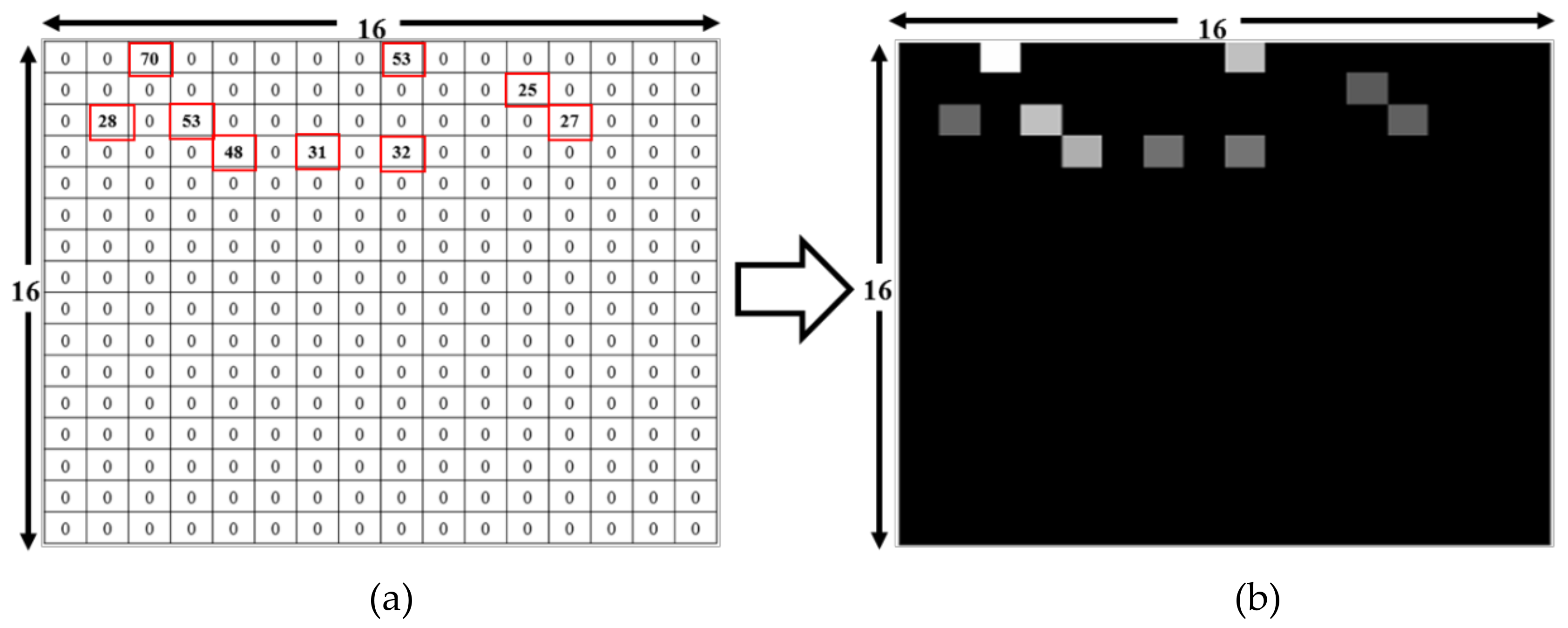
While the dataset collected during measurement was in a text format, the DL code was designed for a comma-separated values (CSV) input file. Given this, for training and testing, we converted the text files into a CSV file. These CSV files contained 257 columns and 74 RPs in the 257th column as labels. Data conversion was done using Python. The input for the file converter code (designed in Python) was folders containing text files.
To assess the validity of our approach, we created several datasets over four weeks. These were then used to assess which CNN layer is best to transfer knowledge from classification to indoor positioning as well as identifying the optimal classification algorithm. Results show that a relatively simple classification model fits the data well, producing ~95% generalization over a one-week period in the lab-based simulations with Scheme 1. The long-term introduction of new APs and drift in the existing APs need to be trained and learned.
To generate the dataset, the data is gathered over 7 days in four directions at the 74 RPs. It is then divided into four (Set 1: 7 days of data; Set 2: 5 days of data; Set 3: 3 days of data; and Set 4: 2 days of data), each then subdivided into separate cases based on the ratio of reference to trial data. For example, Set 1 (7 days of data) is divided into the three cases (6–1, 5–2 and 4–3). Datasets and cases are summarized in
Table 3. The dataset with 7 days of data has the maximum number of input files; accordingly, it has better overall test accuracy than the other sets as shown in [
11]. Therefore, Set 1/Case 1, which has six days of data for training and 1 day for testing, is used as the training and test dataset in our work.
RSSI fingerprint data collection and the final experiment were both performed on the 7th floor of the new engineering building at Dongguk University, Seoul, South Korea, shown in
Figure 15.
4.2. Hyperparameter Settings
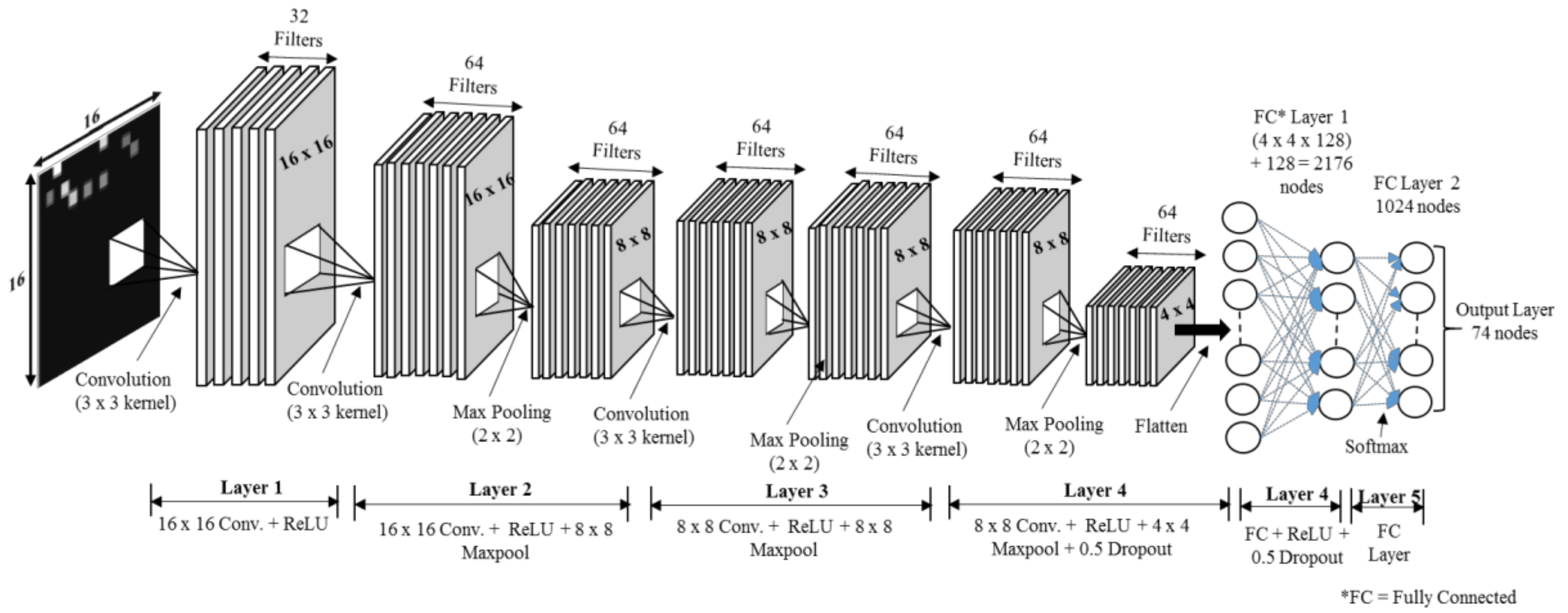
We trained the data on a network with different convolutional layers to find the best architecture. In each architecture, we adjusted the filter size, number of feature maps, pooling size, learning rate and batch size in the hyperparameter tuning process to retain the best configuration. We chose the best architecture with the best parameter setting as the final configuration.
Table 4 shows the list of hyperparameters and their candidate values. The values in bold reflects the best hyperparameter setting for our CNN model.
To analyse the effect of the number of layers, the CNN-based classifier was applied with different numbers of layers. The network with four convolutional layers outperformed others in all activities. The reason lies in the fact that networks with fewer than four convolutional layers are not complex enough to extract the appropriate features for activity recognition, whereas networks with four convolutional layers tend to cause over-fitting due to the structure complexity. Four convolutional layers are just enough to obtain good performance. The three-convolutional-layer network gives an accuracy of 91.32; however, the loss is higher compared to other layer networks. The loss in the setting signifies how well the CNN classifier learns from the training images to predict the test image correctly for each reference point. Therefore, lower losses are ideal for the CNN classifier. The test accuracy indicates how many test images are identified correctly by their own reference points or by a margin of 1 or 2 reference points. A higher test accuracy is desirable in accuracy of positioning case, since it reflects least error between training and testing environments. The epoch number is set to 20 due to the fact that the size of the dataset is few megabytes; therefore, with minimum epoch value model acquires high test accuracy. After 20–30 epochs, the model starts to overfit the result, and thus the total test accuracy start decreasing.
A seven-layer model has a test accuracy of 92.92% with loss 1.10 greater than a four-layer model. To determine the most appropriate filter size, the classifier was applied with different filter sizes (the number of convolutional layers was set to four). When the filter size was larger than three, the performance decreased with the increase of the filter size. The problem of overfitting occurs as filter size increases to seven and eleven. Therefore, the filter size was set to three. The best performance for each activity was achieved when the feature map was set to 64. The classification achieved the best performance when the pooling size was set to two. After this point, the performance decreased with the increase of the pooling size. Therefore, the pooling size was set to two.
Table 4 shows that when the learning rate is less than 0.001, the algorithm achieves a steady and reliable performance, whereas a learning rate larger than 0.01 shows unstable results. The reason for the poor performance with a large learning rate is that the variables update too quickly to change to the proper gradient descent direction in a timely manner. However, a small learning rate with good performance is also not the best choice, because it results in a slow update of variables and leads to a slow training process. Therefore, the learning rate was set to 0.001. The activity increased as the batch size increased from 250 to 1000 and decreased as the batch size changed from 1000 to 2000. Therefore, the batch size was set to 1000. As shown in
Table 4, the value in bold is the best setting of each hyperparameter.
All CNN applications require a different hyperparameter setting best suited for each application model. To determine the best parameter setting for our RSSI-based indoor localization problem, the CNN applications were performed by changing the learning rate and batch size. In
Table 5, the value in bold is the best hyperparameter setting of each CNN application for RSSI-based positioning. The remaining hyperparameters of each application remained the same as their inbuilt by-default values.
The learning rate varied at 0.01, 0.001, 0.005 and 0.0001 with batch size 32, 64, 128 and 256, respectively. Once the CNN application achieves improved performance with a specific learning rate, then the batch size is altered for that learning rate. Hence, both parameters were set for each CNN application. For initial learning rate, the batch size is set to 32.
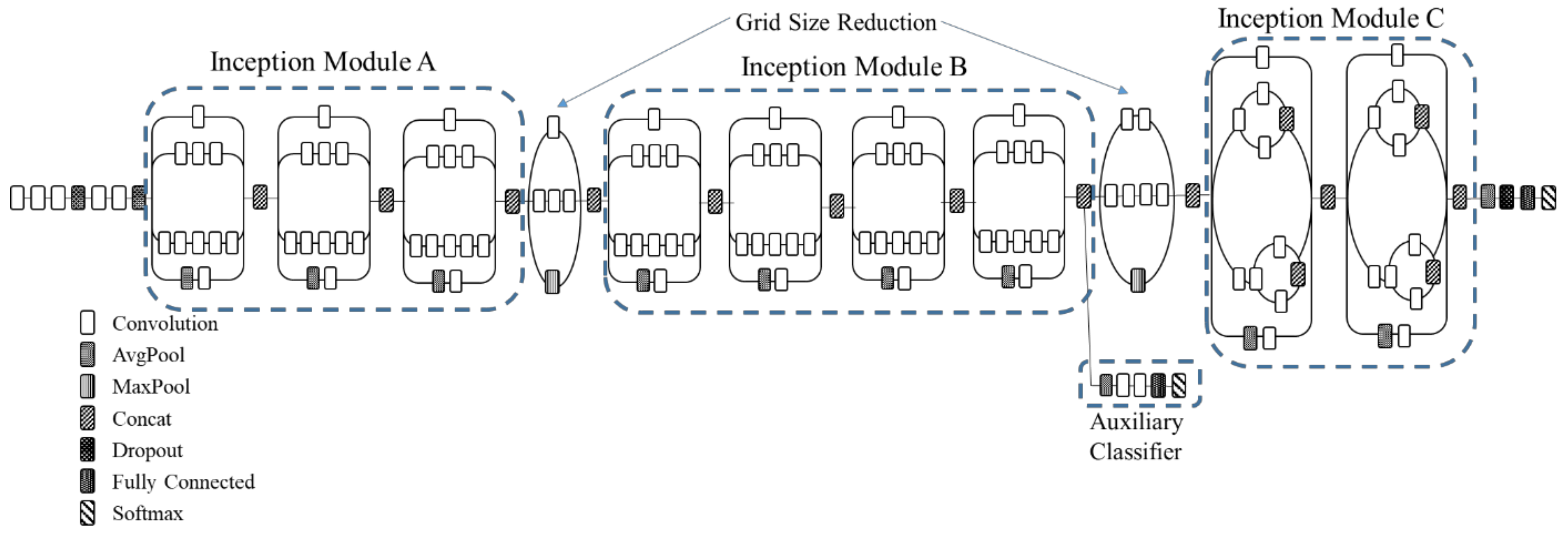
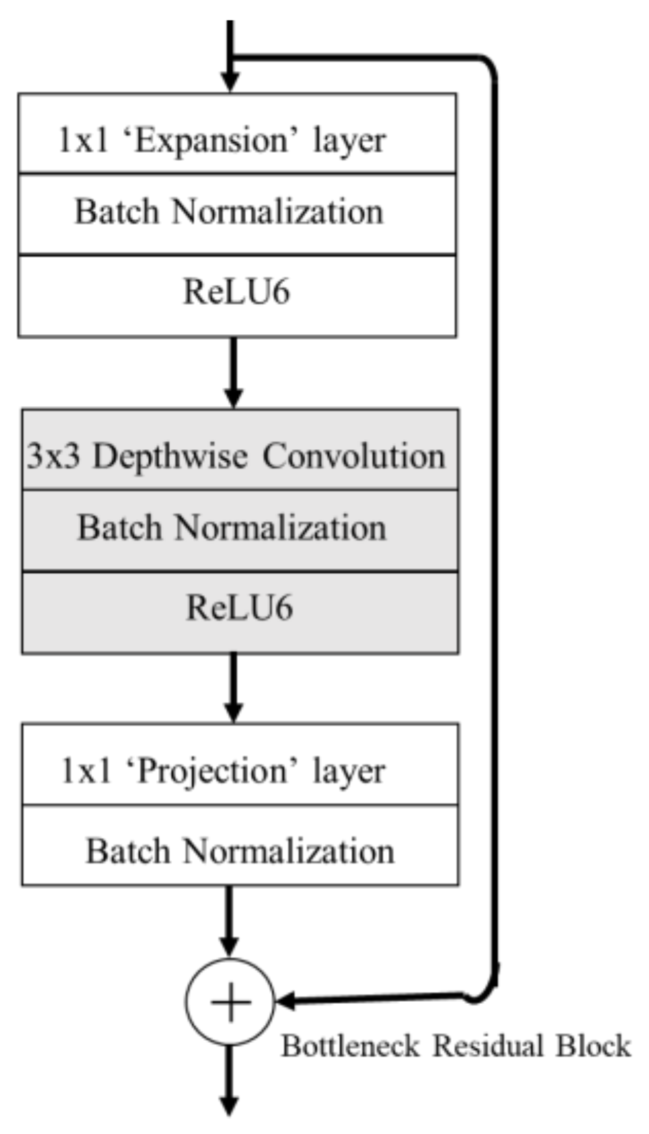
First, AlexNet performance is checked with the abovementioned learning rates. For learning rates 0.01 and 0.005, the loss values start with ~429 and remain the same after 20 epochs. At 0.0001, the initial loss value is 99.23 and test accuracy is highest, with 91.56% and loss value 79.85% after 5 epochs. At this learning rate, the batch size is varied, and batch size 64 achieved the highest test accuracy of 91.98%, for AlexNet. The optimum learning rate for ResNet is 0.0001 with initial loss value of 776.24, and after eight epochs the loss value is 212.98 with test accuracy 91.98%. At 0.005, the loss value reaches the highest at 12602.22, and test accuracy reduces to 6.79. At 0.0001 learning rate, batch size was tested for ResNet; batch size 32 produces the highest test accuracy of 89.74%, while batch size 256 produces ‘resource exhaust error’, which means the machine ran out of memory for allocating to the tensor. ZFNet gives the highest accuracy at 0.0001 learning rate, with a test accuracy of 91.71% and loss 46.76 after 5 epochs. The best-suited batch size for ZFNet is 64, with a test accuracy of 91.72%. In Inception v3 and MobileNet v2 the learning rate remained at 0.001. The total number of convolution layers in Inception v3 is 99, while in MobileNet v2 it is 56 (including the inverted residual blocks). Therefore, changing the learning rate exhausts the memory of the machine. The batch size for Inception v3 is 64 with a test accuracy of 87.09% at the 5th epoch, because the remaining batch size has overfitting results. For MobileNet v2, batch size 64 produces the highest test accuracy, with 88.54% and loss of 13.26 at the 3rd epoch. The initial loss value for MobileNet is 24.36.
4.3. Comparison with Other CNN Classification Methods
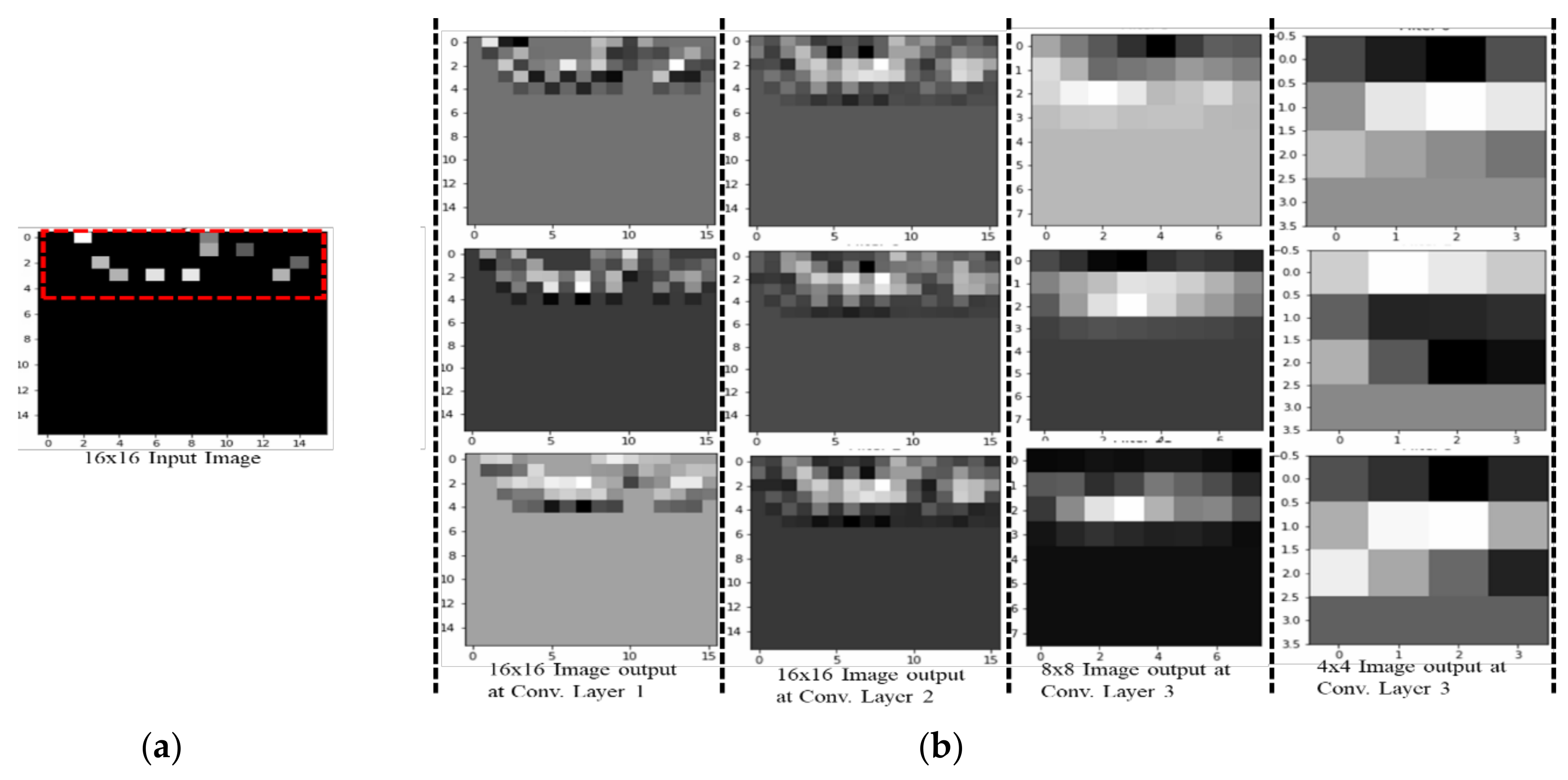
In this section, a detailed analysis of RSSI-based dataset localization performance is presented. To evaluate the performance of the prevailing CNNs, we investigated four aspects: validation accuracy, test accuracy, loss and time for each epoch. The accuracy curves for different CNN applications are shown in
Figure 16,
Figure 17,
Figure 18,
Figure 19,
Figure 20 and
Figure 21. As presented in
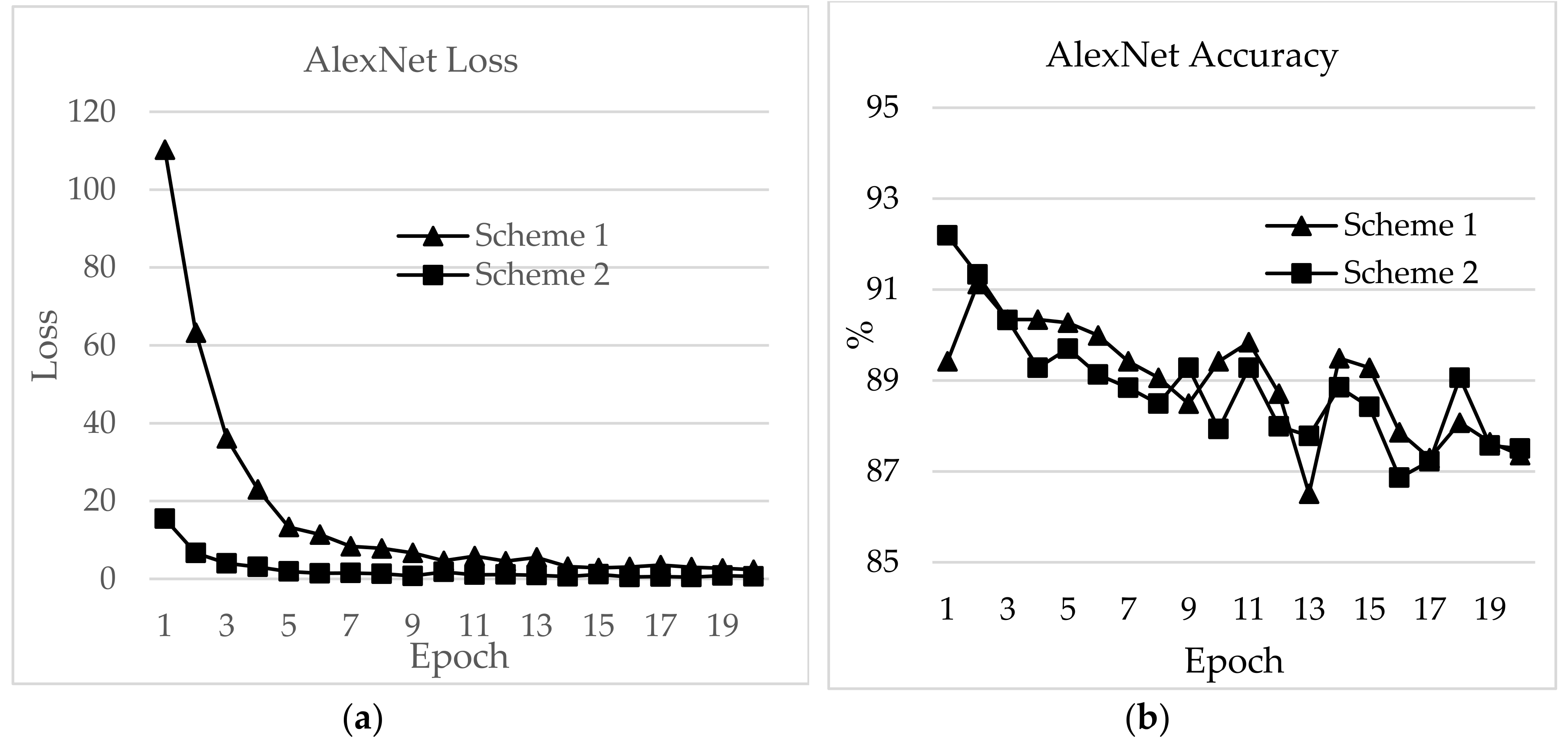
Figure 17, the features extracted from AlexNet are similar to the observation for the RSSI dataset. In
Figure 17, the loss for AlexNet is shown for both schemes. The initial loss and accuracy values were 110.29 and 89.42%, respectively, for Scheme 1 and 15.46 and 92.19%, respectively, for Scheme 2. AlexNet achieved a maximum accuracy of 91.12% for Scheme 1 and 91.19% for Scheme 2. This means that the network is well-suited as an RSSI-type fingerprinting dataset. The minimum loss values after 20 epochs were 2.37 and 0.66 for Schemes 1 and 2, respectively. As presented in
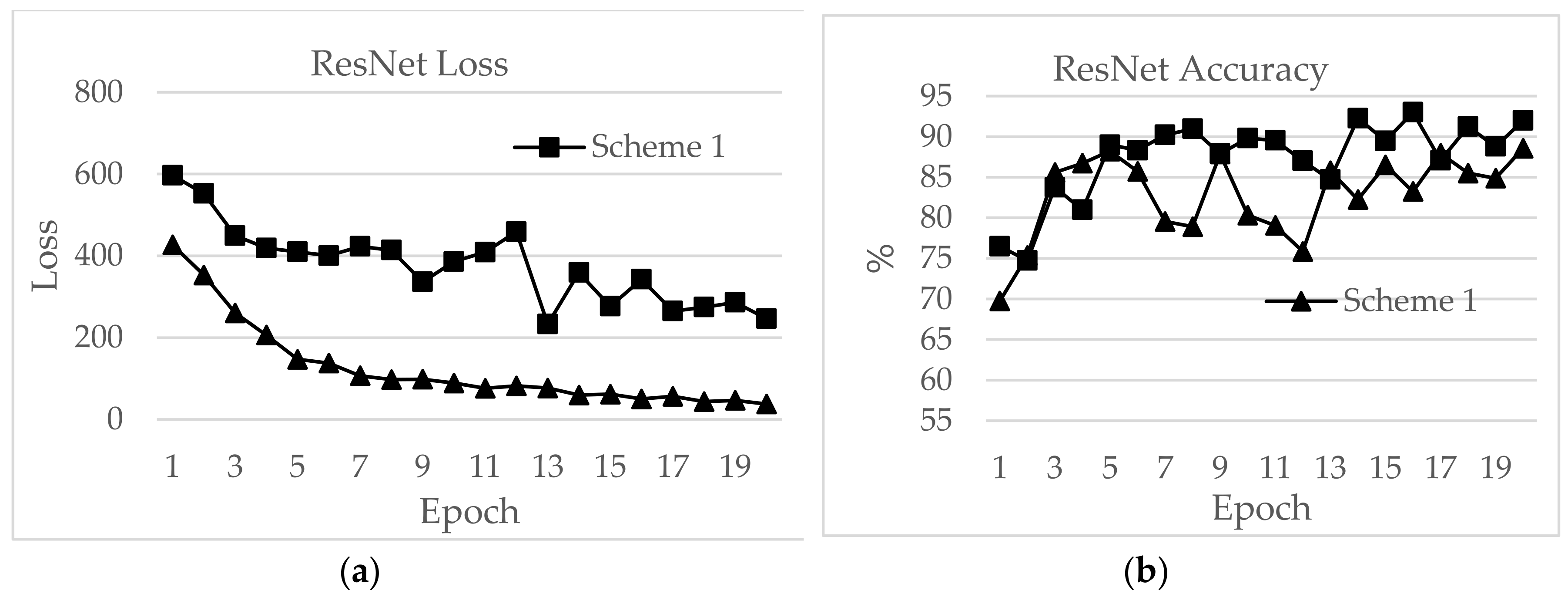
Figure 18, ResNet showed a maximum accuracy of 88.57% for Scheme 1 and 93.00% for Scheme 2. However, the losses after 20 epochs were 246.70 and 50.1 for Schemes 1 and 2, respectively. The accuracy further decreased even after the decrease of loss values. Therefore, the highest value reported for the ResNet model was the optimum value for RSSI-type datasets. The initial accuracy values for ResNet for Schemes 1 and 2 were 69.74% and 76.49%, respectively, and the losses were 596.81 and 427.04, respectively. As shown in
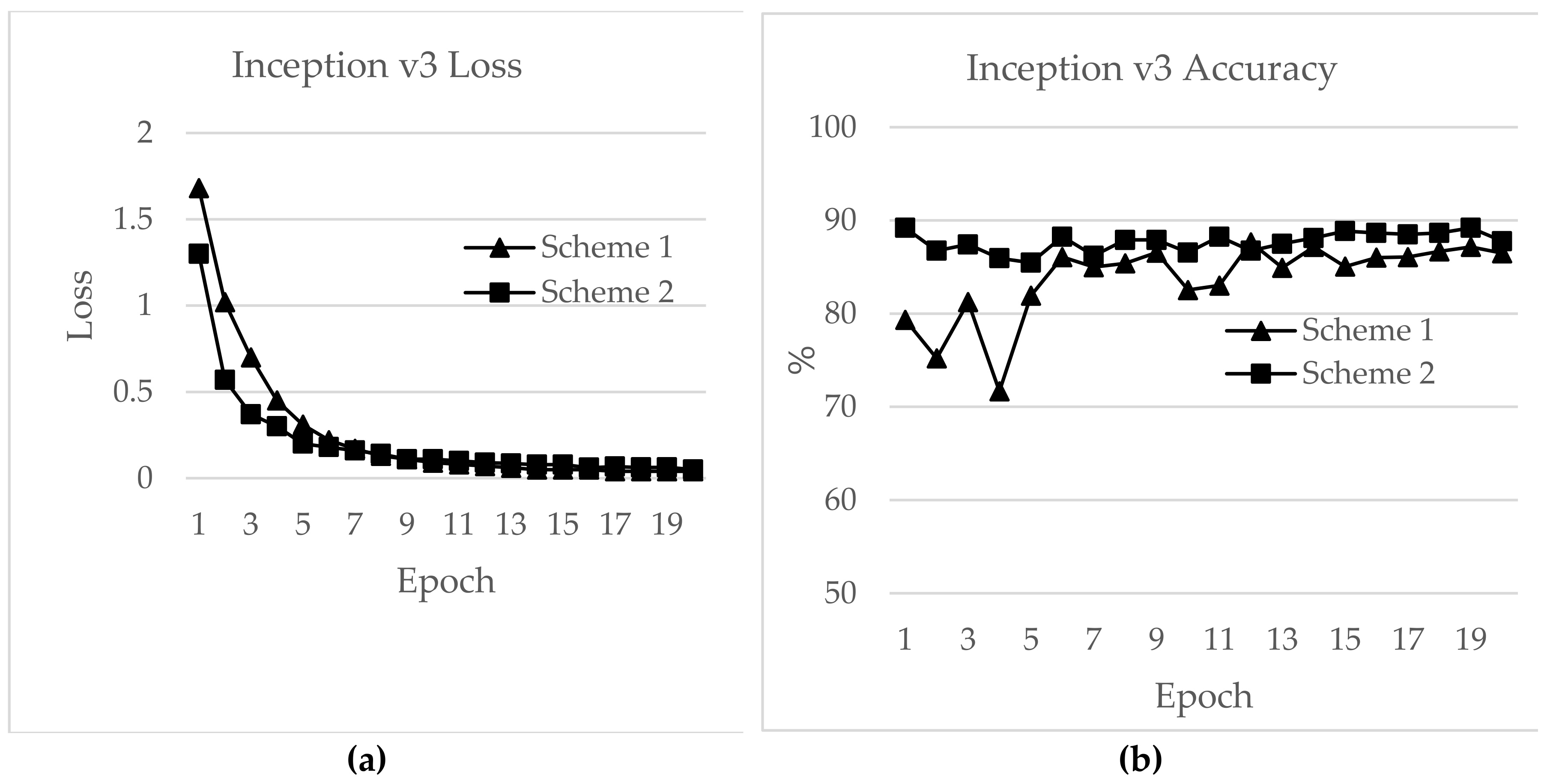
Figure 19, due to its simple architecture similar to AlexNet, ZFNet performed well for the RSSI dataset. Both training and testing showed accuracy values above 90%. The initial and highest accuracy values for ZFNet for Schemes 1 and 2 were 90.84% and 92.05%, respectively, with losses of 99.05 and 13.52, respectively. The accuracies after 20 epochs were 86.29% and 87.71%, with a loss of 1.76 and 0.48, respectively. Inception v3 was the lengthiest network to be trained and tested for the RSSI data type. As shown in
Figure 20, surprisingly, the highest accuracies achieved for this network for Schemes 1 and 2 were 87.16% and 89.20%, respectively. The loss values were 0.04 for Scheme 1 and 0.063 for Scheme 2. The initial loss values were 1.68 and 1.3 with accuracies of 79.35% and 89.02%, respectively. The final loss and accuracy values for Inception v3 after 20 epochs were 0.04 and 86.48%, respectively, for Scheme 1 and 0.05 and 87.77%, respectively, for Scheme 2.
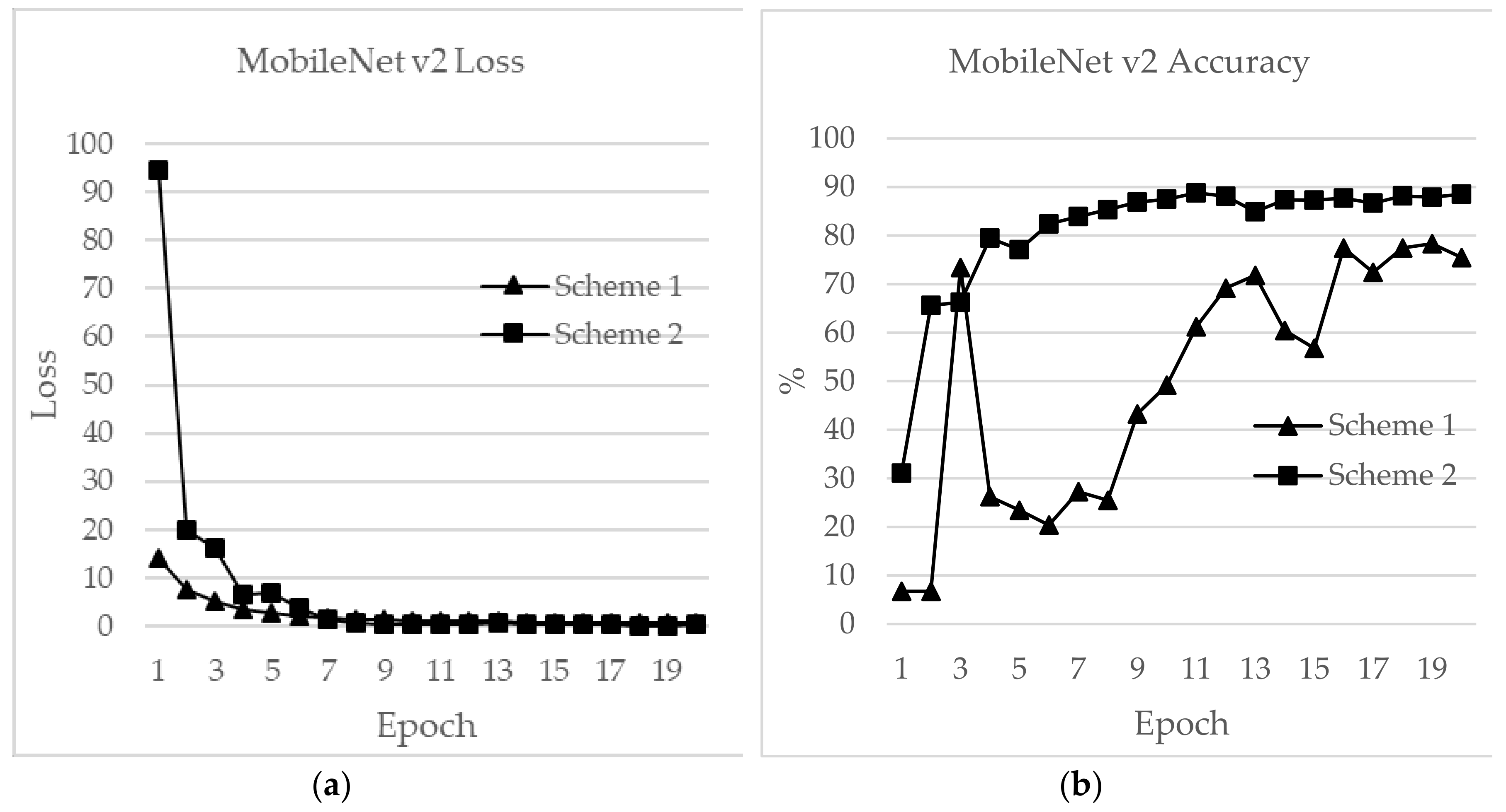
Figure 21 shows loss and accuracy for MobileNet v2. MobileNet v2 achieved the highest accuracy of 88.52%, for Scheme 2 and 78.33% for Scheme 1, which showed the lowest accuracy among the CNN applications. The initial and final loss values for MobileNet v2 were 19.95 and 0.6, respectively, for Scheme 1 and 94.45 and 0.25, respectively, for Scheme 2.
A performance comparison of a CNN application on the basis of four aspects was performed for the above models. As shown in
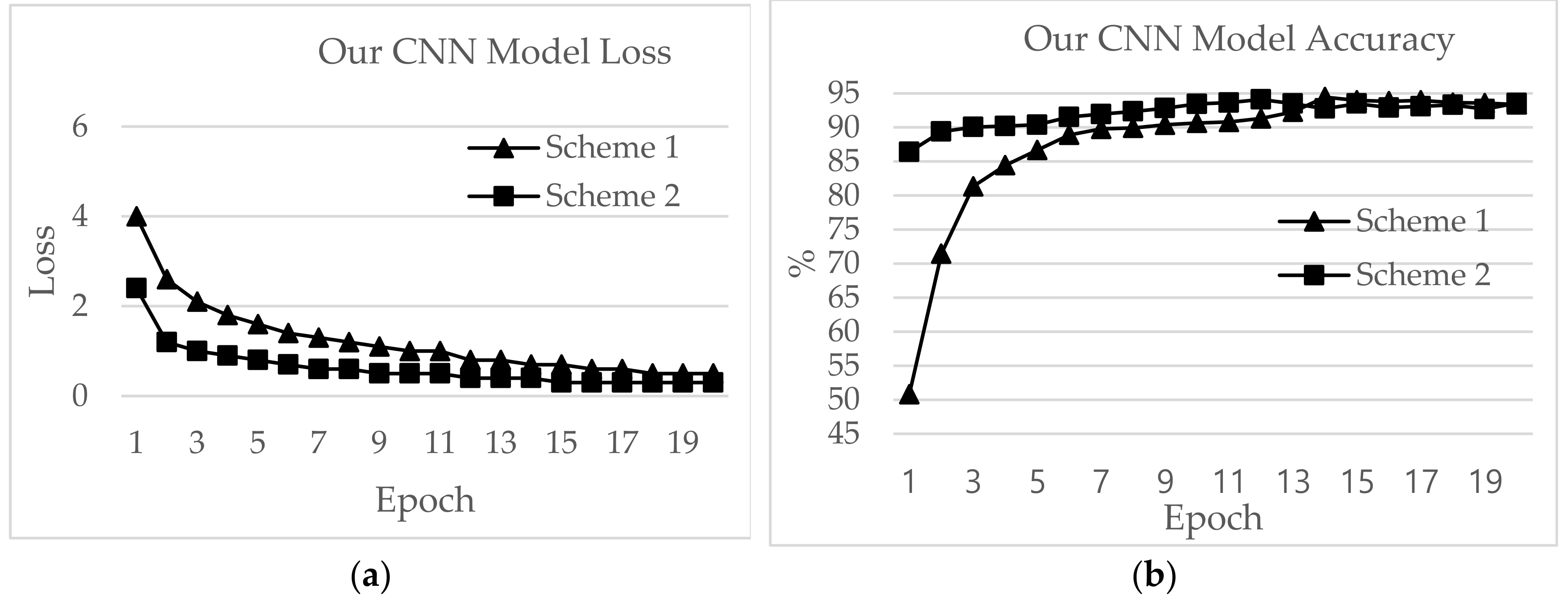
Table 6, our CNN model outperformed other applications in comparisons of epoch time, loss, validation and test accuracy.
The highest test accuracy achieved by our CNN model was 94.45% for the loss value of 0.7 with Scheme 1. Scheme 2 performed similarly, with a test accuracy of 94.11 and loss of 0.4. The epoch time was ~2 seconds for Scheme 1 and ~8 seconds for Scheme 2. The training accuracies were 69.87% and 86.99% for Schemes 1 and 2, respectively.
The second highest test accuracy was achieved by ResNet, with 93.00% for Scheme 2. The training accuracy was 96.44%. However, the epoch time was as high as 44.39 min while the loss was 56.54 for Scheme 2. For Scheme 1, the training accuracy was 81.88% and the test accuracy was 88.57%.
AlexNet performed best in terms of epoch time, with 1.41 and 6.78 min for Schemes 1 and 2, respectively, and test accuracies of 91.12% and 92.19%, respectively. The test accuracies for ZFNet were 90.83% and 92.05%, and the epoch times were 3.54 and 16.47 min for Schemes 1 and 2, respectively. The lowest test accuracy was exhibited by Inception v3, with 87.64% for Scheme 1 and 89.20% for Scheme 2. The epoch times for Schemes 1 and 2 were 4.17 and 20.38 minutes, and the training accuracies were 97.68% and 91.52%, respectively. MobileNet v2 showed epoch times of 4.15 min and 20.32 min with test accuracies of 78.33% and 88.52% for Schemes 1 and 2, respectively.
As shown in
Table 7, the number of RPs predicted accurately by the applications was called the zero-margin accuracy. Our CNN model had the highest zero-margin prediction, with 45.43% and 46.54% accuracy for Schemes 1 and 2, respectively. A two-meter difference between the actual and predicted RP was termed the one-margin accuracy. Our CNN model and ZFNet had similar outcomes, with 52.63% and 52.34% one-margin accuracy, respectively, for Scheme 1 and 51.23% and 51.14%, respectively, for Scheme 2. A difference of four meters between the predicted and actual outputs was called the two-margin accuracy. The highest two-margin accuracy was shown by our CNN model, with 94.45% and 94.11% for Schemes 1 and 2, respectively. The lowest two-margin accuracy was shown by MobileNet v2, with 78.33% and 88.52% for Schemes 1 and 2, respectively.
An indoor localization system is best evaluated on the basis of performance statistics using the mean value, variations and standard deviation. The mean is the total number of errors in meter units for indoor localization and is best if closest to zero. As shown in
Table 8, our CNN model achieved mean errors as low as 1.44 m and 1.48 m for Schemes 1 and 2, respectively, with standard deviations of 2.12 m and 2.35 m, respectively. AlexNet performed the best among the other CNN applications, with means of 1.80 and 1.67 m and standard deviations of 2.42 and 2.55 m for Schemes 1 and 2, respectively. Inception v3 showed mean errors of 4.39 and 4.23 m, standard deviations of 8.19 and 7.57 m and variations of 67.06 and 57.34 m for Schemes 1 and 2, respectively. The highest mean error is shown by MobileNet v2, with 4.39 m and 4.23 m and standard deviations 8.19 m and 7.57 m for Schemes 1 and 2, respectively.
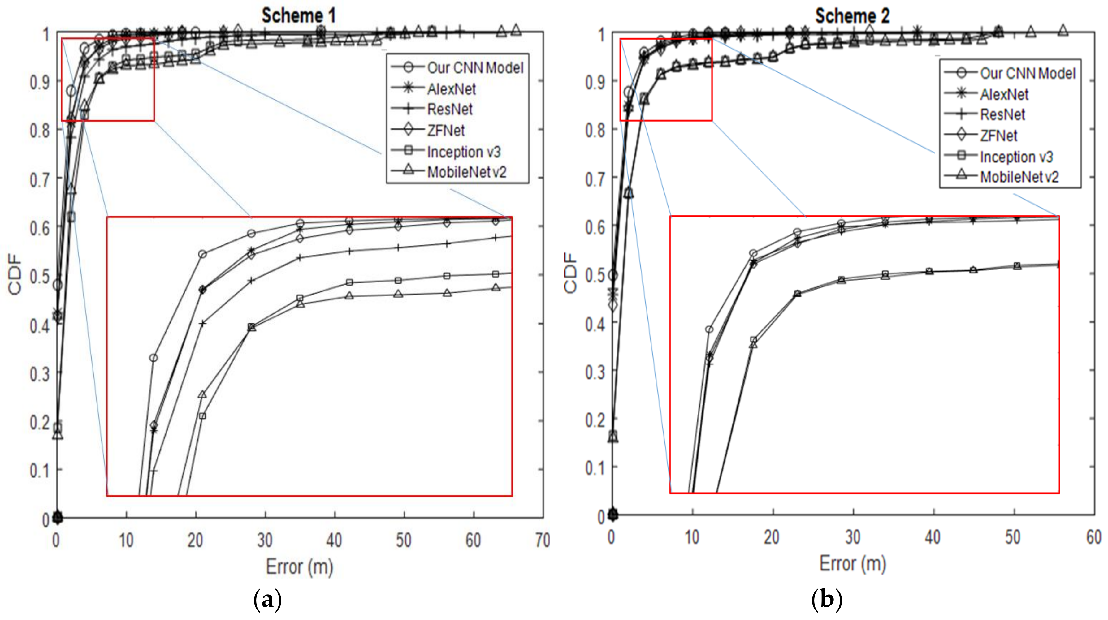
We also evaluated the effectiveness of indoor positioning (i.e., positioning accuracy), defined as the cumulative percentage of location error within a specified distance (
Figure 22). Our CNN model outperformed the other CNN applications over the entire range of the graph. Our CNN model with Schemes 1 and 2 did not differ greatly by positioning accuracy, such as in cases with error distance <5 m. Both schemes had probability values above 94% within <5 m error distance. However, for cumulative distribution functions over 94%, the positioning accuracy of Scheme 1 fell behind that of Scheme 2. Under 94%, the error distance for our CNN model was approximately 1.44 m, and Scheme 1 is ~0.03 m more accurate than Scheme 2. The gap between the two schemes increased gradually, and the error distance eventually rose to nearly 38 m. AlexNet and ZFNet achieved a probability of 91% within a 5-m error distance. Both had an error distance of 1.8 meters from the beginning and end of the graph with Scheme 1. ResNet lagged behind, with an error distance of 2.44 m and an accuracy of 88.57%. The gap eventually increased, and the error distance rose to 18 m for AlexNet, 26 m for ZFNet and 58 m for ResNet, which is the maximum value. Inception v3 had a maximum error distance of 4.13 m and 87.64% position accuracy within 5 m. The error distance for Inception v3 eventually increased to 54 m. With Scheme 2, the distance errors for AlexNet, ResNet and ZFNet became 1.7 m with ~92% accuracy for cumulative distribution functions. Therefore, the graphs for these models overlapped. The error distance eventually increased after 5 m. The error distance for AlexNet increased to 38 m, while that for ZFNet increased to 32 m. ResNet outperformed both models, with an error distance of up to 48 m. Inception v3 had an error distance of 4.10 m with an accuracy of 89.66%. After 5 m, the error distance for Inception v3 with Scheme 2 increased to 48 m. MobileNet v2 showed an error distance of 4.39 m with an accuracy of 78.38% for Scheme 1 and 4.23 m with 88.52% for Scheme 2.
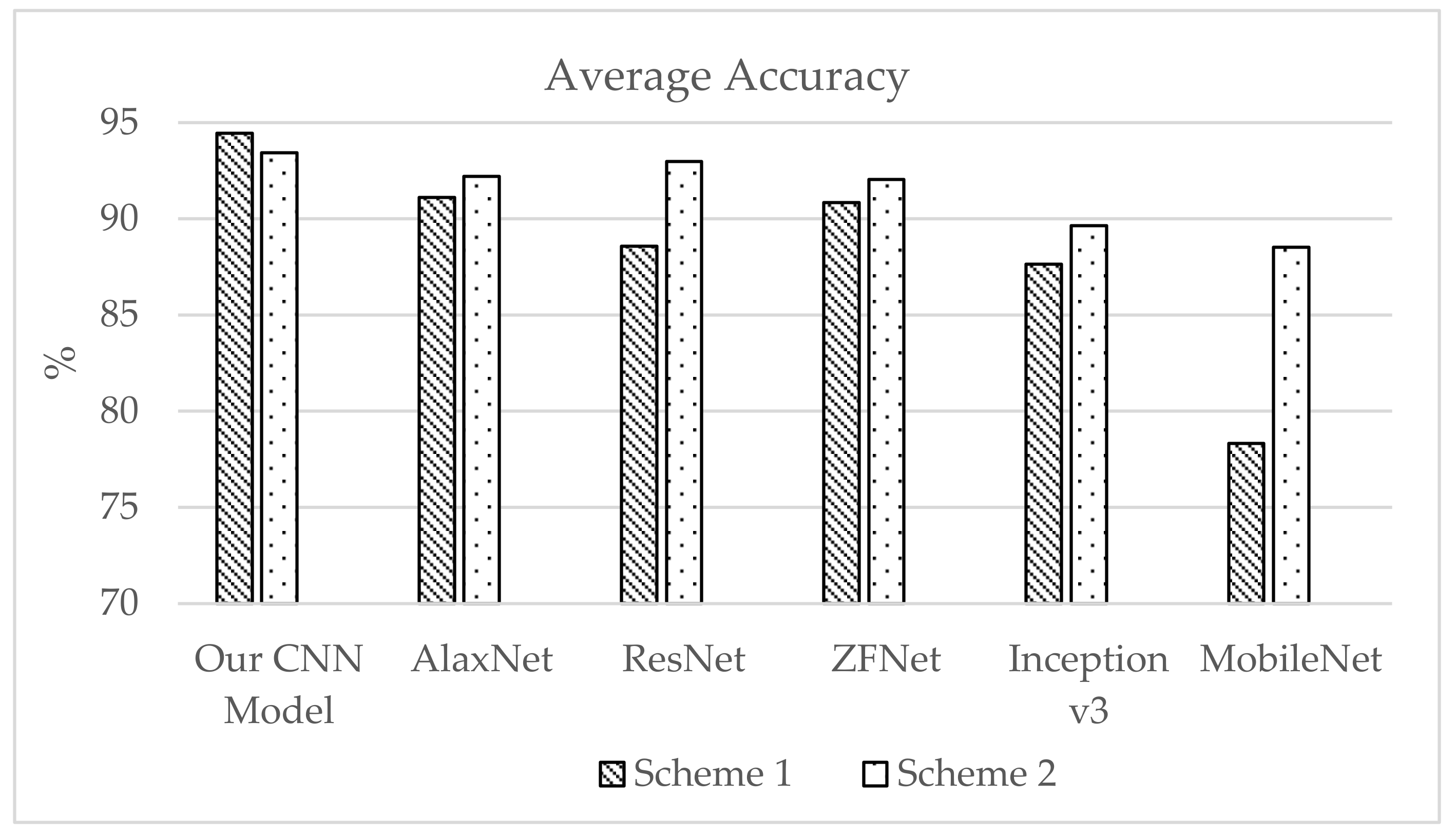
Figure 23 presents the average test accuracy with two lab test simulation results. Scheme 2 performed better with all CNN applications. The localization techniques proposed with our CNN model provide higher accuracy overall (i.e., a smaller error). We observed that CNN can fully exploit the additional measurements, making it a promising technique for environments with a high density of APs. In addition to the improved performance, our CNN model provides a fingerprinting approach that requires a less laborious offline calibration phase.


