The Model and Basic Equations
It is well known that the gravitational potential
, created by fluctuations in the matter density, is defined by scalar perturbations of the metric coefficients [
23] and that in the framework of General Relativity, it satisfies the linearized Einstein equation (see, e.g., [
24,
25]). Ignoring peculiar velocities, in the case of the
CDM cosmological model, this equation reads [
19,
20,
21]
where
(with
and
c being the Newtonian gravitational constant and the speed of light, respectively),
a is the scale factor, while
represents the Laplace operator in comoving coordinates. Here,
and
are the comoving mass density and its averaged value, respectively. As we operate within the
CDM model, matter is pressureless, and we consider it in the form of discrete point-like gravitating bodies with masses
to represent, e.g., galaxies. Therefore, the comoving mass density
The 0 subscript of
in Equation (
1) refers to the fact that peculiar velocities have been disregarded (see also [
26]).
The shifted gravitational potential
fulfils the equation
where the screening length [
19]
The presence of the term
in Equation (
1) (consequently,
in Equation (
4)) results in the Yukawa-type cutoff of the potential with the characteristic length
. The term
enters as a summand into energy-momentum fluctuations generating metric perturbations [
19].
In what follows, the overhat indicates that the gravitational potential is shifted. A significant bonus of working with the shifted potential is that it is now possible to employ the superposition principle in solving Equation (
4): once we find a solution for a single particle that is located at the center of Cartesian coordinates, we may immediately generalize it for a collection of particles at random positions.
We consider the space with chimney topology
, where the tori
and
have periods
and
along, e.g., the
x- and
y-axes, respectively. Hence, each gravitating body has its images positioned away from the original point in multiples of periods
and
along the corresponding axes. Now, let us place a particle with mass
m at the center of Cartesian coordinates. For the above indicated topology, the delta functions
and
may be presented as
which implicitly include the contribution from the images of the particle. Consequently, Equation (
4) for this particle reads
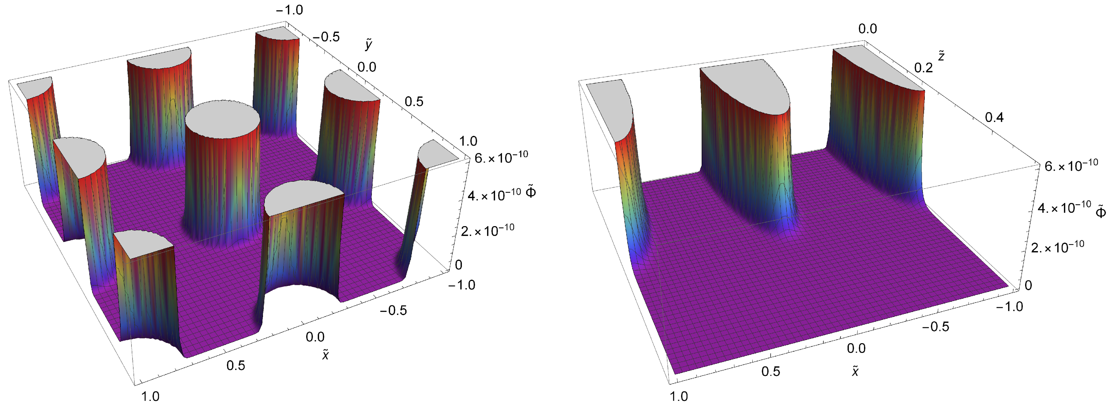
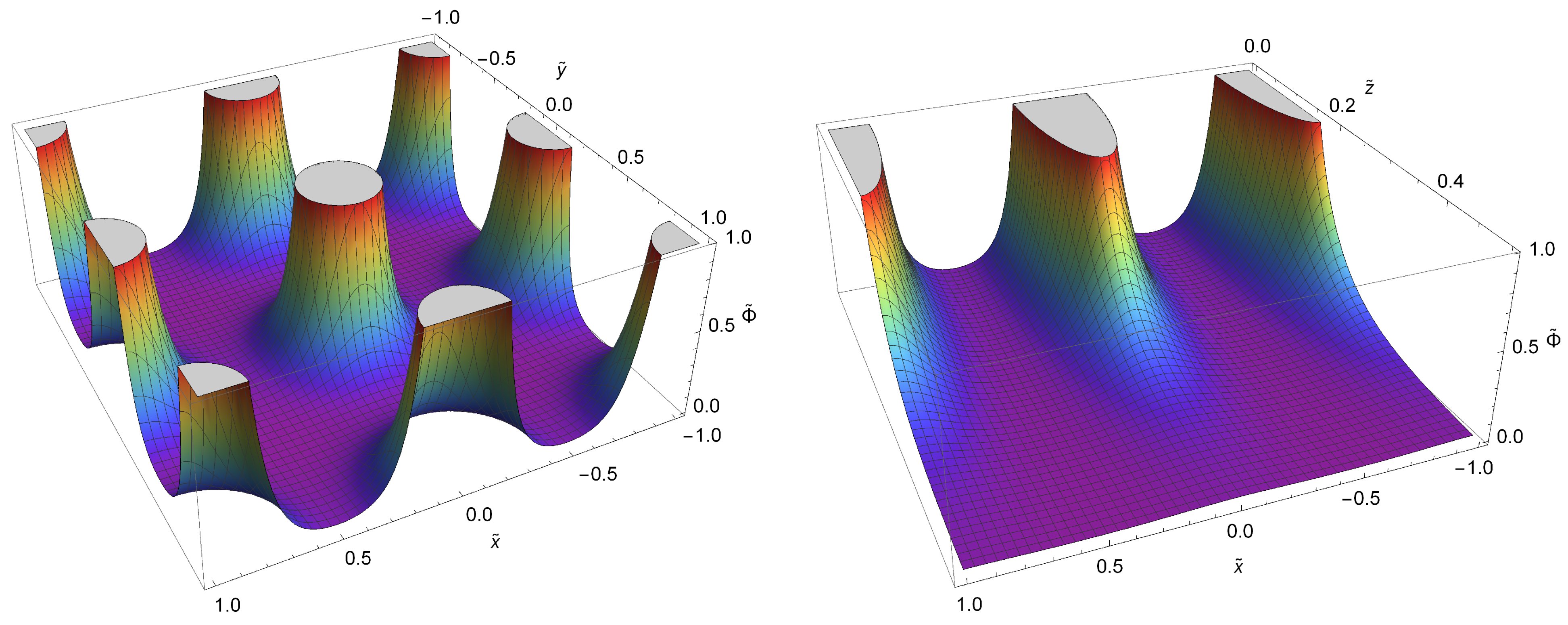
so, we are motivated to consider the solution
where the coefficients
satisfy the equation
Using the condition
, we can easily obtain the explicit expressions for the coefficients
, so that the shifted gravitational potential for the selected particle and all its images eventually reads
The above expression has the correct behavior in the Newtonian limit in the neighborhood of the considered particle, where it is no longer possible to distinguish between different (infinite and periodic) axes. For such regions, the summations in (
10) may be replaced by the integrals:
for
and
. Introducing the vectors
,
with the absolute values
and
, and assuming an angle
between them, we obtain
where
and
represent the physical distances, and the last integration is performed by using the formula 2.12.10(10) of [
27].
Evidently, for a system of randomly positioned gravitating bodies, we have
For linear fluctuations, the averaged value of this expression is equal to zero, as it should be (also see [
28]). Indeed,
and, hence, the spatial average of the total gravitational potential is
For the sake of simplicity, here we have considered the particular configuration in which all N bodies in the volume are assigned identical masses m.
Equation (
4) is of Helmholtz type and we can likewise solve it by considering the contribution of periodic images. In this case, the resulting expression consists of summed Yukawa potentials attributed to each one of them:
As we have noted previously, the peculiar motion of gravitating bodies is disregarded in Equation (
1) and, consequently, in (
4). Nevertheless, the significance of such a contribution has recently been pointed out in [
29], where the authors have also shown that peculiar velocities may be effectively restored by employing the effective screening length
(given by the formula (41) of [
29]) instead of the screening length
in Equations (
1) and (
4). Specifically, in the matter-dominated epoch, the two quantities
and
are related to one another as
. Returning to our formulation, the effect of peculiar motion is included by replacing
with
in the formulas (
10) and (
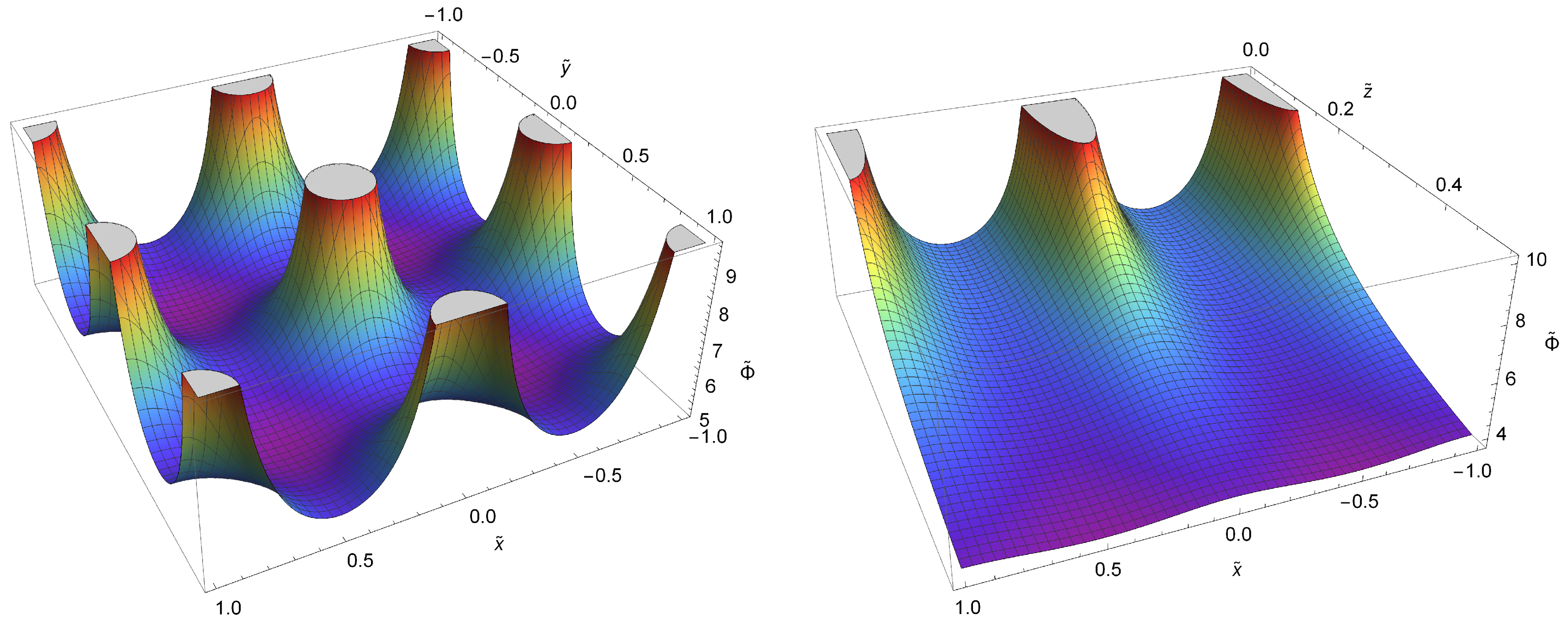
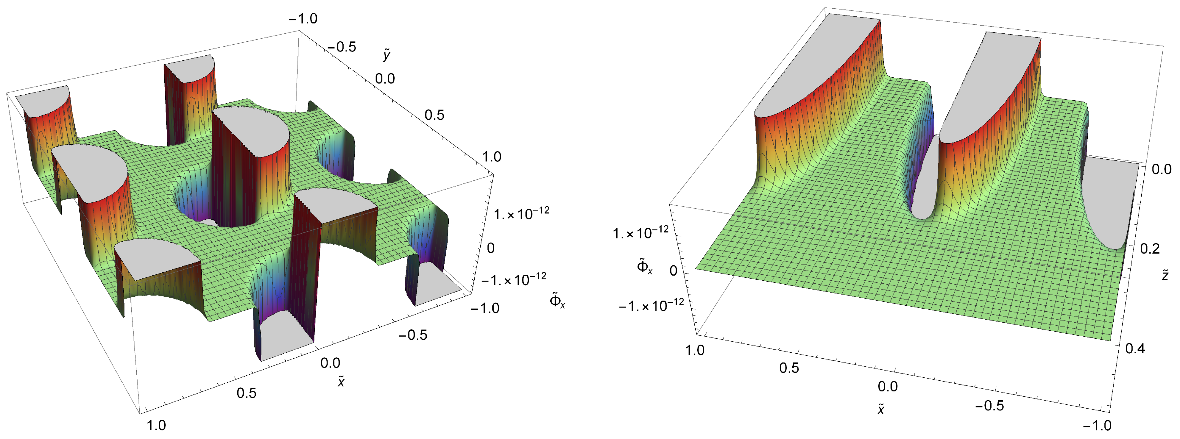
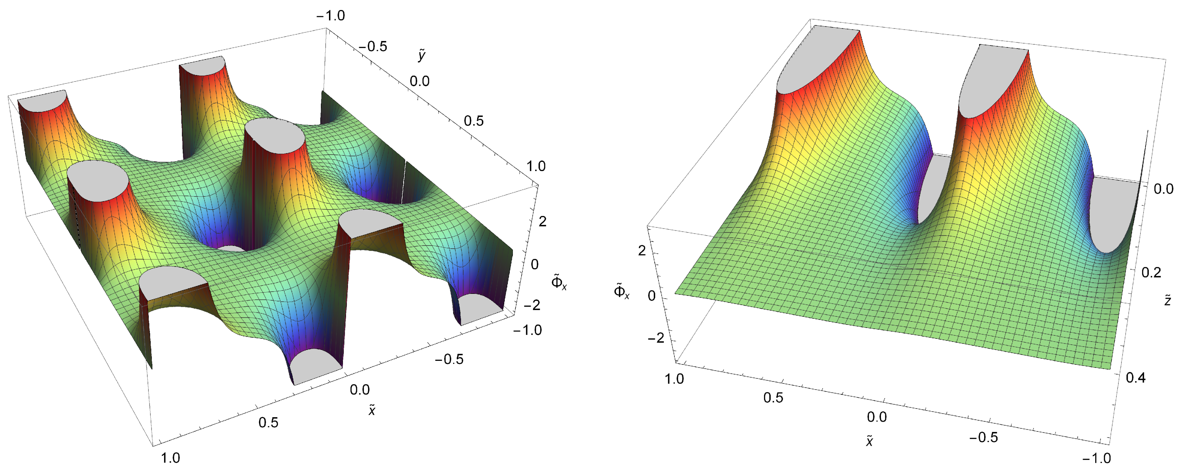
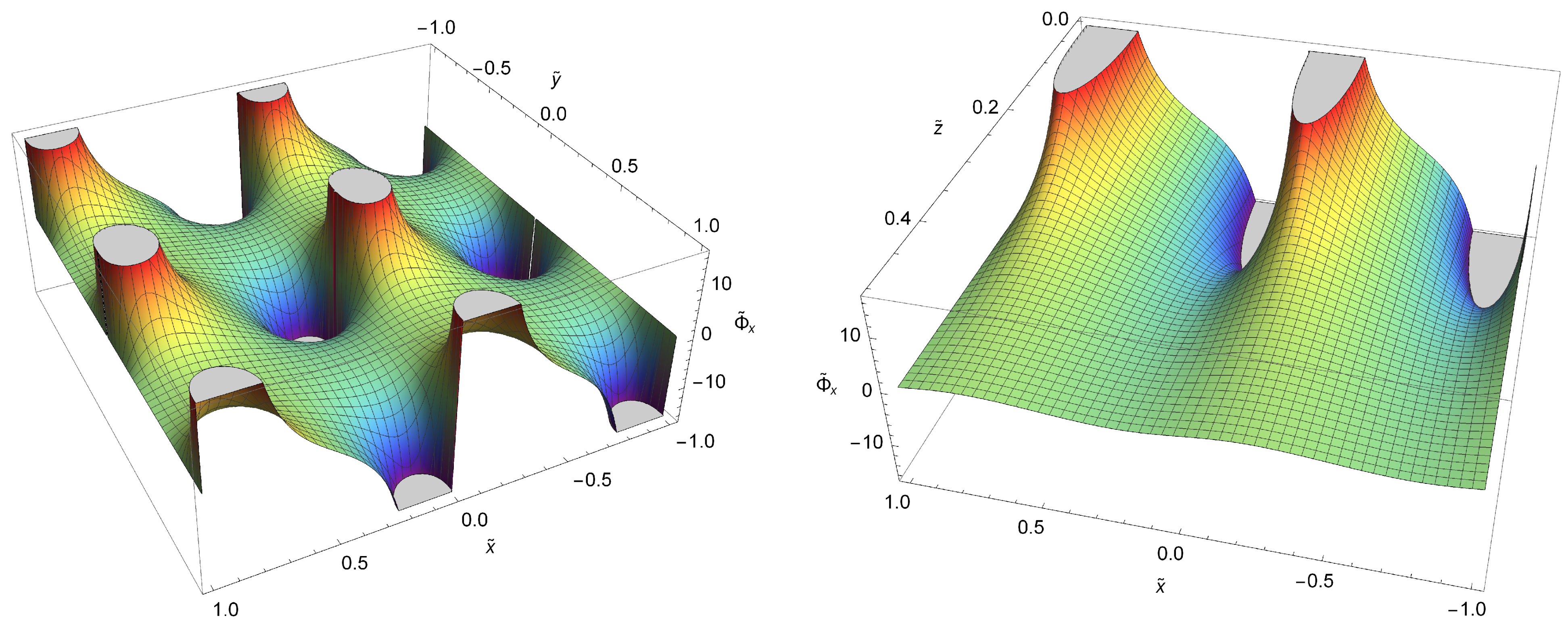
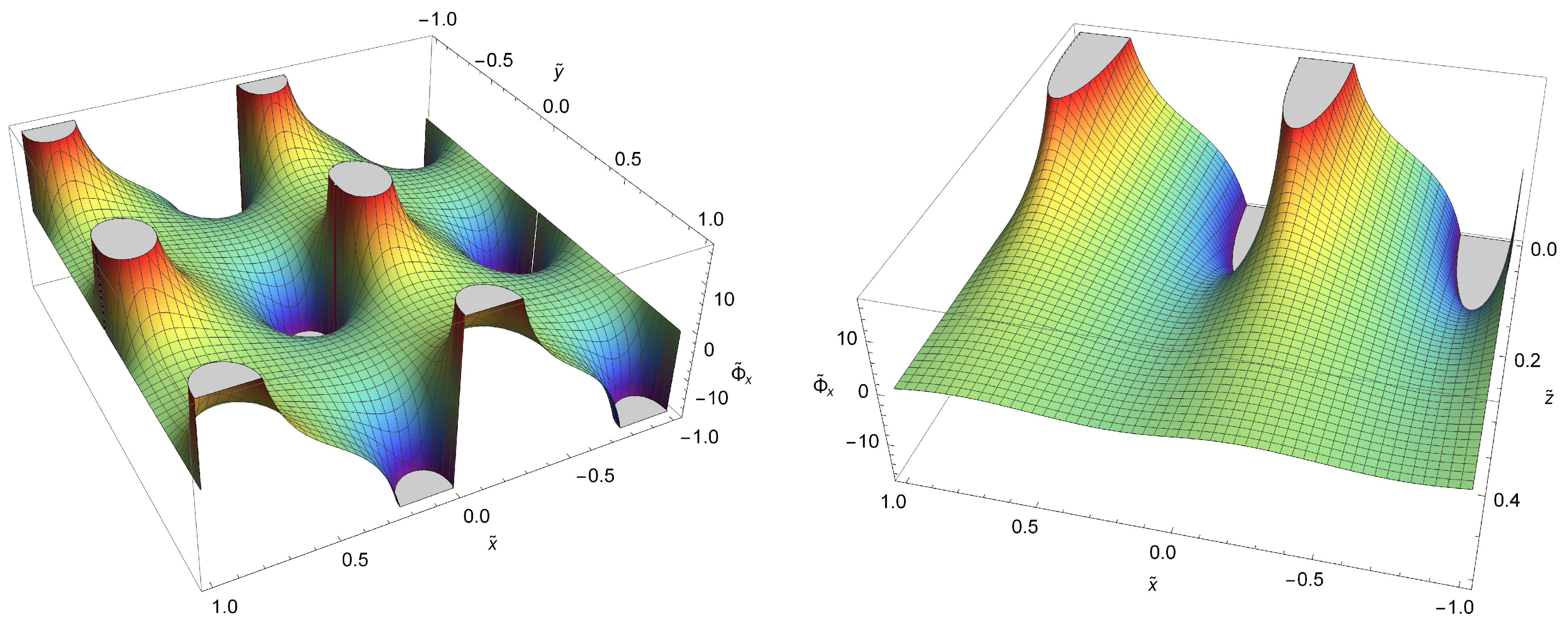
16), which yields
and
For simpler demonstration, we have assumed
and introduced the rescaled quantities
Two alternative solutions are labeled with the subscripts “cos” and “exp” in Equations (
17) and (
18). Now that the peculiar velocities are included in the calculations, the 0 subscript is omitted in the new formulas.
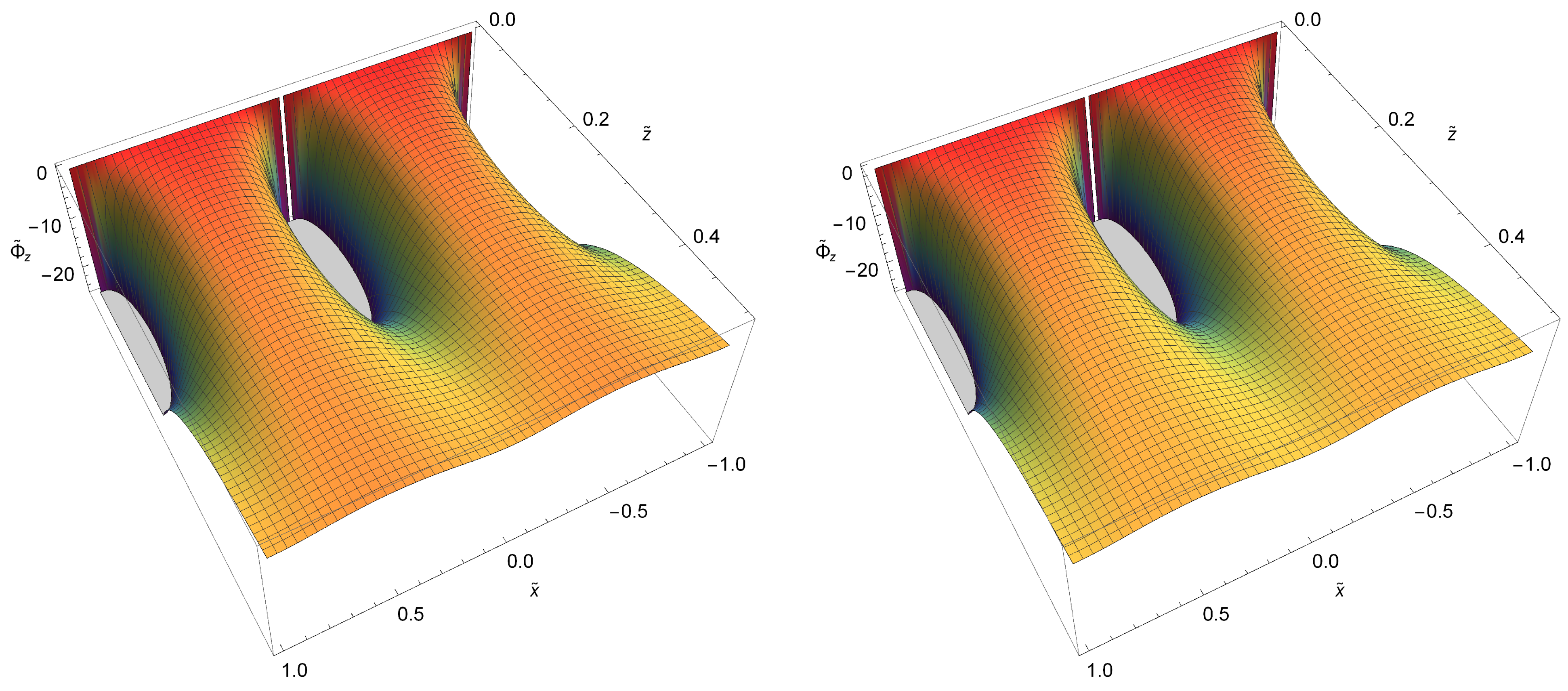
There is also a third way to express the gravitational potential for the given topology. Indeed, Yukawa-type interactions that are subject to periodic boundary conditions can be formulated via Ewald sums, so that the expression for the potential consists of two rapidly converging series, one in each of the real and Fourier spaces. The technique is commonly employed while modeling particle interactions in plasma and colloids, and, in such a context, the corresponding potential for quasi two-dimensional systems, i.e., three-dimensional systems with two-dimensional periodicity, has previously been derived in [
30,
31]. Being implemented in the cosmological setting considered in our paper, the discussed expression for the “Yukawa–Ewald” potential reads
where
and
In these formulas, erfc is the complementary error function and the free parameter
, as indicated in [
31], is to be chosen in such a way that a balanced interplay of computational cost and satisfactory precision is achieved. For definiteness, we set
equal to
.
In the forthcoming section, we will compare three expressions and present the optimum formula in view of its efficiency in use for numerical analysis.


