1. Introduction
Limestone is a significant resource available in Pakistan [
1] and is used to produce cement, concrete, road base, and dimension stone products [
2]. Since conventional exploration/prospecting practices are costly, time-consuming, are limited by physical access to hilly terrains, and prone to accumulating errors, remote sensing has been widely utilized in lithological/geological mapping [
3,
4,
5,
6,
7,
8,
9,
10]. Most minerals respond to near infrared (NIR), shortwave infrared (SWIR), and thermal infrared (TIR) wavelengths [
11,
12,
13]. Sedimentary rock units such as dolomite, quartzite, and limestone mainly respond to the TIR bands [
14,
15]. However, limestone also reflects the visible and NIR electromagnetic radiations while absorbing SWIR [
16]. A variety of remote sensing data sources are available from non-commercial (e.g., Landsat-8, ASTER, Sentinel-2) to commercial (SPOT, AVIRIS, WorldView–3) satellites. The spectral bands of ASTER L1T, Sentinel-2 MSI, Landsat-8/7 data sources have been useful for geological mapping and mineral exploration. The ASTER sensor has CaCO
3 absorption in SWIR and TIR bands [
16], while SWIR bands of Sentinel [
17] and SWIR and TIR bands of Landsat-8 [
5,
7,
18,
19,
20,
21,
22,
23] have also been useful in identifying and discriminating carbonate minerals. Individual bands in remote sensing images can produce detailed maps; however, it is a time-consuming process requiring manual comparison and interpretation through the naked eye and substantial expert knowledge [
24]. Conventionally, band ratios, derived on a trial and error basis, have been useful to map geology; e.g., ASTER bands 14/13 have been used for limestone mapping [
16,
25]. However, environmental factors, instrumental limitations, and mixed albedo from different lithologies invite robust data mining and machine-learning algorithms (MLAs) to reveal relevant patterns for generating reliable geological maps [
26].
Accuracies of machine-learning algorithms (MLAs) rely on careful selection of data labels, which can be flawed due to lower spatial resolution, misregistration, update delay, or lithological complexity [
27]. Since data labeling/annotation is a significant challenge in achieving reliable mapping accuracy through MLAs [
27], post-classification field surveys must support classification accuracy. Algorithms prone to noise, such as classification and regression tree (CART) [
28], must be used with care compared to random forest (RF), which is relatively less sensitive, more generalized, and therefore, widely used for geological mapping [
29,
30]. However, CART can also outperform RF if training data are noise-free and labels are accurate [
28].
Data annotation/labels can be improved through fusion maps obtained by applying unsupervised techniques such as principal component analysis (PCA), Crosta technique, DS, and unsupervised clustering [
31,
32,
33]. The Crosta technique or feature-oriented principal component analysis (FPCA) enables one to select principal components (PC), having significant spectral information about the specific targets, by analyzing the eigenvector loadings obtained from PCA [
34]. A variant of K-means clustering known as the X-means clustering algorithm (in the GEE API) also reports the optimum number of clusters based on a criterion such as Bayesian information criterion (BIC) or Akaike information criterion (AIC) during classification [
35].
The grains of all limestone are broadly known as allochems, resulting from the in-place crystallization of calcium carbonates [
36]. Allochems are further classified into four types (1) ooids, (2) peloid, (3) intraclasts, known as non-skeletal allochems, and (4) fossils (i.e., remains of flora and fauna) as skeletal allochems [
36,
37]. Different carbonate concentrations and rock sources indicate the amount of absorption in the SWIR bands [
7]. Since limestone has significant compositional variations [
38,
39], leading to a different quality of products [
38,
39], Google’s cloud computing capabilities [
40,
41], freely available satellite data, and MLAs [
42,
43] can be used for mapping limestone formations through a combination of MLAs applied on different datasets.
Recently, an SVM algorithm was applied on DEM from ALOS/PALSAR and Landsat-8 OLI with an overall accuracy (OA) of 85% for mapping dolomite, limestone, and eight other lithologies; while 97.62% user accuracy (CA) was reported for mapping limestone [
11]. Contrary to limestone differentiation from rock types with distinctive chemical compositions, this research contributes to mapping rock subtypes due to subtle differences (i.e., sub-classification of limestones). Furthermore, GEE platform was used to achieve this objective; CART, RF, NB, and SVM MLAs were trained with reliable data labels and applied to ASTER, Landsat-8, and Sentinel-2 datasets. A two-step classification approach is presented, i.e., a binary limestone classification step and then using this as a mask to subclassify it into its subtypes, i.e., allochemical limestone formations at District Haripur, Hazara, Pakistan. MLAs’ accuracy was improved by hyperparameter tuning and careful selection of data labels (obtained after fusion of four unsupervised techniques applied to ASTER, Landsat-8, and Sentinel-2 data) during the binary limestone classification. The algorithm with the best accuracy for multispectral data, supported by field validation, was reported for differentiating subtleties between oolitic and fossiliferous formations at District Haripur, Hazara, Pakistan. Though all limestone-bearing formations can be utilized as a resource for the cement industry, the study could be useful to map the region’s dimension stone resources based on indirect indications of surface field features. The bedded feature is suitable for dimension stone resources and is associated with oolitic limestone of Samana Suk formations in this region, whereas the fossiliferous limestone formations could be less suitable due to their nodular field feature in this region.
5. Mapping Allochemical Limestone Formations through MLAs
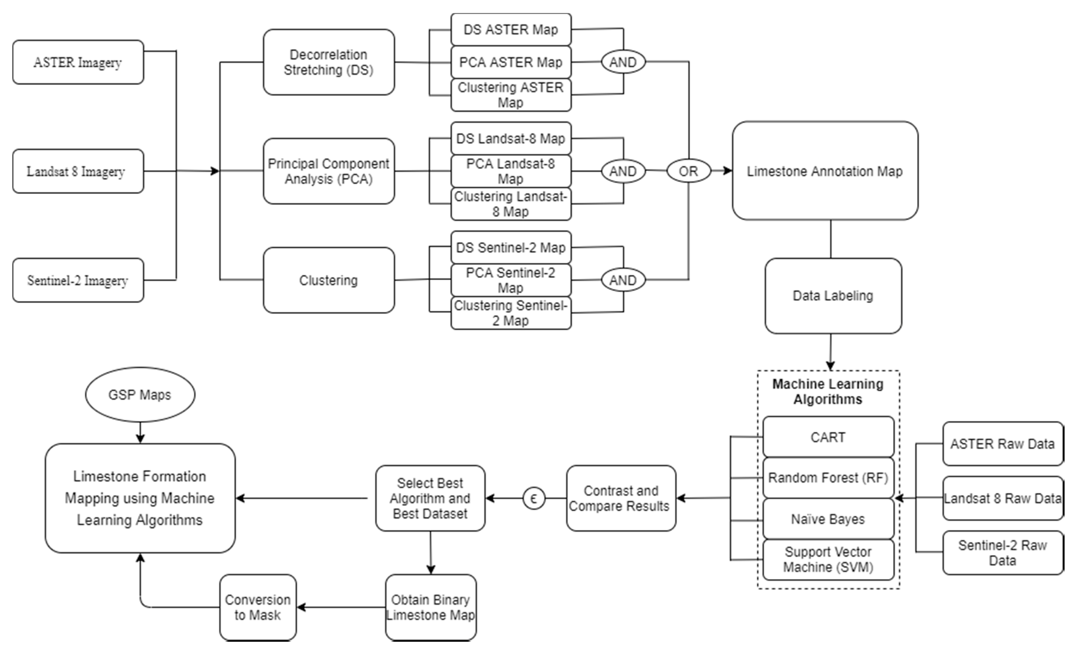
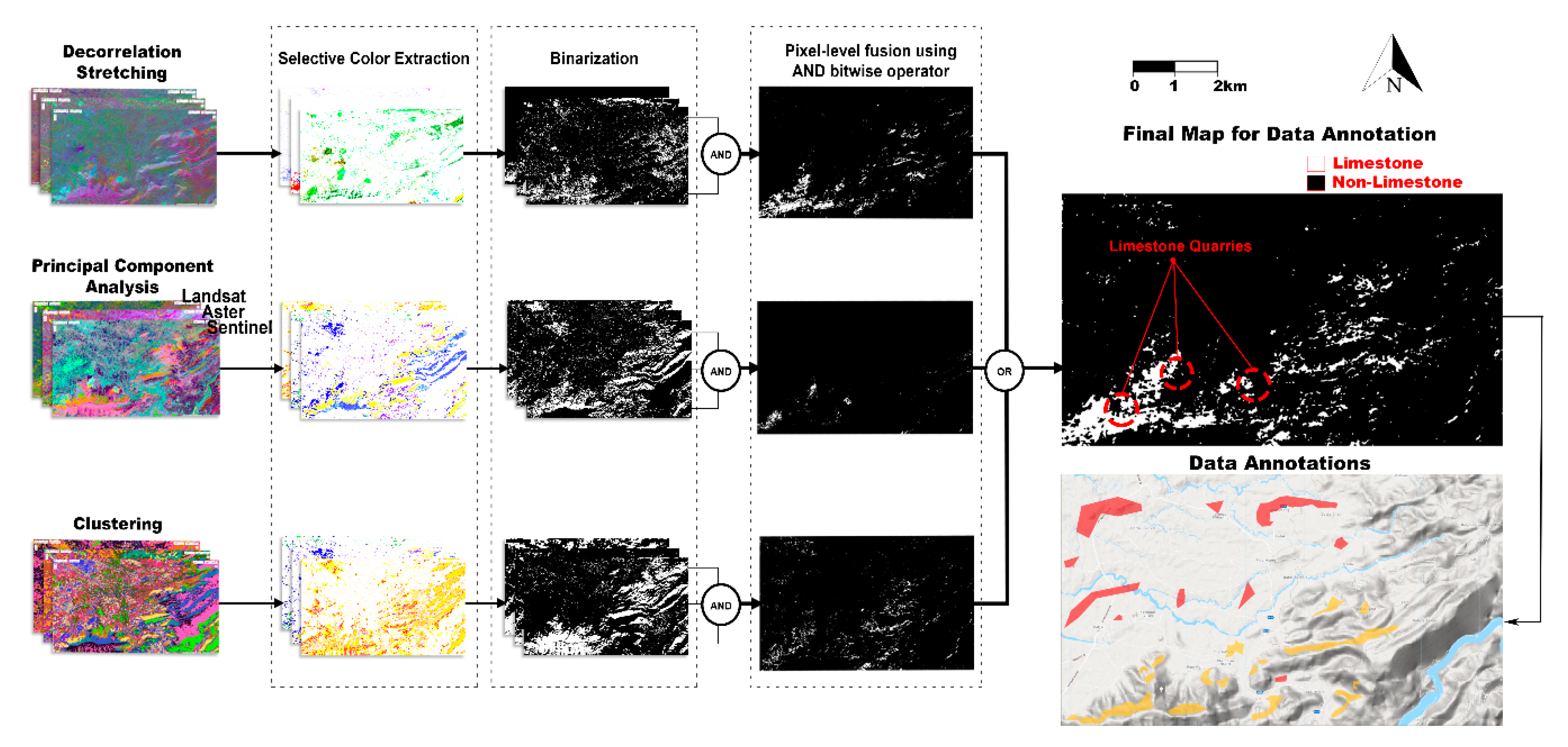
Initially, sample patches were taken from the GSP map to classify three lithotypes (i.e., two dominant allochemical types of limestone formations and Hazara slate and land covers) by applying four MLAs on three multispectral data sources using Google Earth Engine (GEE). Next, nine thematic maps were generated by applying PCA, DS, and X-means classification to ASTER, Sentinel-2, and Landsat-8 OLI. The three maps representing a common technique, but different data sources were fused with an AND operator, and the resultant three maps of each technique were fused with an OR operator to obtain the binary limestone labels. Selected patches from these labels were fed to CART, RF, NB, and SVM algorithms to perform binary limestone classification using the three data sources. Hyperparameters were explored to obtain better training results for limestone mapping. The maps obtained after applying different classifiers were validated by field visits along traverses (shown in
Figure 1) across the strata strike, where Global Positioning System (GPS) coordinates were recorded with photographs of the outcrops. The binary limestone classification map was used as a mask to further sub-classify oolitic (Samanasukh) and fossiliferous (Lockhart, Margalla) limestone formations. Training patches were selected from field surveys, and the data source with the highest reported accuracy for the binary limestone mapping was fed to CART, RF, NB, and SVM algorithms. The detailed methodology of the study is summarized in
Figure 2.
5.1. Multispectral Data Acquisition and Pre-Processing
Images were acquired using GEE with the least vegetation, cloud cover, noise, and shadows from the GEE database. No mosaicking was necessary, since, in GEE, strips of collected data are packaged into overlapping “scenes”, i.e., ASTER having a 60 × 60 km scene, Landsat-8 with 170 × 183 km, and Sentinel-2 with 290 × 290 km scenes were enough to cover the whole region. Data were selected for dry seasons to avoid vegetation; terrain, geometric, and radiometric corrections were also performed on the ASTER dataset. United States Geological Survey (USGS) Landsat-8 surface reflectance (SR) scenes were collected from the Collection 1 Tier 1 (T1) suite of Landsat-8 images, scaled and calibrated at the sensor level. Sentinel-2 level 2A corrected data were used with the bottom of atmosphere reflectance in cartographic geometry and atmospherically corrected using Sen2Cor processor and PlanetDEM. The scenes at different times were filtered with less than 5% cloud cover; a pixel-level median-based composite mosaic was used to obtain an image with the least vegetation, noise, and cloud cover where the median of each pixel in a band of the selected scenes was computed to compose the image for classification.
5.2. Limestone Formations and Hazara Formation Mapping
Initially, limestone allochemical formations, i.e., oolitic and fossiliferous, were mapped along with adjacent Hazara formation and other land covers (i.e., water, vegetation, fields, and buildings) by collecting training samples from the GSP Map 43C/9 and Hazara Map [
44] (please see
Figure 1), lying on either side of the region of interest, and MLAs such as SVM, NB, RF, and CART were applied to generate classification maps.
5.3. Fusion of DS, PCA, X-Mean Clustering Results for Limestone Annotation Map
To refine the training labels used in MLAs, ASTER, Sentinel-2, and Landsat-8 bands with established spectral sensitivity to limestone [
5,
7,
16,
17,
18,
19,
20,
21,
22,
23] were used to apply PCA, X-means clustering, and DS before fusion (please refer to
Table 1). Red-Green-Blue (RGB) based false color composite (FCC) images were made from the selected distinct components identified by the Crosta technique for the respective data sources, as shown in
Table 1. Each principal component was visualized as a single image; the three best components for each dataset, which distinctively highlighted the known limestone quarry locations in the image, were selected using the Crosta technique.
During the X-means classification, all the available bands within the data were used to obtain clusters with similar spectral responses for each data source. Similarly, DS was applied on each data source, and FCC of all possible combinations of stretched bands was compared with known limestone locations on the field to select the best ASTER, Sentinel-2, and Landsat-8 bands.
A set of nine thematic maps was obtained from three techniques, i.e., PCA, DS, and Clustering, applied to each of the three data sources. In each map, regions with known limestone occurrences representing the same color were extracted to grayscale and then binarized using a threshold of 245 for a maximum pixel intensity of 255. Three maps, each representing a particular technique, i.e., PCA, DS, and clustering, were obtained using bitwise AND operation on the three maps from each data source but the same unsupervised technique. The AND operator retains limestone regions, commonly identified by the thematic maps obtained from applying the same technique to all three data sources. This fusion ruled out many false positive limestone indications due to ANDing by eliminating limestone regions not indicated by applying a specific technique to all three datasets.
Further, the OR operator’s application allowed for the union of the three binary maps obtained after the AND operator, integrating limestone indications reported by any of these three techniques. These three maps were fused using an OR operation on binary limestone pixels to obtain a final map for data annotation. The resultant image’s noise was filtered out using a 5 × 5 median filter, and limestone annotations were refined using a morphology filter with a 5 × 5 square structuring element. The final image was used to select data annotations for use in supervised classifications representing the most probable limestone indications while applying three unsupervised techniques to three data sources.
5.4. Mapping Limestone Using Machine-Learning Algorithms
Geometric polygons that represented limestone and others, were selected as labels from the fusion map obtained from the PCA, DS, and X-means. Samples of each dataset inside the yellow (limestone) and red (non-limestone) polygons were selected and randomly split into a 70:30 ratio as training and testing pixels. The number of pixels varied for each data source, i.e., 31273/6702, 31377/6582, and 31530/6620 train/test split for Landsat-8, Sentinel-2, and ASTER, were used respectively. Once labels were obtained for training, Landsat-8, ASTER L1T, and Sentinel-2 MSI data was fed to the CART, SVM, naïve Bayes, and RF classifier to generate binary limestone maps. Since limestone shows distinguishable characteristics near the SWIR range [
5,
7,
16,
17,
18,
19,
20,
21,
22,
23], SWIR bands of ASTER, Sentinel-2, and Landsat-8 (as given in
Table 1) were used as input variables during training and validation of the ML algorithms for classification. The hyperparameters for all the four classifiers were tuned using grid search on a range of values chosen from the literature [
11,
61,
62,
63,
64], as indicated in
Table 2.
The overall (OA), user/consumer (CA), and producer (PA) accuracies were computed from the confusion matrix [
65]. The OA is the percent of the total correctly mapped pixels out of the range of pixels in the error matrix. CA is the complement of commission errors, and PA the complement of omission errors associated with each class/category [
65,
66,
67]. The Kappa coefficient measures the classification performance compared to randomly selected test values from the defined labels. It is an additional reliability metric, reporting corresponding values as −100 to 100% for worst to best classification results [
65,
68]. A Kappa coefficient value of 0 means that classification is no better than randomly assigned values.
5.5. Mapping Oolitic and Fossiliferous Limestone Formations in the Area
The resulting binary limestone map was used to obtain an image mask for the best data source reporting higher limestone accuracy. This enabled masking out non-limestone regions from the data, significantly reducing data mislabeling and misclassification of limestone formations. The region bounded by binary limestone classification map was used to discriminate Samanasuk (oolitic) and Margalla/Lockhart formations (fossiliferous) by application of CART, RF, NB, and SVM algorithms on the three data sources separately, using the best hyperparameters reported for binary limestone classification and validated by field observations.
6. Results and Discussion
The mean band spectra of limestone quarries and formations (Samanasuk, Lockhart, Margalla, Chorgali) against Hazara formation (slates), water, land, and vegetation are shown in
Figure 3. Limestone indicated signature reflection at 1.6 μm and absorption at 2.3 μm, in agreement with a previously conducted study [
11]. The mean band responses of slate can be easily distinguished from limestone formation spectra, indicating their spectral and compositional differences. Moreover, vegetation and land spectra were also in contrast to limestone and slate; thus, training/testing samples selected for limestone mapping were free from vegetation spectral signatures.
Initially, MLAs trained and validated approximately 2760 km
2 area using labels from GSP maps and field knowledge, while reporting 83.28% as the best overall accuracy (OA) by the RF algorithm (please refer to
Table 3). Further improvements in the results were investigated by obtaining data labels from the fusion of multi-source data after applying unsupervised techniques.
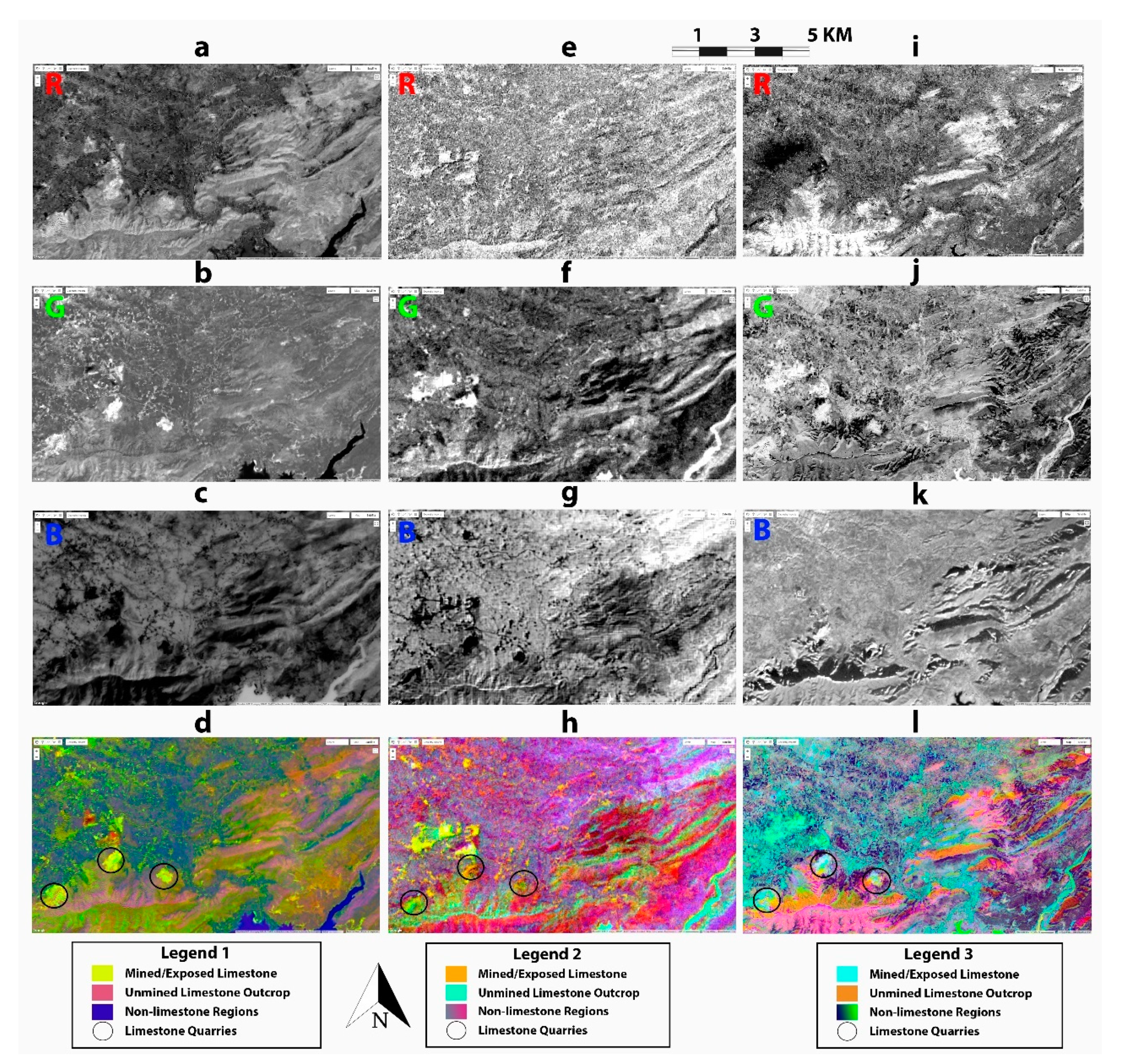
The results from PCA, X-means clustering, and DS applied on ASTER, Sentinel, and Landsat-8 datasets are presented in
Figure 4 and
Figure 5. Components retaining general information, i.e., vegetation and topography, were ignored (i.e., PC1, PC4, PC6 of Sentinel-2, PC1, PC3, PC6 of Landsat-8, and PC1, PC3, and PC5 of ASTER data). Components showing contrast in limestone were retained, i.e., PC6 and PC4 of ASTER showed limestone as bright due to positive loadings for SWIR8, TIR1, and TIR2 bands, while negative loadings of SWIR8 showed limestone as dark in PC2. Color composites of PC6, PC4, and PC2 shown in
Figure 4 indicated limestone quarries in light green and other limestone outcrops in turquoise green color. Similarly, PC5, PC4 of Landsat-8 and PC5, PC3 of Sentinel-2 indicated limestone as bright, whereas it was shown as dark in PC2 for both data sources. In both cases, SWIR2 was receptive to limestone, FCC of PC5, PC4, and PC2 of Landsat-8 highlighted limestone quarries in lime color and unmined limestone regions green and purple. Similarly, FCC of PC5, PC3, and PC2 of Sentinel-2 highlighted limestone quarries in white color with traces of turquoise blue shades (see
Figure 4). These spatial and spectral variations of colors represent variation within weathered limestone outcrops compared with freshly exposed limestone in cement quarries.
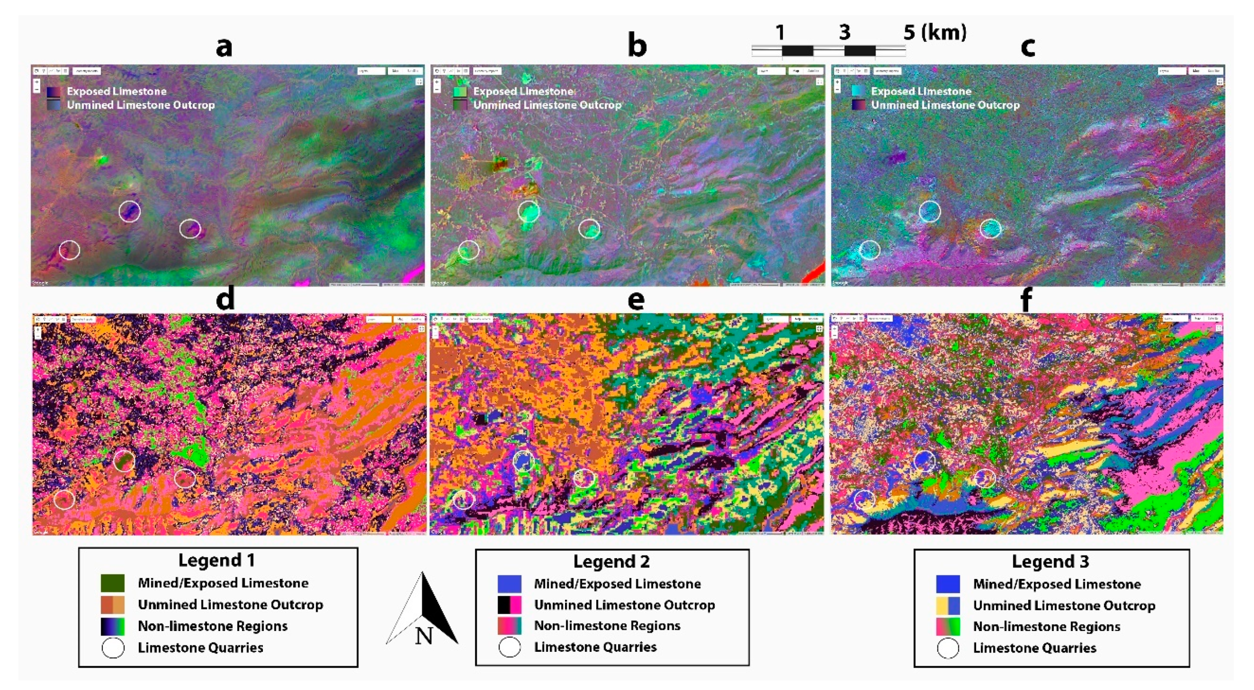
The results obtained using composites of Landsat-8, ASTER, and Sentinel stretched bands exposed the limestone region in navy blue, pale-green, and sky-blue colors, respectively (
Figure 5). The upper and lower limits of the range of clusters for the X-means clustering algorithm was set to 2 and 30, respectively. The optimum number of clusters for Landsat-8, ASTER, and Sentinel-2 were identified as 21, 19, and 20, respectively. Limestone quarries were highlighted as dark green for Landsat-8, blue for ASTER, and Sentinel-2 (
Figure 5). Surrounding limestone regions were golden-brown and pink for Landsat-8, pink and black for ASTER, and turquoise blue and cream in case of Sentinel-2 results, respectively (
Figure 5).
Sentinel-2 had the highest spatial resolution among the datasets, thus reporting the highest number of clusters. Due to the variations between different limestone formations, possibly due to weathering effects or noise, they were clustered into several classes, each with a different spectral mean. The three significant formations in the area, Samanasuk (Oolitic) and Lockhart/Margalla (fossiliferous) were shown by the clustering algorithm as teal blue, basil green, lapis blue, fuchsia pink, and banana yellow colors (
Figure 5f). This indicated distinctive spectral variations between these limestone formations; therefore, they were explored for further classification by more robust MLAs.
Limestone quarries of Dewan, Bestway Farooqia, and Bestway Hattar factories and limestone striking in the northeast/southwest direction were evident in all nine maps. The binary map obtained from the fusion of the nine maps shown in
Figure 4d,h,l) and
Figure 5 can be seen in
Figure 6, which shows limestone regions in white and non-limestone in black. All three limestone quarries were identified, along with some limestone regions in the surrounding area and the northeast and east of the Hazara formation. The binary limestone map from fusion contained many false negatives but insignificant false positives; therefore, reliable for limestone label selection from regions besides limestone quarries, improving the classification models’ generalizability.
Figure 6 also show the geometric polygons that represented limestone and others that were selected as labels from the fusion map obtained from the PCA, DS, and X-means to train the MLAs.
As shown in
Table 4, after feeding these refined labels for binary classification, CART presented the best accuracies (>90.00%) for all three datasets outperforming the random forest algorithm.
Table 4 shows the overall (OA), producer (PA), and user/consumer (CA) accuracies and Kappa coefficient (K) for the lithological classification using the CART, RF, NB, and SVM methods applied on Landsat-8, ASTER-L1T, and Sentinel-2 MSI datasets. One main reason could be that the composite had the least vegetation than other data sources. Due to better spatial resolution and a high level of vegetation, Sentinel-2 results were more detailed but had lower accuracy than Landsat-8. Therefore, while mapping allochemical limestone formations, the hyperparameters were tuned only for Landsat-8 data using the 6753 validation pixels, since it resulted in the best binary limestone classification accuracy.
Bachri et al. [
11] reported 96.08% CA for limestone class while mapping ten different lithologies, including limestone in Moroccan Anti-Atlas using 228 training pixels and 51 testing pixels by SVM with an RBF kernel, with the C and gamma parameters set as 100 and 0.16. Hyperparameters for different MLAs that reported the best corresponding accuracies during this study are given in
Table 5. In this case, the SVM reported 95.60% overall accuracy and 98.60% user accuracy for the polynomial kernel of degree 2, and the cost (C), gamma, and Coef0 of 2 × 10
−5, 0.471, and 10, respectively, while the voting and margin decision procedure produced the same results. Linear kernel reported the best overall accuracy of 94.13% for C=10 compared to 93.04% for Nu=0.2; therefore, C hyperparameter was used instead of Nu. Higher accuracy for C and Nu’s lower values indicated very subtle differences in spectral signatures, such as the weathered limestone around the cement quarries. The linear kernel accuracy fluctuated between 91.13 and 94.13% within the given range of C/Nu hyperparameters. The gamma parameter’s effect was not prominent on model accuracy; however, best results were mostly obtained for a gamma value of 0.471. The sigmoid and RBF kernels of the SVM and NB algorithm reported lower accuracy, while Landsat-8 and Sentinel-2 responded with better accuracy than ASTER data. CART application on Landsat-8 OLI data reported the best results with the corresponding OA and CA of 99.63 and 99.69% and Kappa coefficient of 0.99, respectively (as shown in
Table 4 and
Table 5). Random forest as an ensemble of decision trees did not perform well compared to CART, which may be due to better annotation of data by fusion of images from the application of unsupervised methods discussed earlier.
RF algorithm’s cross-validation accuracy decreased with the increase in the number of trees, while CART accuracy increased with the increase in “maximum number of nodes” until it reached 20; beyond this, no change was observed in the accuracy. Random forest resulted in higher accuracies for a higher value for “number of maximum nodes” (i.e., 100). Since CART outperformed RF, SVM, and naïve Bayes algorithms, only the CART classifier map was retained for allochemical classification of limestone.
Finally, the binary limestone classification map of 99.63% accuracy (
Figure 7A) was used as a base for the extraction of oolitic and fossiliferous limestone labels to map these limestone formations. Consequently, the Hazara formation (seen in
Figure 7B) was masked out before this classification, hence decreasing the chances of misclassification. After masking Landsat-8 composites, accuracy was improved for both RF and CART algorithms; however, RF had the highest OA accuracy, i.e., 96.36%, with respective CA of fossiliferous, oolitic limestone as 97.49 and 94.64%, as given in
Table 6 and
Figure 7C. The limestone formation classification map validated the formation strike, i.e., in the northeast–southwest direction, in line with the field observations and published literature [
69].
Therefore, the results suggest that limestone allochemical classification improved when the classification was performed in a limestone-only region obtained through masking Landsat-8 composite with CART binary classification map. The resultant classification was more reliable than the earlier case when the RF algorithm reported an overall accuracy of 83.28%, referred to in
Table 3.
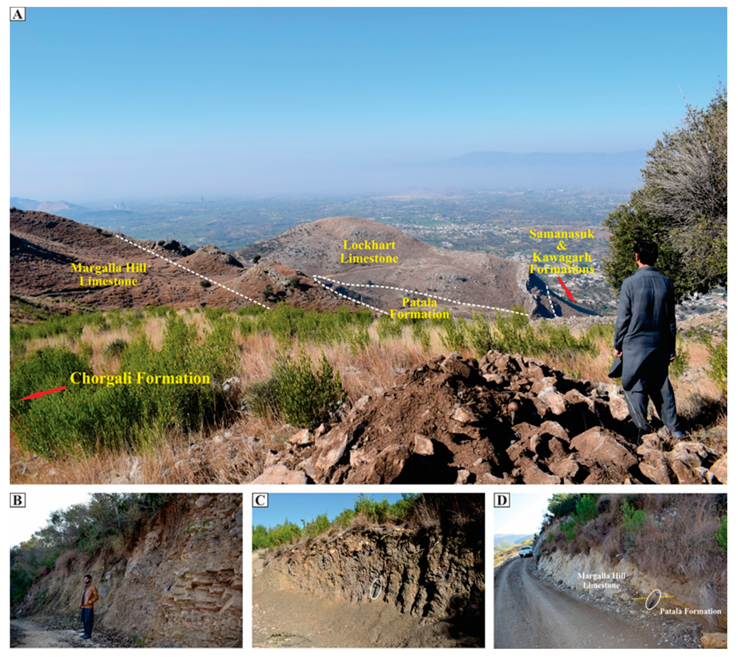
Field visits (shown in
Figure 8) performed along the traverse shown in
Figure 1 validated the binary limestone map reported by application of CART algorithm on Landsat-8. Several limestone-bearing formations with predominantly limestone lithology (i.e., Samana Suk formation, Lockhart and Margalla Hill limestones) and those with limestone and interbedded shale (i.e., Kawagarh, Patala, and Chorgali formations) were differentiated.

 ,
, 


