Multi-Temporal Time-Dependent Terrain Visualization through Localized Spatial Correspondence Parameterization

Abstract

Visualizing quantitative time-dependent changes in the topography requires relying on a series of discrete given multi-temporal topographic datasets that were acquired on a given time-line. The reality of physical phenomenon occurring during the acquisition times is complex when trying to mutually model the datasets; thus, different levels of spatial inter-relations and geometric inconsistencies among the datasets exist. Any straight forward simulation will result in a truncated, ill-correct and un-smooth visualization. A desired quantitative and qualitative modelling is presumed to describe morphologic changes that occurred, so it can be utilized to carry out more precise and true-to-nature visualization tasks, while trying to best describe the reality transition as it occurred. This research paper suggests adopting a fully automatic hierarchical modelling mechanism, hence implementing several levels of spatial correspondence between the topographic datasets. This quantification is then utilized for the datasets morphing and blending tasks required for intermediate scene visualization. The establishment of a digital model that stores the local spatial transformation parameterization correspondences between the topographic datasets is realized. Along with designated interpolation concepts, this complete process ensures that the visualized transition from one topographic dataset to the other via the quantified correspondences is smooth and continuous, while maintaining morphological and topological relations.

1. Introduction

Time-dependent visualization of changes in physical entities, such as topographic datasets that present morphologic alterations, requires mutually modelling a series of discrete given datasets. The presumption is that these topographic datasets, such as Digital Terrain Models (DTMs), were acquired on a given time-line and that they represent approximately the same coverage area. An infinite set of topographic datasets, which present a time interval of close to zero (t→0), is practically not realistic. The reality of physical phenomenon occurring during acquisition times together with existing geometric and morphologic ambiguities add to modelling the complexity of the observed datasets. These factors will certainly contribute to the existence of different levels of inter-relations and geometric inconsistencies among the topographic datasets. The commonly used “flip-page” animation method, for example, where each terrain model serves as key-frame (or key-phase), will not suffice [1]. This is mainly due to the fact that the different topographic datasets are non-rigid objects; thus, they are quite different from one another, i.e., store different geometric structures and characteristics (differences in level-of-detail and resolution, datum ambiguity, global and local discrepancies—to name a few). Any straight forward simulation that ignores preliminary mutual registration and modelling that takes into consideration these factors will evidently result in an un-realistic representation and sometimes truncated, ill-correct with “topographic artifacts” and un-smooth simulation. Figure 1 depicts such an example, where two topographic datasets represent the same morphologic entity (a hill in this case)—but each with different position in respect to the same reference system (left). A straight-forward simulation will present an ill-correct result, where the same entity is presented twice during transition (middle); the correct transition must take under consideration that spatial relations exist (e.g., inconsistencies) between the two—in this case, displacement in the x-axis—before any simulation can take place (right), thus presenting only a single entity that exists in reality.

Figure 1. Two topographic datasets representing the same morphologic entity with different positions (top-left and bottom-left), an ill-correct straight-forward transition (middle) and desired transition (right).

Figure 1. Two topographic datasets representing the same morphologic entity with different positions (top-left and bottom-left), an ill-correct straight-forward transition (middle) and desired transition (right).

Understanding and modelling the complex inter-relations that exists between topographic datasets is therefore essential. This paper introduces a novel hierarchical modelling algorithm that establishes a quantitative mutual modelling via sets of spatial correspondences that best describes the morphologic changes occurred; thus, it enables us to carry out more precise, true-to-nature and realistic animation visualization and simulation tasks. These are essential for a reliable 3D Geographic Information Systems (GIS) workflow, while trying to best describe and simulate the reality transition as it occurred.

When considering geospatial GIS work environments, the basic requirement is that it enables support of different types of data-models, i.e., representations and structures, while enabling—if required—on-the-fly simulation of specific objects representation. Several aspects can be mentioned as basic requirements [2], while others are derived expressly when dealing with terrain and multi-temporal representations:

• Modelling complexity—the topographic reality that is based on 3D physical objects is normally very complex: geometric and semantic information—to name a few;
• Multi-resolution and multi-representation—when dealing with multi-epoch and multi-source terrain representation the physical objects representing terrain are rarely of the same nature;
• Presentation and appearance—usually when representing 3D terrain data the viewer will demand the representation to be as true-to-nature as possible and not derived by data symbols and annotation;
• Animation—terrain animation has to preserve the quality and accuracy of given data, as well as be realistic and continuous throughout the simulation;
• Simulations and multi-temporal representations—chosen algorithm needs to handle the general problem of physical objects (or skeletons) derived deformation instead of treating each area of anatomy as a special case;
• Topologies and morphologies—are to be preserved or otherwise created if derived by the deformation process, while maintaining the realistic nature of representation.

Techniques and methods, which involve the transformation of one object to another object (e.g., topographic entities), while creating a continuous transition of shape sequences that changes gradually, are being developed in recent decades on many aspects in the field of computer graphics (e.g., [3,4]). These techniques, which are best known within the terminology of shape morphing and shape blending, attempt to create a natural visual effect and are used mostly for various animation tasks in television and movies. The transformation process is usually expressed (visually) by the geometry of the source and destination objects. The main challenge is establishing algorithms that will be able to match spatially the objects that are different from one another. This has to be achieved with minimal user intervention, while maintaining the properties of objects to maximum extent possible [5]. It is obvious, then, that achieving this challenge and the abovementioned criteria is intensified when dealing with the complexities of topographic representations required for real (virtual-reality) GIS and mapping applications, such as morphologic alterations simulations.

2. Related Work

Methods of substitution between objects, i.e., transformation solutions, mainly deal with the problem of correspondence between physical objects. The transformation that is mostly performed is a linear substitution between objects. This is usually carried out for basic-primitives sequence alignment, but still sometimes leads to well-known 3D object artefacts, such as “collapsing joints” and the “candy wrapper” effect [6]. These artefacts are normally caused when a linear blending is implemented while the rotation matrices involved have a large angle between them. Respectively, such a solution might produce transition that is ill-defined and not visually natural and realistic. Intuitively, the transformation process should strive to transform objects as rigidly as possible, while avoiding local distortions by utilizing complex solutions rather than a clear linear substitution, such as the commonly used “flip-page” mechanism. This technique does not try to attempt solving mutual existing relations, but rather only to produce an abstract and simplified simulation and representation, while the result will present topographic artifacts. Examples are depicted in Figure 2.

Figure 2. Animated topography via linear “flip-page” transition showing artificial morphologic entities: cliff (left) and ravine (right).

Figure 2. Animated topography via linear “flip-page” transition showing artificial morphologic entities: cliff (left) and ravine (right).

Procedures, such as shape blending or shape morphing, utilize a process in which one object is combined with another object, while trying to stretch, rotate and move it in order to create a maximum matching between the two objects. Two major problems or tasks have to be addressed for this assignment [7]:

• Vertex Correspondence, i.e., figuring out which vertex in one object should blend with another vertex in the other object; this can be defined in the problem at hand as spatial correspondence, i.e., which entity (and parts of entity) in one topographic dataset corresponds to another entity in the other topographic dataset, while the correspondence is modelled and quantified by transformation parameters. A trivial solution to this is to leave it to the animator himself to decide, i.e., manual sampling of selection of points, which will define the connectivity between both physical objects, thus finding their mutual coordinates connectivity.
• Vertex Path (trajectory problem), i.e., figuring out what path the vertices should take to get from one object space to the other. This problem can be resolved only after the vertex correspondence problem is solved. This problem stems from the question of how to transform the source object points to the destination object points. The trivial solution for this is the substitution of linear transformation between the points. As stated earlier, this is not usually the preferred natural and realistic solution, so more complex solutions are required to solve this, such as, including distortions and squinting in the intermediate objects to maintain natural visualization (e.g., [8,9]).

These problems are relatively straightforward to solve in the case of spatial rigid body models, such as a face, which mainly differ in their perspective point of view (e.g., [10,11,12]). The fact that the two given rigid models acquired at different time epochs actually represent (or resemble) the same physical object contributes to less ambiguity and more robustness and certainty in carrying out the two tasks mentioned before. The number of points representing the two objects is also usually the same—as is the resolution. A problem arises when trying to solve this on topographic non-rigid geo-spatial datasets that represent reality, but might be quite different from one another, thus adding ambiguity to the vertex correspondence problem. Without executing this task, the vertex path will not produce adequate and realistic results.

Existing concepts and techniques aim at morphing one shape into another shape by concentrating on the shape itself, i.e., trying to stretch, compress and bend one shape into another shape over a given time period and in a realistic fashion (e.g., [13,14,15]). These works are not designed for the geographic information (GI) and mapping scientific fields, but rather to real-time virtual reality and animation in general. The study of [3], for example, led to the statement of the path-transition paradigm, which is a general methodology for creating 3D real-time color animations. This paradigm relies on the use of four abstract data types: location, image, path and transition. Still, it is based solely on 3D primitives, such as cones, spheres, cubes and others, as opposed to generality, where no geometric primitives’ a priori consideration can be made.

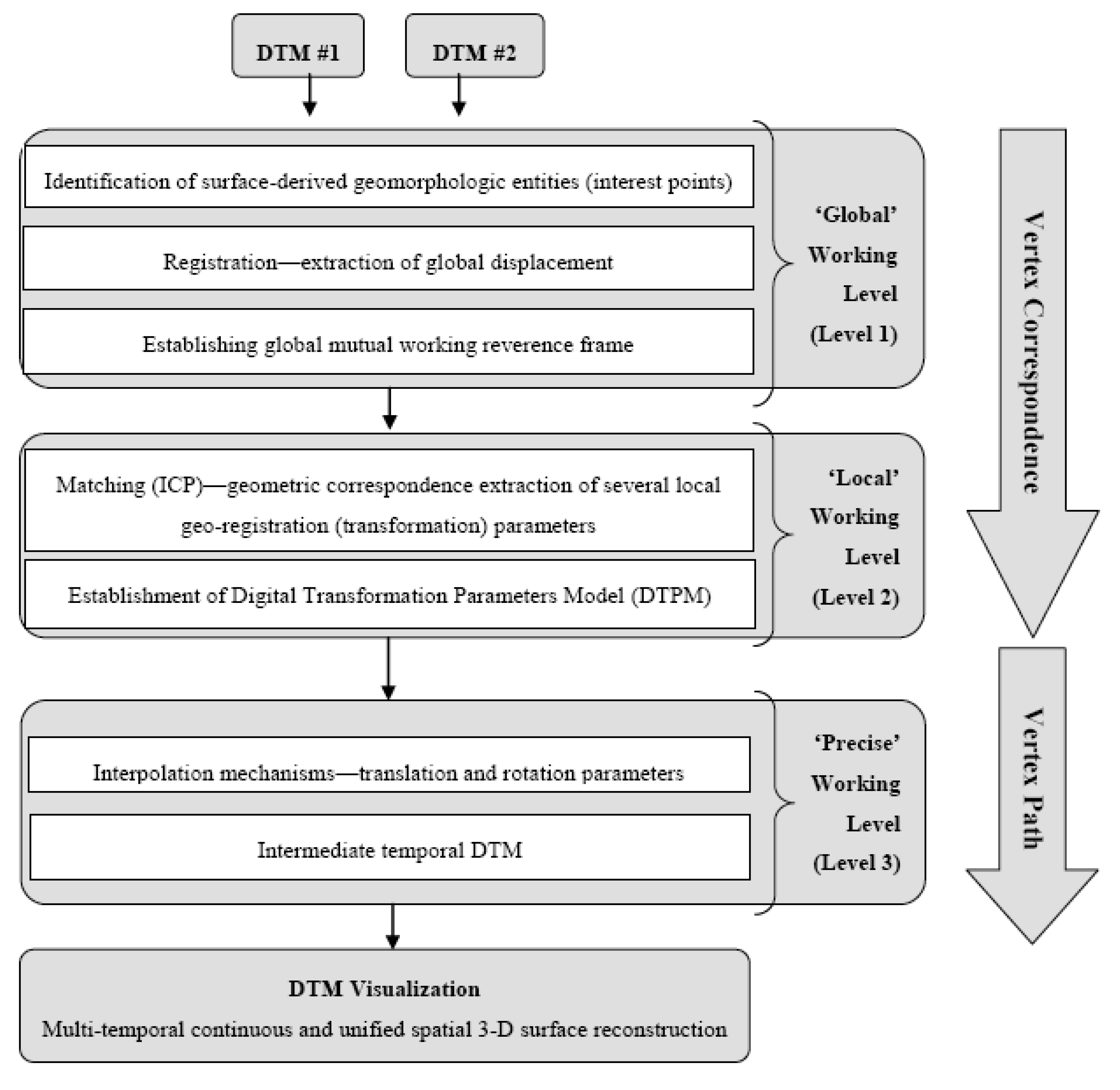
3. Proposed Approach

Hierarchical modelling designed for integration of two (or more) homogenous DTMs was proposed in the work of [16]. This mechanism exploits complete and accurate sets of different-scale data-relations and correspondence that exist within two DTMs that share a mutual coverage area. The division of the topographic datasets into several separate homogeneous hierarchical zone-levels, depicted in Figure 3, enables us to correctly define the correct localized spatial relations, such that the global and local geometric discrepancies are monitored and modelled before performing the actual integration process. This mechanism yields the establishment of a model that stores the local transformation parameterization between the topographic datasets, i.e., complete spatial correspondences expressed via translation and rotation parameters. The use of these data-relations enables the precise modelling of the DTMs, i.e., extracting a mutual reference working frame (schema) for data integration.

Figure 3. Hierarchical modelling schema, depicting three-working levels: global (registration, level 1), local (matching, level 2) and precise position-derived data-integration and interpolation (level 3).

Figure 3. Hierarchical modelling schema, depicting three-working levels: global (registration, level 1), local (matching, level 2) and precise position-derived data-integration and interpolation (level 3).

Figure 4. Workflow of the hierarchical modelling mechanism and its main stages. DTM, Digital Terrain Models.

Figure 4. Workflow of the hierarchical modelling mechanism and its main stages. DTM, Digital Terrain Models.

A short review of this mechanism and its main stages is given and depicted in the workflow in Figure 4. In general, stages 1 and 2 are designed to extract the local and precise vertex correspondence, while stage 3 is designed for the vertex path:

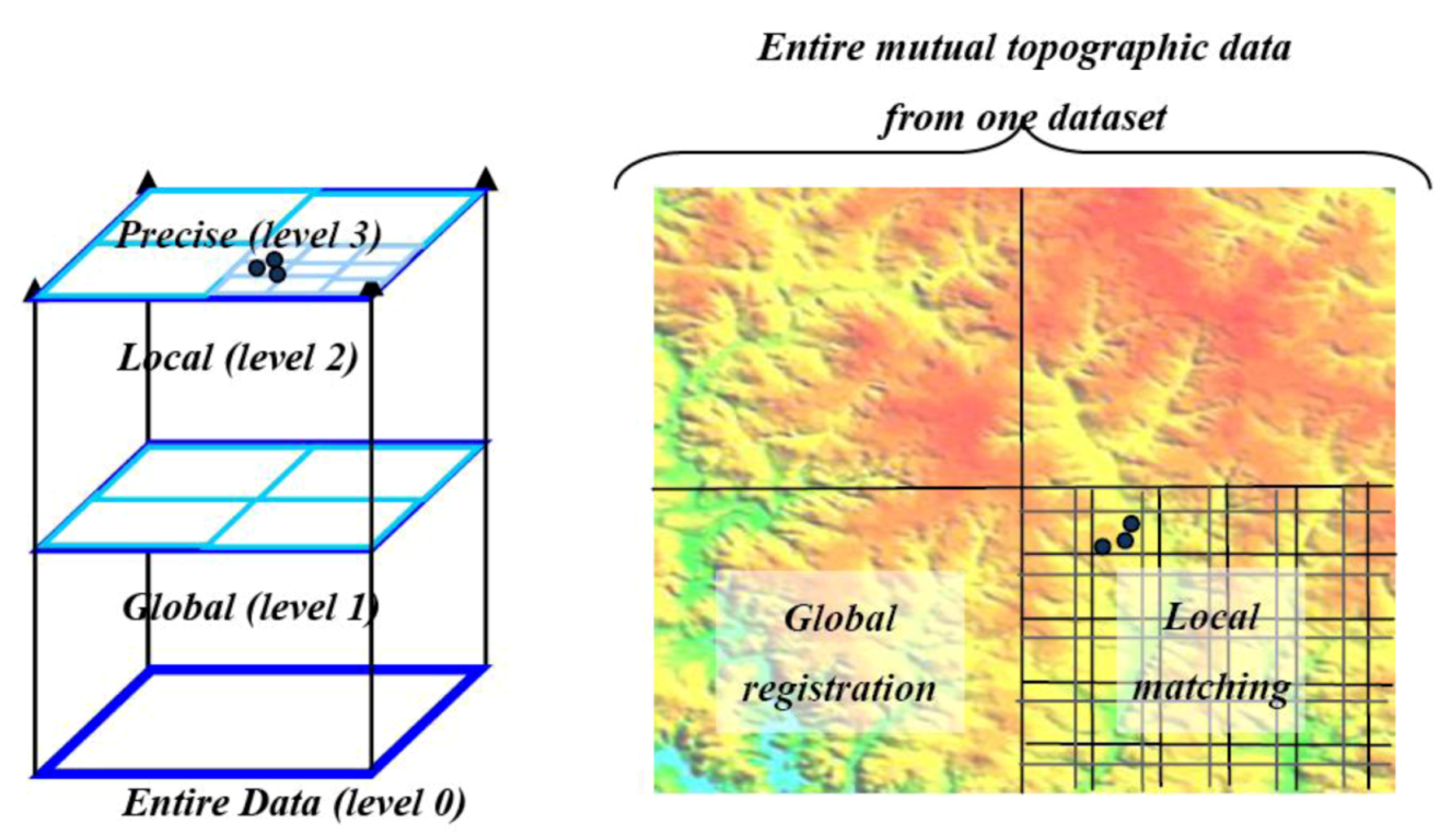
• Global rough registration, whereas choosing a common framework for both DTMs (and, thus, solving the datum and coordinate system ambiguities existing between DTMs before performing transformation, as outlined in Figure 1). This is achieved while implementing the Hausdorff distance algorithm that registers sets of selective unique homologous entities (objects) existing in both topographies’ skeleton structure. The skeleton structure of each DTM is identified via a novel topographical maxima interest point identification algorithm;
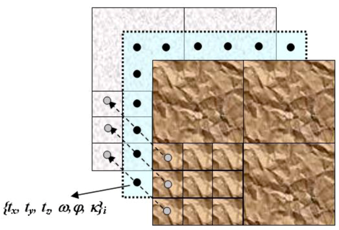
• Matching—since global registration is achieved and datum ambiguities are resolved, local matching is carried out while implementing the Iterative Closest Point (ICP) algorithm for rigid surfaces matching. This stage is essential for achieving precise reciprocal modelling framework between the two datasets, thus establishing localized transformation quantification;
• Integration schema, which consists of the modelling inter-relations quantification evaluated in the local matching. Since transformation is extracted via ICP on a local level, this quantification is needed to be densified for all points existing in that level, i.e., extracting transformation values for each DTM point independently to be transformed from one topographic dataset to the other. This densification is carried out via designated interpolation mechanisms, which are further developed to suit the task at hand (discussed in Section 4.2).

3.1. Correspondences Extraction

This stage encapsulates the processes associated with the hierarchical modelling of level 1 and level 2, which are designed to extract varied-scale data-relations and correlations in an automatic manner, i.e., all vertices correspondences exist between DTM #1 to DTM #2; this is vital parameterization required to create reliable visualization. This is carried out by registering—subsequently and independently—different area levels. In cases that the coverage area is extremely large, a level 0 can be considered, which takes the entire area and divides it to several level 1 areas. Based on the assumption that wide coverage topographic datasets present a resolution of 20–50 m, the volume of data needed to be analyzed derive the coverage areas. As such, the coverage areas used in the different analysis tasks are: level 1—100 km² (approximately 150,000 points for interest point identification); level 2—1 km² (approximately 2,000 points in the ICP process); and level 3—resolution (point) level.

Each area (j) of level 2, which is a result of a specific ICP process, can be represented by a set of local transformation quantification (in this case, an affine transformation used: three translation and three rotation coefficients—{t_xj,t_yj,t_zj,φ_j,κ_j,ω_j}. Structuring all the local transformation sets, one can consider this as a Digital Transformation Parameters Model (DTPM), depicted in Figure 5. This DTPM stores a series of vertex correspondences from a specific area in DTM #1 to its corresponding area in DTM #2; thus, yielding the idea in level 3—namely, vertex path. The fact is that the DTPM matrix is geo-referenced, while parameter values stored in the DTPM maintain continuity and smoothness within the entire coverage area. Hence, one can interpolate on these parameters to assess the precise required transformation, i.e., vertex path, for each DTM point to create a continuous transition between the different DTMs. Still, specific and explicit interpolation concepts that will maintain the different transformation behavior of the different parameters are required.

Figure 5. Digital Transformation Parameters Model (DTPM) transformation matrix (middle turquoise); and source and target DTMs (front and background). Each matrix cell (j) stores a local six-parameter transformation set.

Figure 5. Digital Transformation Parameters Model (DTPM) transformation matrix (middle turquoise); and source and target DTMs (front and background). Each matrix cell (j) stores a local six-parameter transformation set.

3.2. Path Evaluation

Hypothetically, when transforming a DTM grid-point from the source topographic dataset, while using the stored transformation parameters, should coincide with the terrain presented by the target topographic dataset. The (vertex) path from source to target is actually a hypothetical transformation between the two given physical objects that can be regarded as a time-dependent one, and any intermediate scene on that path is basically unique temporal terrain visualization.

Still, the resolution of the DTPM matrix is significantly lower than the given resolution(s) of the modeled topographic datasets. Usually, the topographic datasets used store grid-points in a resolution of a few meters up to several dozen. The DTPM resolution, however, is derived from the frame size used in the ICP matching process; thus, storing the parameters in a resolution of several hundred meters (e.g., 1 km²). The fact that position-derived unique transformation values are required for each point that exists in one topographic dataset (source) for transformation to the other topographic dataset (target), i.e., vertex path, yields that an interpolation on these values is required. Due to the discrete cell matrix’s structure, moving between neighboring cells, i.e., between different sets of six transformation parameters, might introduce value changes. Consequently, not implementing any interpolation on these values might produce discontinuities in the generated intermediate topography—discontinuities that will coincide to the DTPM cell borderlines.

Two interpolation procedures can be pointed out:

• Among the DTPM matrix’s grid-nodes (space-domain) to maintain continuity, while moving among cells. This computation is designated for the calculation of position-derived six parameter transformation values. These values are required to transform a grid-point that exists in the source dataset to its corresponding position in the target dataset;
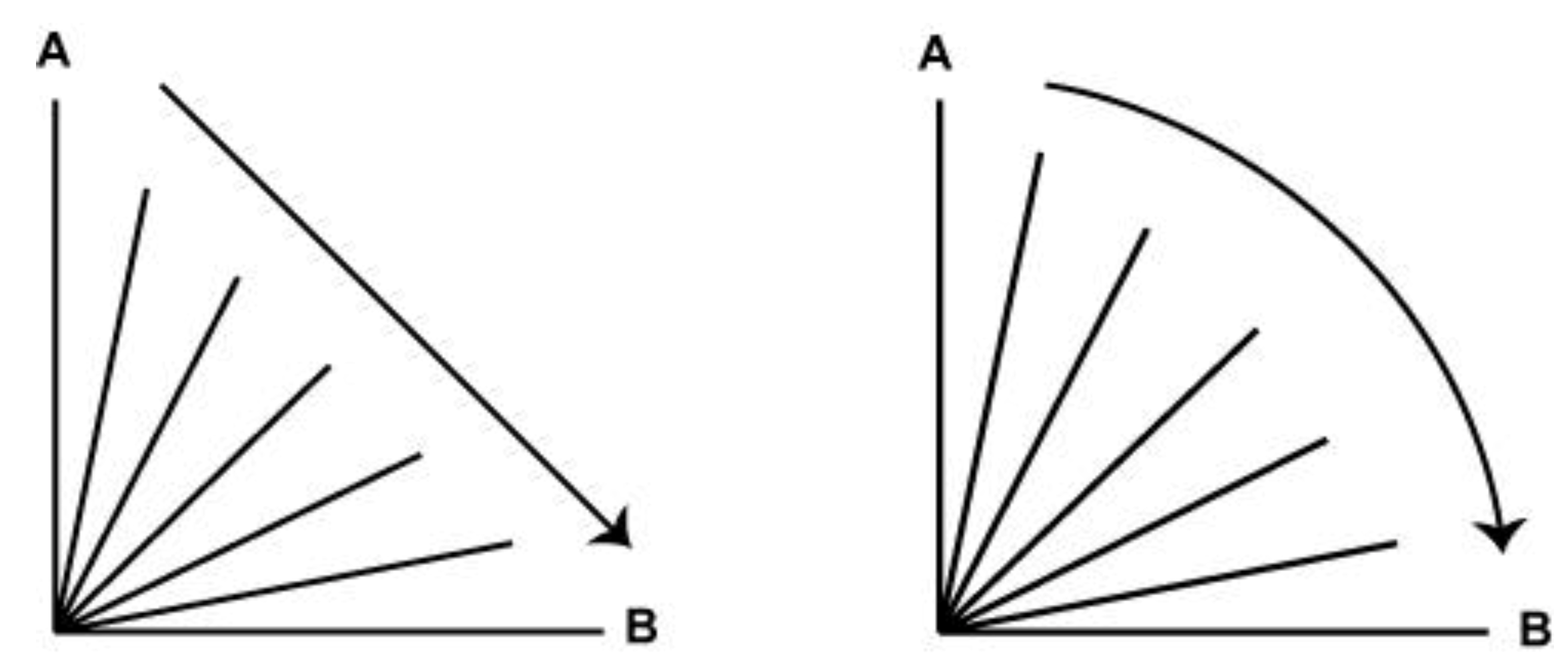
• In-between the topographic datasets/DTMs (time-domain). Spatially, it can be depicted as if the intermediate topography is situated in the space between the source and target topographies. The position of the intermediate topographic dataset is defined by the time-proportion and the magnitude of the transformations involved in the process.

Consequently, after the implementation of the “among” interpolation, an “in-between” interpolation is carried out on the values to appreciate spatially the position of the intermediate terrain within that space. The “in-between” (or path) interpolation is designed for the calculation of weighted six parameter transformation values from source topography (time = 0) to target one (time = 1), while time ∈ [0,1]. Each transformation value gradually varies from zero on the source topography, to its maximum value on the target one (that was calculated via the ICP process). Due to different data characterization of translation parameters and rotation ones, the suggested interpolation procedures are divided.

The next section presents the algorithms and the computational concepts designed for multi-temporal visualization that were implemented and integrated. Section 4.1 outlines the extraction of the vertex correspondence via the hierarchical registration process; this will include an explanation of algorithmic considerations and mathematical concepts required. Section 4.2 outlines the vertex path problem that is engaged via specific interpolation mechanisms.

4. Algorithm Outline

4.1. Local Matching (Vertex Correspondence)

4.1.1. General

The entire modelled area is divided into frames. Each congruent frame—one of each terrain representation—is matched via the ICP algorithm independently and separately. This localized implementation is more effective in monitoring and modelling local random incongruities, and trends exists. Thus, the estimation of the rigid body transformation(s) that aligns both models best is attained. This quantification is later used for the transformation—and deformation—of one object to the other.

ICP matching is accomplished via the minimization of a goal function based on least squares matching (LSM). This process measures the squares sum of the spatial Euclidean distances or errors, existing between geometries presented by congruent frames: g and f. The process output enables extracting the correspondence, expressed via the spatial transformation model, existing between the frames.

In order to perform least squares estimation, i.e., linearization, only the linear terms are retained (second and higher orders are omitted from the Taylor series). Consequently, each observation formula is related to a linear combination of the transformation parameters, which basically are variables of a deterministic unknown [17]. The 3D rigid body transformation model used here is composed of six parameters: three translations {t_x,t_y,t_z} and three rotations {ω,φ,κ}. The LSM model is written as a matrix notation in Equation (1):

(1)

where A is the design matrix (derivatives of the six unknown parameters), X is the unknown 6-parameter vector {t_x,t_y,t_z,ω,φ,κ}^T and l is the discrepancy vector that is the Euclidean distance between the corresponding DTMs’ frames (normally, DTMs represent reality in true scale; thus, it is assumed here that both datasets represent the terrain relief with approximately same scale factor (m), i.e., it is fixed to unity).

The least squares solution produces as the generalized Gauss-Markov model the unbiased minimum variance estimation for the parameters, depicted in Equation (2):

(2)

where X denotes the solution vector, v denotes the residuals vector of frame observations, σ₀² denotes the variance factor, n denotes the number of observations and u denotes the number of (unknown) transformation parameters, i.e., u = 6.

4.1.2. Non-Rigid Bodies Constraints

Due to the fact that both DTMs are non-rigid physical bodies, several aspects are considered:

• Wide-coverage DTMs represent different data-characteristics—namely, level-of-detail and resolution—implying that existing ICP homologous points is not at all explicit;
• DTMs acquired on different times (epochs) will surely represent different terrain topography and morphology (either natural or artificial activities);
• Data and measurement errors can reflect on the points’ positional certainty on a relatively large scale.

Addressing the aforementioned yields three geometric point-to-cell constraints that are implemented in the ICP process:

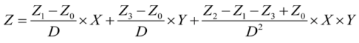
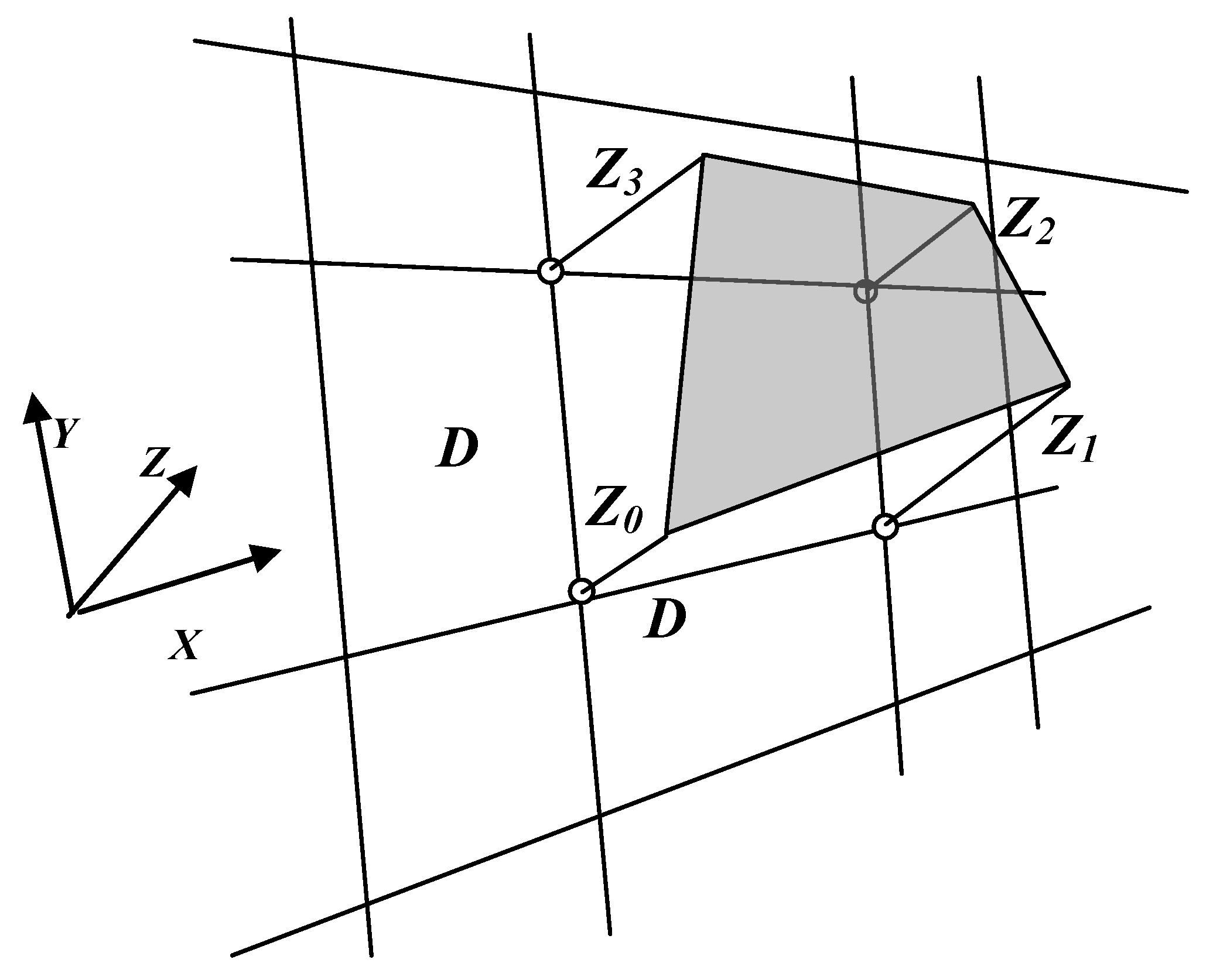
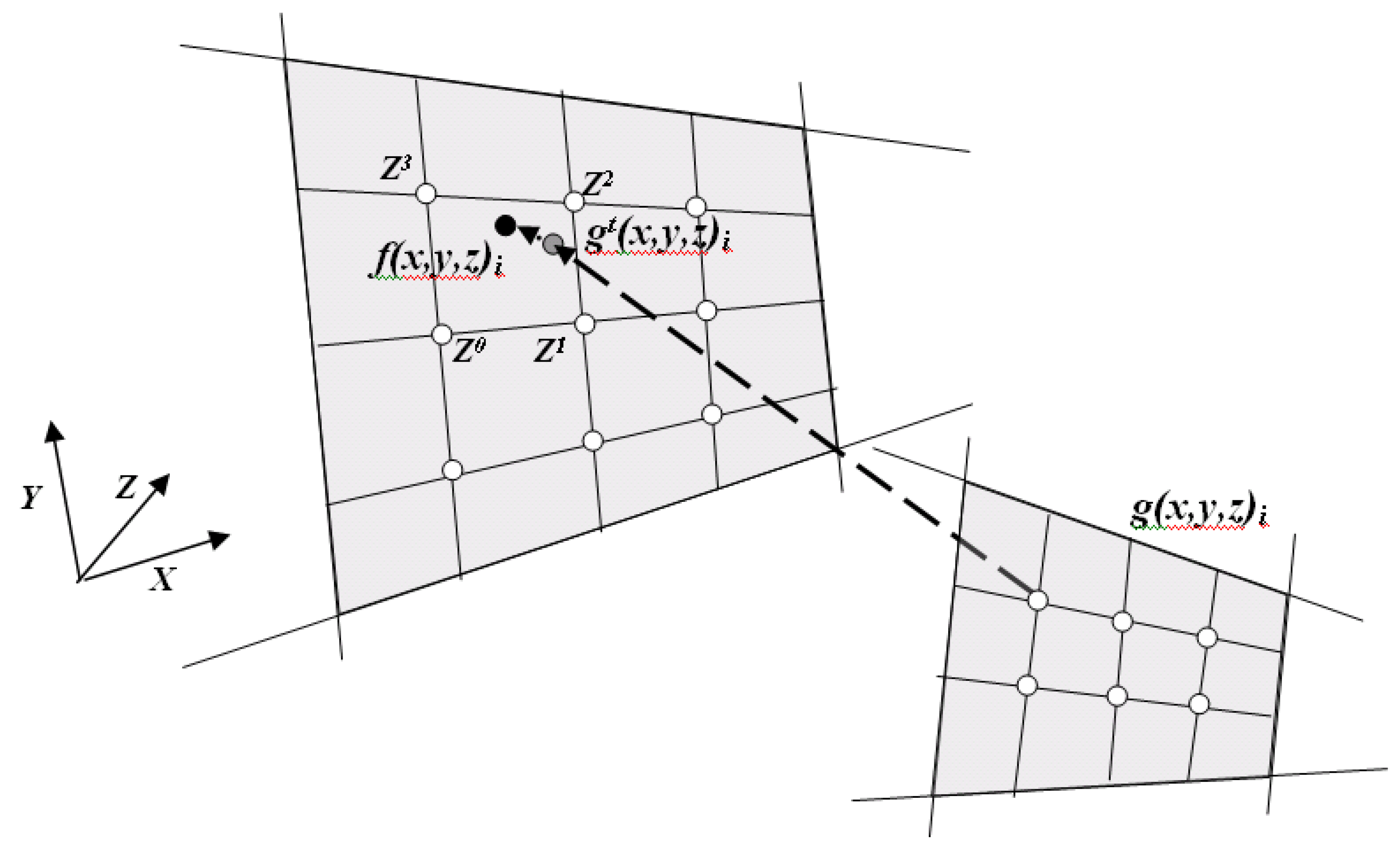
• The corresponding coordinates of the paired-up nearest neighbor i {f(x,y,z)_i} fit geometrically to a local cell-plane in frame f. Cell-plane geometry is defined here by a localized bi-linear interpolation: z(x,y) = a₀+ a × x + a₂ × y + a₃ × x × y, which is probably the most common way to calculate heights within a bounded rectangular grid-cell. The four coefficients {a₀,a₁,a₂,a₃} are calculated based on the cell’s corner heights, depicted in Equation (3) and Figure 6 (In cases where the triangulated irregular network (TIN) structure of topographic datasets is used, slight modifications of these equations are required to fit TIN’s triangular-plane characteristics. Still, though this data-structure is becoming, nowadays, more commonly used, mainly for data acquired by airborne laser scanning (ALS) technology, most of existing wide coverage DTMs are still stored and analyzed as a raster structure; thus, this will not be addressed here);
• The line-equation, derived from the coordinates of point i transformed from frame g (denoted by g^t(x,y,z)_i, where t stands for transformed) to frame f with the best known transformation parameters and the paired-up nearest neighbor, i, in frame, f {f(x,y,z)_i}, is perpendicular to the local cell-plane in frame, f, in the X direction (achieved by the first order derivative). This constraint validates that counterpart points, g^t(x,y,z)_i and f(x,y,z)_i, are the closest ones existing based on the shortest Euclidian distance;
• The same constraint outlined in 2 is applied, only here, the line-equation is perpendicular to the local cell-plane in frame f in the Y direction:

  (3)

where Z_i {i ∈ [0–3]} denotes the local DTM grid-cell corner heights, depicted in Figure 6, and D denotes the DTM resolution (slight modifications are required if different resolution values exist in both the DTM axis/directions).

Figure 6. Schematic indexing of local DTM grid-cell corner heights: Z_i {i ∈ [0–3]}.

Figure 6. Schematic indexing of local DTM grid-cell corner heights: Z_i {i ∈ [0–3]}.

The point transformed from g with best available transformation parameters (updated iteration) is defined by g^t(x,y,z)_i, while the counterpart point that in reality upholds the local plane cell is defined by f(x,y,z)_i. f(x,y,z)_i, which is the closest point, which exists to g^t(x,y,z)_i, has to validate the three constraints detailed earlier.

The first constraint for point f(x,y,z)_i is defined by Equation (4):

(4)

The second and third constraints enforce a closest point by requiring the first order derivative of the plane and the line connecting the two points (Equation (5)) to be perpendicular, i.e., multiplication equals the value of minus one (−1), depicted in Equation (6). The schematic explanation of the constraint process is depicted in Figure 5, where Z_i {i ∈ [0–3]} depicts the four grid-cell corners containing the closest point.

(5)

(6)

Thus, the last two constraints can be written as in Equation (7):

(7)

It can be described as if these criteria of constraints shift the vector between the points, g^t(x,y,z)_i (dark-grey) and f(x,y,z)_i (black), over the local grid-cell plane towards its final position, thus minimizing the least squares target function until converging to the final positioning of f(x,y,z)_i, depicted in Figure 7.

Figure 7. Schematic explanation of least squares target function minimization via three constraints: g^t(x,y,z)_i depicts the transformed point from g and f(x,y,z)_i depicts the counterpart point upholding the local plane grid-cell that is closest to g^t(x,y,z)_i.

Figure 7. Schematic explanation of least squares target function minimization via three constraints: g^t(x,y,z)_i depicts the transformed point from g and f(x,y,z)_i depicts the counterpart point upholding the local plane grid-cell that is closest to g^t(x,y,z)_i.

Summing up all (x,y,z) values of points from g and counterpart points from f within a specific frame yields (via the ICP process) the unified transformation quantification expressed by six parameters. These are stored in the DTPM, depicted earlier in Figure 5. As a result, the outcome of running this process is the precise quantification of all frame correspondences between the different topographic datasets. Still, a more localized precise quantification is required per grid-point and, also, the evaluation of the actual vertex path—both outlined in the next section.

4.2. Spatial Correspondence Parameterization (Vertex Path)

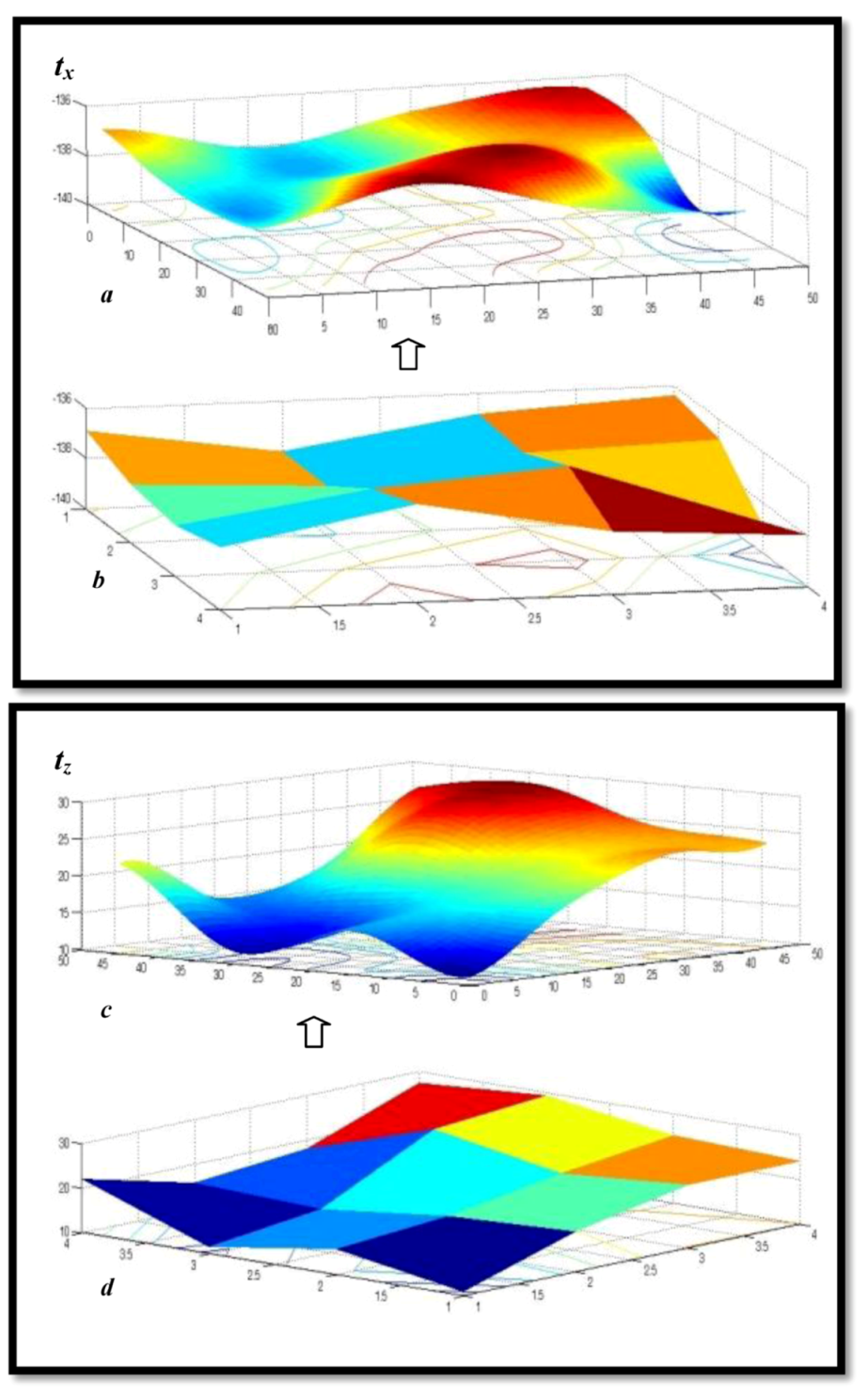
4.2.1. Translation Values

Due to the DTPM data structure—the DTM look-like model—an interpolation that will ensure continuous parameter representation has to be chosen. Interpolating DTM heights using bi-directional third degree parabolic equations is described in [18]. This algorithm is an area-based one that ensures smooth interpolation within a grid-cell, as well as excluding surface representation discontinuities on cell borders, while moving to neighboring cells. This algorithm is an improved version of the simplistic bi-linear area-based interpolation that might produce jagged and unsmooth surface representation.

This algorithm is designed for height interpolation; analogously, it can be altered to handle the three linear characterized translation values stored in the transformation matrix on three separate processes. Equation (8) depicts the algorithm’s equations utilized for this interpolation. Implementing this process enables us to accurately define for each grid-point of the source dataset the three translation transformation parameters and, hence, to receive a more detailed and smooth ‘translation surface’ that corresponds adequately to these translation values.

Returning to the “among” and “in-between” notations: first, this interpolation is implemented “among” the translation values in three separate processes for a specific position required for transformation; then, linear interpolation is carried out on each computed translation value in the “in-between” direction.

(8)

where F_k, while k ∈ [1–4] denotes the third-degree parabolic equations, Z_P denotes the value calculated by the interpolation at location, P, p_n, while n ∈ [x,y] denotes the normalized inner cell coordinates {0 ≤ p_n ≤ 1}, H(i,j) denotes the values stored in the grid-corner points and i, j while (i and j) ∈ [1–4] denote the index of four by four neighboring nodes.

4.2.2. Rotation Values

Euler angles representation are perhaps the most common parameterization of 3D orientation space. A naive approach to interpolating the rotation values might suggest independent and separate processes between each of the three Euler angles in order to produce the mediate positions needed. The outcome of this will produce a motion that is specified by a rotation that looks contracted, jerky at times, not continuous and ill-specified. This occurs mainly due to the fact that Euler angles ignore the interaction of the rolls about separate axes; hence, there is not a unique path between every two orientations across different coordinate systems; thus, there exists a dependency among the three-axis [19]. A resulting rotation depends on the order in which the three rolls are performed, which gives rise to further ambiguity that coincides with the fact that rotations in space do not generally commute.

The notation of quaternion is therefore given to define a 3-dimensional number system by a four-dimensional one [20] (it is worth noting that the translation of Euler angles representation to quaternion one involves several straightforward mathematical expressions). The four quaternion numbers describe a rotation followed by a scaling. Each quaternion object contains four scalar variables, which, hence, can be added and multiplied as a single unit in a similar way to the usual algebra of numbers. However, as with matrix algebra, quaternion multiplication is not commutative. Quaternions have four dimensions: one real and three imaginary. Each of the imaginary dimensions has a unit value of the square root of (−1), all mutually are perpendicular to each other, known as i, j and k. The notation of a quaternion is given in Equation (9), where W is the scalar part of the quaternion and (X,Y,Z) are the vector part with axes i, j and k. The main practical application of the notation of 4D quaternions was found to be in representing 3D rotations, while restricting it to those with unit magnitude.

(9)

The naive linear interpolation between two key quaternions will result in a straight line, which ignores the natural geometry of rotation space: the interpolated rotation would result in a motion that speeds-up in the middle. This is because linear interpolation is not in motion on the hyper-sphere surface, but, instead, cuts across it. The needed motion is a motion that does not speed-up, but keeps a constant velocity (i.e., zero acceleration) on it. This requirement translates itself geometrically into a great arc drawn between two given key unit-quaternions, i.e., spherical linear interpolation (SLERP), depicted in Figure 8, which ensures a unique and correct path under all circumstances [21], depicted in Equation (10):

(10)

where q₁ and q₂ are two key unit-quaternion orientations, θ is the angle between these vectors, q_i—which creates an angle, t, with q₁ (while t ∈ [0,1])—is derived from a spherical interpolation between vectors, q₁ and q₂.

SLERP is required for “in-between” interpolation between each given rotation value. A higher interpolation order for the DTPM matrix grid structure of orientations is required within a grid-cell, i.e., “among”. The idea is to calculate a sequence of SLERPs on the given unit-quaternions. This procedure enables the construction of a cubic as a series of three spherical linear interpolations of quadrangle of unit-quaternions on the surface of a 4D unit hyper-sphere. By doing so, the calculation of any mediate orientation by a series of SLERPs is achieved. Cayley [21] defined this procedure as spherical and quadrangle (SQUAD). Thus, having a grid of four corner-orientations {q₀,q₁,q₂,q₃}, three steps of the SLERP sequence can be suggested. This is equivalent to a Bezier curve with a spherical cubic interpolation, depicted in Equation (11). Still, quaternion multiplication is not a commutative one; so, the order in which this SQUAD sequence is implemented should be considered.

SQUAD(q₀,q₁,q₂,q₃,t) = SLERP(slerp(q₀,q₁,t),SLERP(q₂,q₃,t),2t(1 − t)

(11)

Figure 8. Conceptual representation of spherical linear interpolation (SLERP): instead of a naive linear interpolation (left) SLERP guarantees keeping constant velocity on the hyper-sphere surface (right).

Figure 8. Conceptual representation of spherical linear interpolation (SLERP): instead of a naive linear interpolation (left) SLERP guarantees keeping constant velocity on the hyper-sphere surface (right).

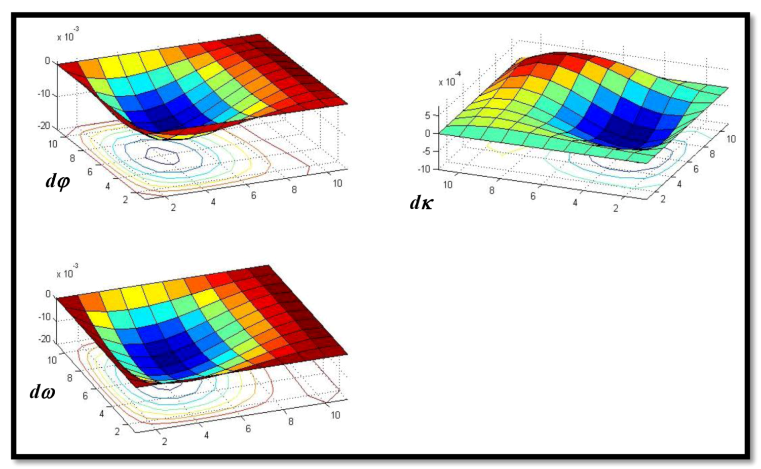
5. Statistical Analysis

Since the interpolation mechanisms discussed in Section 4.2.1 and Section 4.2.2 are not specifically designed for transformation parameters interpolation stored in the DTPM, this section aspires to verify that, indeed, they can be used for this purpose. Moreover, as discussed in Section 4.2.2, quaternion multiplication is not commutative, thus, there might exist some constraints as to the SQUAD sequence implemented; this is analyzed and described in Section 5.2.

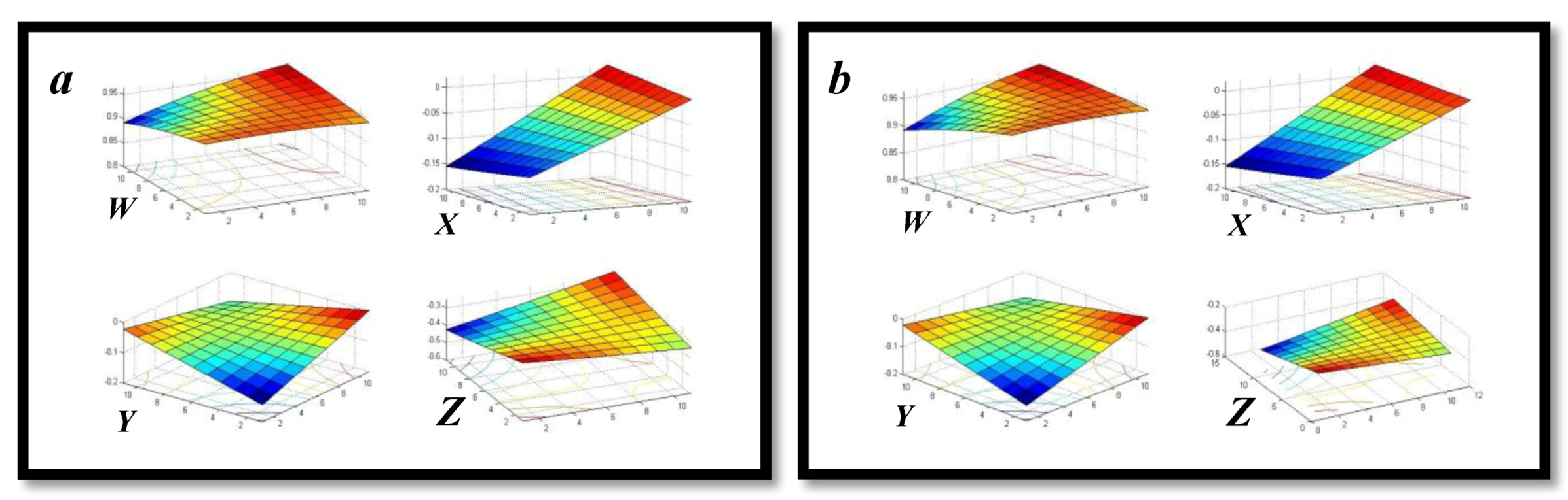
5.1. Translation Parameters

Two examples of the suggested bi-directional third degree parabolic interpolation are depicted in Figure 9. The source data is a DTPM transformation matrix with a resolution of 700 m, which is derived from using 1 km² frames (with approximately 30% overlap) ICP process. The desired resolution of 50 m is derived from the used DTMs. Calculating the translation values for a specific location (i.e., “among”), while shifting from the 700 m matrix grid resolution to the desired 50 m DTM resolution, preserves continuity, guaranteeing smooth interpolation within the entire coverage area. The output is a more detailed and continuous translation value calculation on the entire area required for the computation of the intermediate topography.

Figure 9. Bi-directional third degree parabolic interpolation for translation values t_x (left) and t_z (right). (b) and (d) are displayed in the original 700 m DTPM resolution, while (a) and (c) are displayed in the resulting 50 m resolution needed for morphing and blending.

Figure 9. Bi-directional third degree parabolic interpolation for translation values t_x (left) and t_z (right). (b) and (d) are displayed in the original 700 m DTPM resolution, while (a) and (c) are displayed in the resulting 50 m resolution needed for morphing and blending.

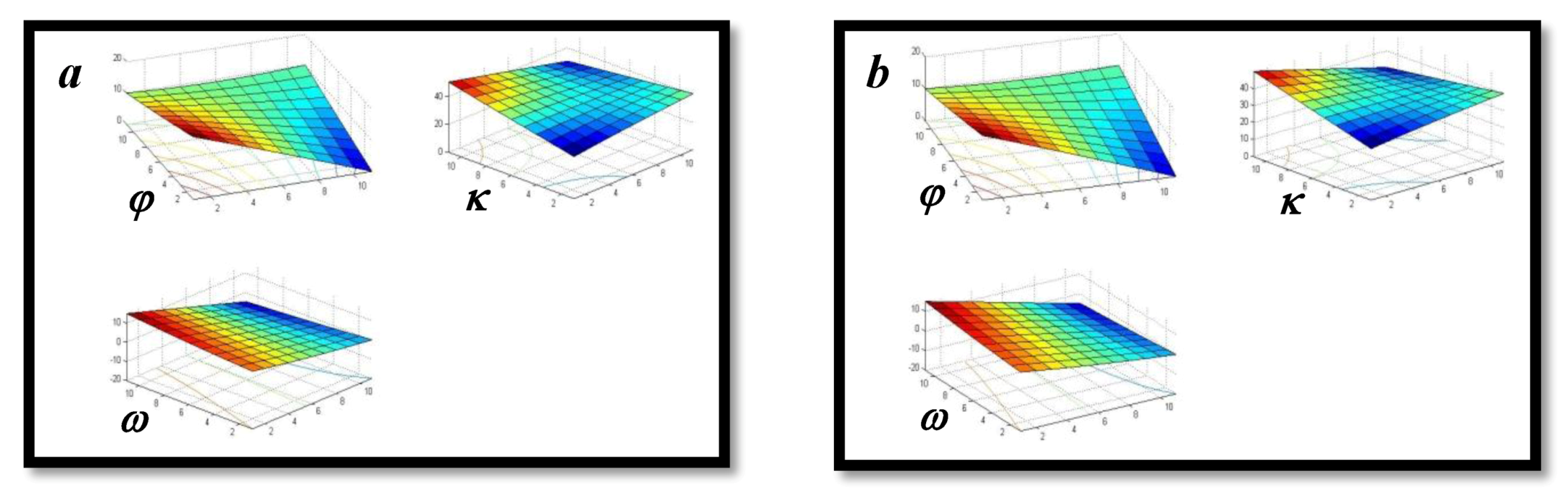
5.2. Rotation Parameters

Since quaternion multiplication is not commutative, the order of how the SLERP interpolations are carried out within each SQUAD implementation might have influence on the resulting rotation values and, thus, affecting the reliability of the animation produced with the creation of topographic artifacts. For example, while relying on the fact that the matrix grid size used in the interpolation is 700 m wide (as in Section 5.1), an erroneous resulting interpolation difference value of one decimal degree will result in a maximum position shift of six meters.

To quantify this inadequacy, a synthetic analysis evaluation is carried out, in which large registration values of rotation angles were taken into account. Large values were deliberately used to ascertain the reliability of this interpolation mechanism used. Figure 10 schematically depicts this, while the four corners represent a single DTPM cell with the rotation registration values used. An 11 by 11 grid was generated covering the cell (total of 121 positions), in which for each position, two SQUAD sequence calculations were implemented: interpolation sequence a—two SLERPs on the two horizontal couples (q₁-q₂ and q₄-q₃), followed by a SLERP on the resulting quaternions values; and, b—two SLERPs on the two vertical couples (q₁-q₄ and q₂-q₃) followed by a SLERP on the resulting quaternions values. This analysis is carried out to quantify and evaluate whether choosing a specific sequence (a or b) has any quantitative effect on the calculated interpolation values outcome, i.e., measuring the attributed commutative error. Thus, for all 121 positions, two sets of four unit-quaternion coefficients values are calculated (W,x,y,z); consequently, three Euler angle values, (φ,κ,ω) are generated, enabling the quantitative analysis of the differences these two sets of rotation values have.

Figure 11 depicts a mesh representation of all 121 four unit-Quaternion coefficients values calculated via the two SQUAD sequences—a and b. Visually comparing these two sets—left and right, respectively—no significant differences are evident. When comparing the values received, a maximum difference value of 0.01 in the W coefficient exists with significant lower difference values for all remaining coefficients. Moreover, it is apparent that the values are smooth and continuous within the entire cell area with no abrupt change in value.

Figure 12 depicts all 121 three Euler rotation angles values received via the two SQUAD sequences—a and b (after translating them from the quaternion 4D domain). Inspecting the values received, there are no significant differences for all three coefficients: a maximum of 0.004 decimal degrees. The values are smooth and continuous within the entire cell area, with no abrupt change in value.

Figure 10. DTPM single cell with two spherical and quadrangle (SQUAD) sequences given as parabola-motion form (arcs)—orientation nodes q_i {i ∈ [1–4]} values (φ,κ,ω) in degrees.

Figure 10. DTPM single cell with two spherical and quadrangle (SQUAD) sequences given as parabola-motion form (arcs)—orientation nodes q_i {i ∈ [1–4]} values (φ,κ,ω) in degrees.

Figure 11. Four unit-quaternion coefficient values calculated via two different SQUAD sequences—a (left) and b (right) (a and b are denoted as parabola motion in Figure 9).

Figure 11. Four unit-quaternion coefficient values calculated via two different SQUAD sequences—a (left) and b (right) (a and b are denoted as parabola motion in Figure 9).

Figure 12. Three Euler angles values calculated via two different SQUAD sequences—a (left) and b (right) (a and b are denoted as parabola motion in Figure 9).

Figure 12. Three Euler angles values calculated via two different SQUAD sequences—a (left) and b (right) (a and b are denoted as parabola motion in Figure 9).

Figure 13 depicts the value differences between the three Euler rotation angles received via the two SQUAD sequences. Though slight value changes do exist—average angular difference of approximately 4 × 10⁻³ decimal degrees—these values are not significant enough to have an effect on the procedures suggested here: with DTPM cell size used in the interpolation of 700 m wide, the resulting “among” interpolation difference value will have an effect of less than 2 cm on the shifting values (1:35,000 in scale). Carried out on large coverage DTMs with resolutions of dozens to hundreds of meters, the resulting outcome is still highly reliable.

It is visible in Figure 13 that on the border of the cell, the differences are zero, suggesting the process is correct (the SQUAD on the borders is actually translated into SLERP implementation). The Difference values increase toward the center of the cell, which is a result of the SQUAD and SLERP mathematical notions. Table 1 depicts the mean and standard deviation (SD) values computed for these angular differences.

It is worth emphasizing that the rotation values stored in the DTPM are normally smaller than the ones used in this analysis: normally, several decimal degrees with respect to the dozens used here. Thus, it can be concluded that using quaternion space and SLERP and SQUAD interpolation concepts is reliable and produces qualitative results; thus, it contributes to the mechanism and concepts implemented here.

Figure 13. Difference values between the three Euler angles calculated via two different SQUAD sequences—values in decimal degrees (z-axis).

Figure 13. Difference values between the three Euler angles calculated via two different SQUAD sequences—values in decimal degrees (z-axis).

Table 1. Mean and SD angular difference values for the two different SQUAD sequences.

Parameter	Difference values
	Mean	SD
dφ (deg)	−0.0033	0.0041
dκ (deg)	0.00005	0.0003
dω (deg)	−0.0042	0.0048

Table 1. Mean and SD angular difference values for the two different SQUAD sequences.

Parameter	Difference values
	Mean	SD
dφ (deg)	−0.0033	0.0041
dκ (deg)	0.00005	0.0003
dω (deg)	−0.0042	0.0048

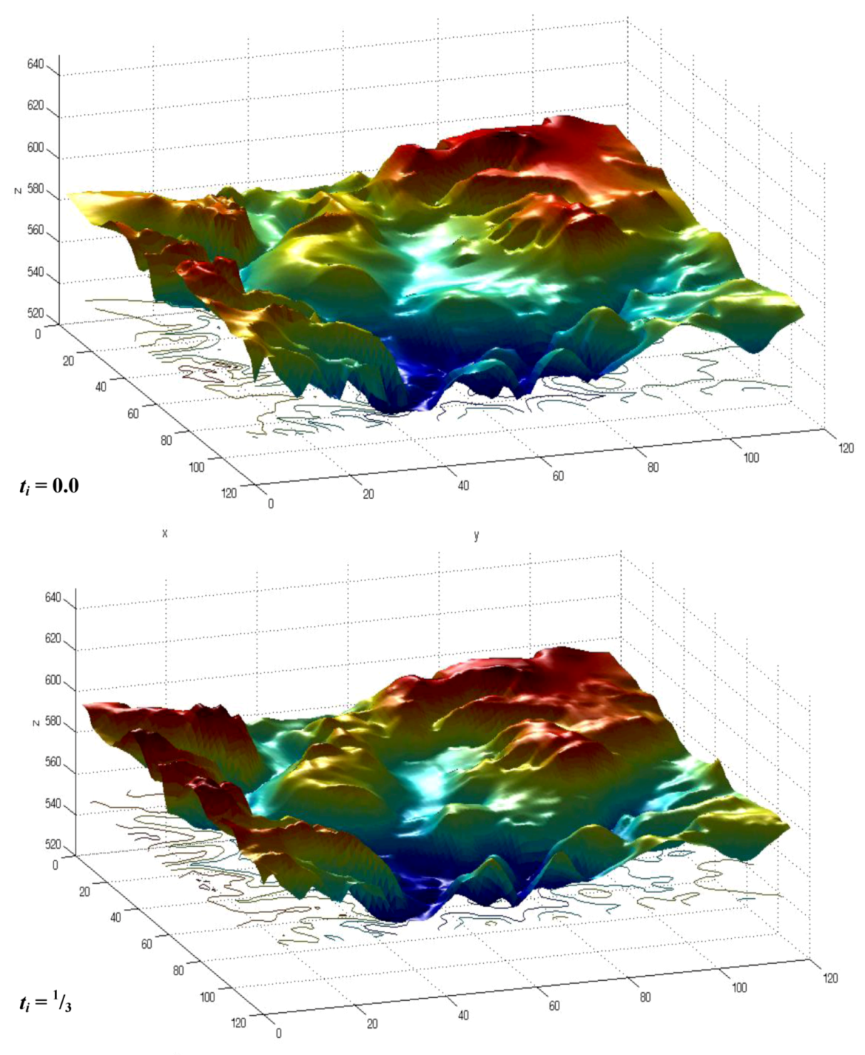
6. Results

The entire process was programmed with a Matlab R2013a working environment and implemented on a standard PC working station (Windows 7 with i5 processor and 4G RAM). The duration of processing time is dependent on the DTM coverage area analyzed. A single process, i.e., interest point identification, registration, matching and interpolation to a specified intermediate position, on two DTMs with coverage area of approximately 100 km² takes less than 60 s. Though not developed to have real-time capabilities, with the required programming language and processing unit (C++ and server workstation, for example), this scheme might present near real-time potential for the processing of a relatively small to medium area; based on previous experience and tests, the entire processing time can be reduced to a sub-second.

One can assume that two given topographic datasets represent two epochs: t₀ = 0 and t₁ = 1, respectively (source and target). Knowing the complete local interrelations (correspondence) between these “times”, which are stored in the DTPM, enables the calculation of any hypothetical temporal intermediate position (or scene) t_i (while t_i ∈ [0,1], where, theoretically, i ∈ [0,∞]) along the vertex path source-to-target. The produced intermediate topography is true to the geometries existing, as well as to morphologic alterations occurring (vertex correspondence). This enables complete and comprehensive 3D visualization and construction of multi-temporal topography simulation via the interpolation on all six transformation values corresponding to each point in the source dataset that is transformed to its predicted position in the target.

Figure 14. Intermediate scene t_i = ¹/₃ (bottom row) produced, while using data stored in source (t₀ = 0.0, top row) and target topographic datasets (t₁ = 1.0, Figure 14 bottom row) and DTPM (figures are with no scale, z-axis in meters).

Figure 14. Intermediate scene t_i = ¹/₃ (bottom row) produced, while using data stored in source (t₀ = 0.0, top row) and target topographic datasets (t₁ = 1.0, Figure 14 bottom row) and DTPM (figures are with no scale, z-axis in meters).

Figure 15. Intermediate scene t_i = ²/₃ (top row) produced while using data stored in source (t₀ = 0.0, Figure 13 top row) and target topographic datasets (t₁ = 1.0, bottom row) and DTPM (figures are with no scale, z-axis in meters).

Figure 15. Intermediate scene t_i = ²/₃ (top row) produced while using data stored in source (t₀ = 0.0, Figure 13 top row) and target topographic datasets (t₁ = 1.0, bottom row) and DTPM (figures are with no scale, z-axis in meters).

Figure 14, Figure 15 demonstrate the proposed intermediate scene visualization on two DTMs, both covering an area of 40 km². The source DTM was produced via photogrammetric means using low resolution satellite imagery, while the target DTM was produced via digitization of a 1:50,000 height contours map. Both DTMs present a resolution of 50 m and approximately the same level of accuracy. The top row in Figure 14 displays the source DTM (t₀ = 0.0), while the bottom row in Figure 15 displays the target DTM (t₁ = 1.0). The complete fully-automatic hierarchical modeling mechanism is implemented, resulting in the extraction of the complete different levels of geometric interrelations and correspondence of both DTMs stored in the DTPM (translation values extracted are: t_x = 124.6 m (~2.5 resolution cells), t_y = −50.1 m (~1 cells) and t_z = 30.0 m; all rotation values are several decimal degrees). The visualization of “times”, t_i = ¹/₃ and t_i = ²/₃, is presented—bottom row in Figure 14 and top row in Figure 15, respectively—while using all six transformation parameters and the designed interpolation concepts. While source and target topographies present different morphologies and representation, the result presents a natural transition in space between the two physical surfaces, overcoming non-realistic artifacts that might occur otherwise. The intermediate scene visualization resembles the morphological features existent, spatially transforming and deforming (morphing and blending) from one topography to the other.

Moreover, a series of intermediate scenes can be produced, while visualizing from t₀ = 0.0 to t₁ = 1.0 at ∆t interval scenes. The smaller ∆t is (∆t→0), the more continuous the transition presented by the intermediate scenes will be. Combining these scenes together will result in an animation sequence of all transition states, i.e., scenes, from one topography to the other. This can give knowledge about the hypothetical morphological changes, which occurred between the two given topographic dataset epochs. An example carried out on the above topographic datasets with an interval of ∆t = 0.01, e.g., 100 intermediate scenes, can be viewed at: http://youtu.be/ZdTU8saqaV4.

7. Conclusions and Discussion

Standard off-the-shelf GIS and animation applications designed to model topographic datasets are mostly based merely on the datasets’ mutual coordinate reference systems and on simplified geometric set of rules. This is usually in contrast to the physical reality and alterations these datasets model and represent. The commonly used “flip-page” concept does not try to attempt solving mutual existing relations, but rather only to produce an abstract and simplified simulation and representation. Shape blending and shape morphing algorithms will usually require a manual intervention, solving the complexity required.

The proposed hierarchical modeling mechanism, on the other hand, uses a different level of correlations and interrelations that are automatically a priori locally modeled. These reliable and robust set-of-correspondences are defined as a digital transformation parameters model used for accurate and reliable time-dependent visualization of multi-temporal intermediate scenes, i.e., simulation and animation. Several interpolation algorithms are introduced, which are designed for correct data-handling of the discrete transformation values stored in the DTPM, thus enabling continuous geo-oriented simulation analysis to be executed.

The hierarchical modeling mechanism enables us to quantify precisely the inaccuracies and discrepancies exist between the topographic datasets via the concept of using several consecutive levels of spatial modeling. This enables us to extract the existing mutual correlations and, hence, monitoring and modeling phenomenon that are characterized only locally for a more reliable and qualitative true-to-nature multi-temporal visualization. It is worth noting that this concept is not solely restricted to visualization implementations only, as other various accurate and reliable geo-oriented GIS analysis tasks can be implemented based on this novel mechanism.

References

- Mach, R.; Petschek, P. Visualization of Digital Terrain and Landscape Data: A Manual, 1st ed.; Springer: Heidelberg, Germany, 2007. [Google Scholar]
- Nebiker, S. Support for Visualisation and Animation in a Scalable 3D GIS Environment: Motivation, Concepts and Implementation. In Proceedings of ISPRS Workshop on Visualization and Animation of Reality-Based 3D Models, Vulpera, Switzerland, 24–28 February 2003.
- Stasko, J.T. The path-transition paradigm: A practical methodology for adding animation to program interfaces. J. Visual. Lang. Computing 1990, 1, 213–236. [Google Scholar] [CrossRef]
- Turk, G.; O’Brien, J.F. Shape Transformation Using Variational Implicit Functions. In Proceedings of the 26th Annual Conference on Computer Graphics and Interactive Techniques, Los Angeles, CA, USA, 8–13 August 1999; pp. 335–342.
- Thomas, F.; Johnston, O. Disney Animation: The Illusion of Life; Disney Editions: New York, NY, USA, 1981. [Google Scholar]
- Mohr, A.; Gleicher, M. Building efficient, accurate character skins from examples. ACM Trans. Graph. 2003, 22, 562–568. [Google Scholar]
- Watt, A.; Watt, M. Advanced Animation and Rendering Techniques; ACM: New York, NY, USA, 1992. [Google Scholar]
- Wang, R.; Pulli, K.; Popovi, J. Real-time enveloping with rotational regression. ACM Trans. Graph. 2007, 26, 73/1–73/9. [Google Scholar]
- Yu, Y.; Zhou, K.; Xu, D.; Shi, X.; Bao, H.; Guo, B.; Shum, H.Y. Mesh editing with poisson-based gradient field manipulation. ACM Trans. Graph. 2004, 23, 644–651. [Google Scholar] [CrossRef]
- Gomes, J.; Darsa, L.; Costa, B.; Velho, L. Warping & Morphing of Graphical Objects (The Morgan Kaufmann Series in Computer Graphics and Geometric Modeling); Morgan Kaufman: San-Francisco, CA, USA, 1998. [Google Scholar]
- Lazarus, F.; Verroust, A. Three-dimensional metamorphosis: a survey. Visual Comput. 1998, 14, 373–389. [Google Scholar] [CrossRef]
- Wolberg, G. Image morphing: A survey. Visual Comput. 1998, 14, 360–372. [Google Scholar] [CrossRef]
- Alexa, M.; Cohen-Or, D.; Levin, D. As-Rigid-As-Possible Shape Interpolation. In Proceedings of the 27th Annual International Conference on Computer Graphics and Interactive Techniques, New Orleans, LA, USA, 25–27 July 2000; pp. 157–164.
- Zhang, H.; Sheffer, A.; Cohen-Or, D.; Zhou, Q.; van Kaick, O.; Tagliasacchi, A. Deformation-Driven Shape Correspondence. In Proceedings of Symposium on Geometry Processing 2008, Copenhagen, Denmark, 2–4 July 2008; pp. 1431–1439.
- Zöckler, M.; Stalling, D.; Hege, H.C. Fast and intuitive generation of geometric shape transitions. Visual Comput. 2000, 16, 241–253. [Google Scholar]
- Dalyot, S.; Doytsher, Y. A Hierarchical Approach toward 3-D Geospatial Data Set Merging. In Representing, Modelling and Visualizing the Natural Environment: Innovations in GIS 13; Mount, N., Harvey, G., Aplin, P., Priestnall, G., Eds.; CRC Press/Taylor & Francis Group: Boca Raton, FL, USA, 2008; pp. 195–220. [Google Scholar]
- Besl, P.J.; McKay, N.D. A method for registration of 3-D shapes. IEEE Trans. Pattern Anal. Mach. Intell. 1992, 14, 239–256. [Google Scholar] [CrossRef]
- Doytsher, Y.; Hall, J.K. Interpolation of DTM using bi-directional third-degree parabolic equations, with FORTRAN subroutines. Comput. Geosci. 1997, 23, 1013–1020. [Google Scholar] [CrossRef]
- Foley, J.D.; van Dam, A.; Feiner, S.K.; Hughes, J.F. Computer Graphics Principles and Practice, 2nd ed.; Addison-Wesley: Reading, MA, USA, 1990. [Google Scholar]
- Cayley, A. An Elementary Treatise on Elliptic Functions; Dover Publications: New York, NY, USA, 1961. [Google Scholar]
- Shoemake, K. Animating Rotation with Quaternion Curves. In Proceedings of Proceedings of the 12th Annual Conference on Computer Graphics and Interactive Techniques, San Francisco, CA, USA, 22–26 July 1985; Volume 19, pp. 245–254.
© 2013 by the authors; licensee MDPI, Basel, Switzerland. This article is an open access article distributed under the terms and conditions of the Creative Commons Attribution license (http://creativecommons.org/licenses/by/3.0/).
Share and Cite
Dalyot, S.; Doytsher, Y. Multi-Temporal Time-Dependent Terrain Visualization through Localized Spatial Correspondence Parameterization. ISPRS Int. J. Geo-Inf. 2013, 2, 456-479. https://doi.org/10.3390/ijgi2020456
Dalyot S, Doytsher Y. Multi-Temporal Time-Dependent Terrain Visualization through Localized Spatial Correspondence Parameterization. ISPRS International Journal of Geo-Information. 2013; 2(2):456-479. https://doi.org/10.3390/ijgi2020456
Chicago/Turabian StyleDalyot, Sagi, and Yerach Doytsher. 2013. "Multi-Temporal Time-Dependent Terrain Visualization through Localized Spatial Correspondence Parameterization" ISPRS International Journal of Geo-Information 2, no. 2: 456-479. https://doi.org/10.3390/ijgi2020456