An Examination of Three Spatial Event Cluster Detection Methods

Abstract

In spatial disease surveillance, geographic areas with large numbers of disease cases are to be identified, so that targeted investigations can be pursued. Geographic areas with high disease rates are called disease clusters and statistical cluster detection tests are used to identify geographic areas with higher disease rates than expected by chance alone. In some situations, disease-related events rather than individuals are of interest for geographical surveillance, and methods to detect clusters of disease-related events are called event cluster detection methods. In this paper, we examine three distributional assumptions for the events in cluster detection: compound Poisson, approximate normal and multiple hypergeometric (exact). The methods differ on the choice of distributional assumption for the potentially multiple correlated events per individual. The methods are illustrated on emergency department (ED) presentations by children and youth (age < 18 years) because of substance use in the province of Alberta, Canada, during 1 April 2007, to 31 March 2008. Simulation studies are conducted to investigate Type I error and the power of the clustering methods.

1. Introduction

In disease surveillance, statistical methods can be used to identify geographical areas that have statistically higher numbers of cases of a disease than expected by chance. These geographical areas with aggregations of disease are called clusters. A geographical cluster is defined as a limited area within the general study area with a significant increase in the incidence of a disease (a hot spot cluster; see Lawson [1], p. 104). In some situations, the disease incidence or prevalence may not be the most or only relevant feature for analysis, and the analysis of events related to individuals with disease may be more appropriate. For example, when examining the delivery of health services through emergency departments (EDs), the number of presentations to EDs can be more relevant than the number of distinct individuals seen in the ED. If there are many individuals that have multiple presentations, analysis based solely on the number of individuals, and not the number of presentations, will only be able to identify clusters with excess numbers of individuals and not clusters with excess presentations. Ignoring presentations prevents the identification of clusters where more presentations, but not necessarily more individuals, are occurring than expected. Surveillance of presentations to EDs can identify geographic areas with high presentations, where access to other healthcare providers is limited, and statistical detection of these areas necessitates incorporating repeated presentations by individuals.

The geographical units of analysis are generally administrative regions for which case and population counts are available. Different methods of statistical tests have been proposed to locate and identify the clusters of disease cases in geographical areas. Besag and Newell [2] classified these statistical cluster detection tests as general (also called non-focused) and focused. General tests identify any cluster with an excess number of cases, whereas focused tests identify areas of excess cases near possible causative agents, such as environmental contaminants. There are a number of different tests that can detect clusters of cases when the geographic area has diverse population sizes (e.g., see [2–5]). When disease-related events are of interest, methods are required to accommodate the possibility of multiple, correlated events per individual. Tests for detecting clusters of events (hereafter, event cluster detection) are a relatively new research area, and a few approaches have been proposed. Rosychuk, Huston and Prasad [6] provided an event clustering test that is similar in spirit to the Besag and Newell [2] strategy, where areas are combined in order to contain at least a certain number of disease-related events. In their approach, the probability of observing the number of events is based on a compound Poisson distribution, and the relevant probabilities are obtained through a recursion relation. Building on this work, Torabi and Rosychuk [7] proposed the use of an approximate normal distribution to the compound Poisson distribution, and Rosychuk and Stuber [8] provided an exact test based on a multiple hypergeometric distribution.

We evaluate the performance of the three approaches for identifying geographic clusters of events. Section 2 describes the tests in detail, and Section 3 illustrates the methods on a dataset of ED presentations made by children and youth for substance use. Results of a simulation study are presented in Section 4, and a summary of the findings is provided in Section 5.

2. Materials and Methods

We first introduce some notation that is used for all methods. We consider a geographical study region divided into I distinct administrative areas, called cells. A crude spatial relationship amongst the cells is characterized by calculating pairwise distances between cell centroids. For cell i, i = 1, ⋯, I, the remaining cells are ordered in increasing distance from the cell’s centroid. Specifically, we let cell i_p be the p−th closest cell to cell i, p ∈ {0, 1, …, i − 1, i + 1, …, I}. For convenience, we define i₀ = i. The population of cell i is denoted by n_i, with total population $N={\displaystyle {\sum }_{i=1}^I{n}_i}$. For event clustering, we test the null hypothesis that every individual is equally likely to have events independently of the other individuals and the location of residence. Rejection of the null hypothesis suggests that the number of events is higher than expected by the event distribution. For cell i, let C_ix, x < ∞ be the random variable that represents the number of cases with exactly x events (observed value c_ix). The total number of cases with at least one event in cell i is C_i =∑_x C_ix, and the random variable V_i = ∑_x xC_ix denotes the number of events (observed value v_i). We assume that C_i and V_i are finite, and then, $C={\displaystyle {\sum }_{i=1}^I{C}_i}$ and $V={\displaystyle {\sum }_{i=1}^I{V}_i}$ denote the total number of cases and events for the entire region, respectively, with observed values of c and v.

Each cell is tested separately, similar in spirit to the method of Besag and Newell [2]. The test statistics are based on the number of cells required to be combined to include the nearest k^∗ events, where k^∗ is a natural number. For cell i, the test statistic is defined as:

$$L_i^{*}=\min \left\{q:k^{*}\le {\displaystyle \sum _{p=0}^q{V}_{i_p}}\right\}$$

(1)

The number of events in the combined cells can be considered as a sum of a random variable of the number of events. For cell i, suppose the number of cases and population in its l nearest neighbours, are $C_{il}={\displaystyle {\sum }_{p=0}^l{C}_{i_p}}$ and $n_{il}={\displaystyle {\sum }_{p=0}^l{n}_{i_p}}$, respectively. The total number of events for the n_il individuals can be written as:

$$V_{il}={\displaystyle \sum _{p=0}^l{V}_{i_p}}={\displaystyle \sum _{j=1}^{C_{il}}{Y}_j}$$

(2)

where Y_j is a random variable that denotes the number of events of the j−th (j = 1, …, C_il) individual.

2.1. Compound Poisson Distribution

The compound Poisson approach (CP) is the natural choice when thinking of the number of events in a cell and its neighbour as a random sum of random variables (Rosychuk et al. [6]). Since each case has at least one event and potentially many events, the significance level of each cell is determined by assuming that the number of events in the combined cells V_il has a compound Poisson distribution when C_il has a Poisson distribution. Therefore, V_il in Equation (2) has a compound Poisson distribution under the null hypothesis, and from Equation (1), the significance level becomes:

$$Pr\left(L_i^{*}\le l\right)=1-{\displaystyle \sum _{z=0}^{k^{*}-1}{P}_{il}(z)}$$

(3)

where P_il(z) = P r(V_il = z). Note that the probability P_il(z) in Equation (3) can be obtained through a recursion relation (see, for example, Ross [9], p. 156) where:

$$P_{il}(0)=e^{-{\mathrm{\lambda }}_{il}},$$

(4)

$$P_{il}(z)=\frac{{\mathrm{\lambda }}_{il}}{z}{\displaystyle \sum _{x=1}^{z}xQ(x)P_{il}(z-x),z\ge 1}$$

(5)

The probability Q(x) = Pr(Y_j = x) might be known by the investigator, and λ_il = n_ilC/N is the Poisson mean. We practically use ${\widehat{\mathrm{\lambda }}}_{il}=n_{il}c/N$ with the random variable replaced by that which is observed. Rosychuk et al. [6] used Q(x) = c_x/c, which c_x is the number of cases with exactly x events.

If the population distribution within the administrative area varies on key characteristics, such as gender and age, and these characteristics are available from both the population and case data, then these characteristics can be added to the test in order to adjust for the varying population distribution. Let C_•s be the random variable (observed value c_•s) that represents the number of cases in stratum s(s = 1, ⋯, S, S > 1) and n_•s be the corresponding total population in the entire region. For cell i, let n_isl and C_isl be the number of population and cases of stratum s and its l nearest neighbours, respectively. The random variable C_isl (observed value c_isl) follows a Poisson distribution with mean λ_isl = n_islC_•s/n_•s, and:

$$V_{il}={\displaystyle \sum _{s=1}^S{\displaystyle \sum _{j=1}^{C_{isl}}{Y}_{js}}}$$

(6)

is the total number of events for the C_il cases. V_il follows a compound Poisson distribution, with Y_js equal to the number of events of the j−th individual in stratum s, j = 1, ⋯, C_isl with probability Q_s(x) = Pr(Y_js = x) for all j and events x ≥ 1. Thus, the required probabilities can be determined from Equations (4) and (5) with the aid of Q(x) = Q₁(x)λ_i1l/λ_il +·⋯·+Q_S(x)λ_iSl/λ_il, and the corresponding significance test can be obtained by Equation (3).

2.2. Approximate Normal Distribution

When the population size is large, there may be relatively large numbers of events that can cause the calculation of the recursion relation Equations (4) and (5) to be slow. The computation time increases when we have strata with auxiliary information. Using an approximate normal (AN) (Torabi and Rosychuk [7]) approach provides an alternative to the CP approach. That is, the total number of events for the n_il individuals $V_{il}={\displaystyle {\sum }_{j=1}^{C_{il}}{Y}_j}$ in Equation (2) has a normal distribution with mean μ_il and variance ${\mathrm{\sigma }}_{il}^2$, and we can write the mean and variance of V_il as:

$${\mathrm{\mu }}_{il}={\mathrm{\lambda }}_{il}{\displaystyle \sum _{x=1}^{\infty }xPr(Y=x)=}{\mathrm{\lambda }}_{il}{\displaystyle \sum _{x=1}^{\infty }xQ(x)}$$

(7)

and:

$${\mathrm{\sigma }}_{il}^2={\mathrm{\lambda }}_{il}{\displaystyle \sum _{x=1}^{\infty }{x}^{2}Pr(Y=x)=}{\mathrm{\lambda }}_{il}{\displaystyle \sum _{x=1}^{\infty }{x}^{2}Q(x)}$$

(8)

where Q(x) = Pr(Y_j = x) is discussed in Section 2.1. Therefore, the significance level becomes:

$$Pr(L_i^{*}\le l)=1-\mathrm{\Phi }\left(\frac{k^{*}-0.5-{\mathrm{\mu }}_{il}}{{\mathrm{\sigma }}_{il}}\right)+\mathrm{\Phi }\left(\frac{-0.5-{\mathrm{\mu }}_{il}}{{\mathrm{\sigma }}_{il}}\right)$$

(9)

where Φ(·) is the cumulative standard normal distribution. The significance level in Equation (9) can be computed using the estimates ${\widehat{\mathrm{\mu }}}_{il}$ and ${\widehat{\mathrm{\sigma }}}_{il}^2$ of the parameters mean μ_il and variance ${\mathrm{\sigma }}_{il}^2$. As a result,

$${\widehat{\mathrm{\mu }}}_{il}={\widehat{\mathrm{\lambda }}}_{il}{\displaystyle \sum _{x=1}^{\infty }xQ(x)=\frac{n_{il}c}{N}\times \frac{1}{c}{\displaystyle \sum _i{\displaystyle \sum _{x}x{c}_{ix}=\frac{n_{il}v}{N}}}}$$

(10)

and:

$${\widehat{\mathrm{\sigma }}}_{il}^2={\widehat{\mathrm{\lambda }}}_{il}{\displaystyle \sum _{x=1}^{\infty }{x}^{2}Q(x)=\frac{n_{il}c}{N}\times \frac{1}{c}{\displaystyle \sum _i{\displaystyle \sum _x{x}^2{c}_{ix}=\frac{n_{il}{v}^{*}}{N}}}}$$

(11)

with $v_i^{*}={\displaystyle \sum _x{x}^2{c}_{ix}}$ and $v^{*}={\displaystyle \sum _i{v}_i^{*}}$.

When strata are included in the analysis, V_il in Equation (6) has a normal distribution with mean ${\mathrm{\mu }}_{il}={\displaystyle {\sum }_{s=1}^S{\mathrm{\mu }}_{isl}}$ and variance ${\mathrm{\sigma }}_{il}^2={{\displaystyle {\sum }_{s=1}^S\mathrm{\sigma }}}_{isl}^2$, where μ_isl and ${\mathrm{\sigma }}_{isl}^2$ can be obtained respectively from Equations (7) and (8) with λ_isl = n_islC_•s/n_•s defined above. Thus, a significance test similar to Equation (9) can be obtained. In particular, for both CP and AN methods, Q_s(x) can be estimated by c_•sx/c_•s, where c_•sx is the number of cases with exactly x events in stratum s.

2.3. Multiple Hypergeometric Distribution

For an exact approach, Rosychuk and Stuber [8] considered the event frequencies as classes, and subjects are sampled without replacement form the classes. This approach leads to a multiple hypergeometric distribution. The probability of observing x events among a sample of m individuals is:

$$M(x,m)={\displaystyle \sum _{\mathcal{A}}\frac{\left(\begin{array}{c}{C}_{•1}\\ r_1\end{array}\right)\left(\begin{array}{c}{C}_{•2}\\ r_2\end{array}\right)\cdots \left(\begin{array}{c}{C}_{•Y}\\ r_Y\end{array}\right)\left(\begin{array}{c}n-C\\ m-r_1-r_2\cdots r_Y\end{array}\right)}{\left(\begin{array}{c}n\\ m\end{array}\right)}}$$

(12)

where $C_{•y}={\displaystyle {\sum }_{i=1}^I{C}_{iy}}$ is the total number of cases in the entire study region with exactly y events, and {r_y} are non-negative integers from the set $\mathcal{A}$with:

$$\mathcal{A}=\left\{(r_1,\cdots ,r_y):x={\displaystyle \sum _{z=1}^{Y}z{r}_z}and{r}_y\le C_{•y,}y=1,\cdots ,Y\right\}$$

The significance level for the tested cell i becomes:

$$Pr(L_i^{*}\le l)=1-{\displaystyle \sum _{x=0}^{k^{*}-1}M(x,n_{il})}$$

(13)

Hereafter, we refer to this approach as the exact event (EE) test. In practical situations, the random variables are replaced by their corresponding observed values, and the expected number of events n_ilv/N is helpful. Further, suppose that V_is is the number of events in cell i for strata s, and the number of events in cell i is $V_i={\displaystyle {\sum }_{s=1}^S{V}_{is}=}{\displaystyle {\sum }_{s=1}^S{\displaystyle {\sum }_{z=1}^{Y}z{C}_{isz}}}$, with C_isx as the random variable denoting the number of cases in cell i that have exactly x events. When strata are taken into account, the test statistic in Equation (1) applies, and a significance test similar to Equation (13) will be obtained with the relevant probability expressed in Equation (12).

2.4. Selection of Cluster Size

The event cluster detection tests described all depend on the choice of cluster size, k^∗, which will not be known. The choice of k^∗ is crucial since a too large or too small choice may result in missing clusters. Le, Petkau and Rosychuk [10] recommend a testing algorithm that has multiple, cell-specific cluster sizes that depend on the population of the cell and its neighbors. We provide a description of the algorithm in the context of the different tests.

Let $k_{i0}^{*}$, $k_{i1}^{*}$ and $k_{i2}^{*}$ be the selected event cluster sizes for cell i, i = 1, ⋯, I. In a similar fashion to sequential analysis, cell i is tested at $k_{i0}^{*}$, $k_{i1}^{*}$, $k_{i2}^{*}$ in sequence only if an earlier cluster size fails to reach significance. Let $k_{iw}^{*}-1$ be the 100(1 − α) percentile of the events probability distribution f(·) with populations from the cell and up to its w nearest neighbours. The event cluster size $k_{iw}^{*}$ is the smallest, integer defined as:

$$k_{iw}^{*}=1+\max \left[q:{\displaystyle \sum _{z=0}^{q}f(\cdot )}\le 1-\alpha \right]$$

(14)

A cluster size equal to $k_{iw}^{*}$ is interpreted as the minimum number of events that would have to be observed to cause cell i and its nearest w neighbours to be significant at level α. The f(·) in Equation (14) would be replaced by the appropriate distribution of the specific method used. For the EE method, the event cluster size is defined as:

$$k_{iw}^{*}=1+\max \left[q:{\displaystyle \sum _{z=0}^{q}M(x,n_{iz})}\le 1-\alpha \right]$$

(15)

where M(x, n_iz) is defined in Equation (12).

3. Application to Substance Use Data

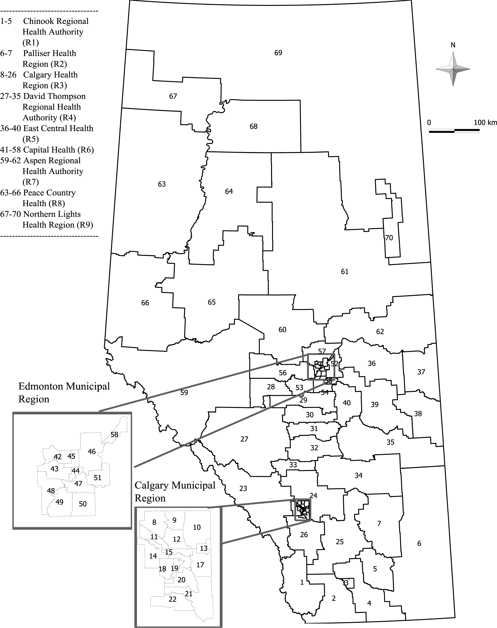
To demonstrate the behavior among the three methods, we focus on ED presentations by children and youth (years of age < 18) for substance use in the western Canadian province of Alberta during 1 April 2007, to 31 March 2008. Alberta has a population of over 3.5 million [11] and covers 661,848 km² [12]. The capital city, Edmonton, is located near the geographic center of the province, and Edmonton and Calgary are the two major urban areas, with populations over one million each. The southwestern boundary of the province has the Rocky Mountains, and the northern areas are forested and sparsely populated.

The data were extracted from population-based provincial administrative databases that include all ED presentations in Alberta. Each ED presentation during the study period is considered to be an event. A case is defined as an individual with at least one ED presentation for substance use during the study period. Since there are well-known differences between children and adolescents and males and females [13], we stratified the data by gender (male or female) and age group (0–14, 15–17 years of age). The province of Alberta (Figure 1) is divided into I = 70 sub-Regional Health Authorities (sRHAs) with diverse population sizes. The 25th percentile, median and 75th percentile of the sRHA population sizes are 5704, 10,832 and 18,027 residents, respectively, and ranged from 2225 to 31,828. The total children and youth numbered N = 862,771 in the population, and the total cases numbered c = 1232. The cases presented v = 1354 times to the ED with substance use. The majority of the individuals had three or fewer presentations: one (1128), two (83) or three (17). The range of presentations was from one to five. For each sRHA, the median number of cases was 14 (range zero to 52), and the median number of events was 15.5 (range zero to 59) [13].

We chose w to be at most two for our application and used hyperev [14] and R [15] statistical software packages to obtain the results. The statistically significant clusters (p-value < 0.05) are presented in

Table 1. Event cluster results with gender and age group as strata. Significant cells (i) in any approach along with the cluster size ( $k_{iw}^{*}$), test statistics (l), the number of observed events (v_il), the number of expected events (E_il) and corresponding p-value, with * denoting test significant at α = 0.05. CP, compound Poisson; AN, approximate normal; EE, exact event.

i	CP					AN					EE
	$k_{iw}^{*}$	l	vil	Eil	p-value	$k_{iw}^{*}$	l	vil	Eil	p-value	$k_{iw}^{*}$	l	vil	Eil	p-value
1	11	0	13	5.50	0.031*	11	0	13	5.50	0.037*	11	0	13	5.50	0.039*
2	19	0	24	11.73	0.030*	19	0	24	11.73	0.037*	19	0	24	11.73	0.045*
7	60	2	60	50.08	0.050*	64	3	65	58.70	0.285	64	3	65	58.70	0.275
25	42	1	44	32.75	0.042*	88	4	97	128.87	1.000	44	1	44	32.75	0.048*
27	15	0	22	9.02	0.047*	16	0	22	9.02	0.027*	16	0	22	9.02	0.035*
29	25	0	36	17.16	0.049*	26	0	36	17.16	0.034*	26	0	36	17.16	0.041*
30	33	1	39	24.70	0.047*	35	1	39	24.70	0.037*	35	1	39	24.70	0.042*
44	26	0	59	18.03	0.037*	27	0	59	18.03	0.035*	27	0	59	18.03	0.042*
45	78	2	107	67.64	0.050*	84	2	107	67.64	0.040*	85	2	107	67.64	0.040*
46	41	0	51	31.32	0.031*	43	0	51	31.32	0.035*	43	0	51	31.32	0.039*
47	55	1	84	42.07	0.041*	54	1	84	40.72	0.035*	55	1	84	42.07	0.044*
53	29	1	39	20.61	0.036*	30	1	39	20.61	0.038*	30	1	39	20.61	0.044*
56	44	0	44	34.22	0.033*	58	3	80	85.30	0.997	58	3	80	85.30	0.999
57	64	2	80	53.97	0.050*	69	2	80	53.97	0.037*	68	2	80	53.97	0.049*
58	60	2	64	49.55	0.035*	64	2	64	49.55	0.039*	63	2	64	49.55	0.049*
59	26	0	44	18.04	0.049*	28	0	44	18.40	0.027*	28	0	44	18.40	0.034*
60	62	1	64	51.16	0.028*	83	3	100	91.26	0.797	83	3	100	91.26	0.804
61	28	0	37	19.47	0.030*	29	0	37	19.47	0.038*	28	0	37	19.47	0.038*
62	37	0	59	27.67	0.032*	39	0	59	27.67	0.031*	38	0	59	27.67	0.050*
65	17	0	20	10.15	0.031*	17	0	20	10.15	0.037*	17	0	20	10.15	0.045*
66	44	0	50	34.72	0.047*	47	0	50	34.76	0.035*	47	0	50	34.72	0.039*
69	11	0	12	5.33	0.027*	11	0	12	5.33	0.032*	11	0	12	5.33	0.033*
70	32	0	32	23.14	0.032*	56	1	69	42.31	0.037*	56	1	69	42.61	0.040*

, along with the event cluster size k^∗, test statistic l, the number of observed events v_il, the number of expected events (E_il) and the p-value.

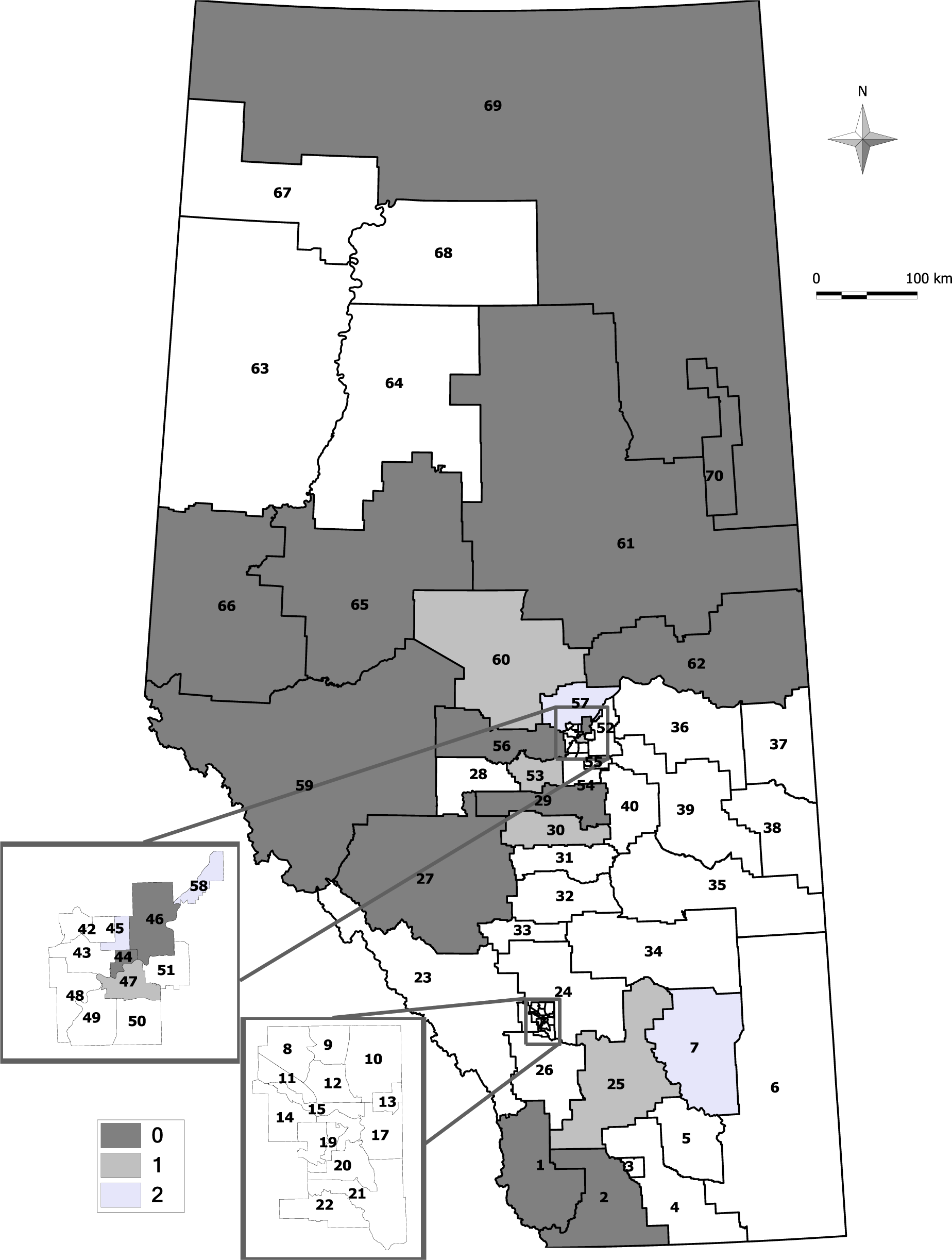
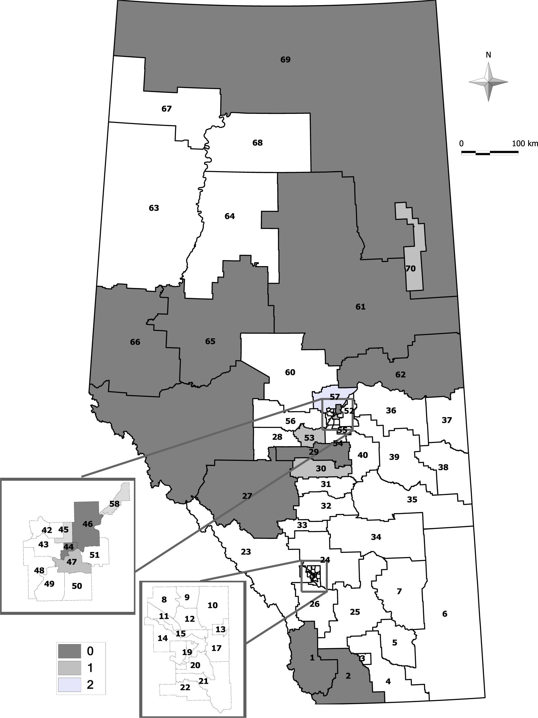
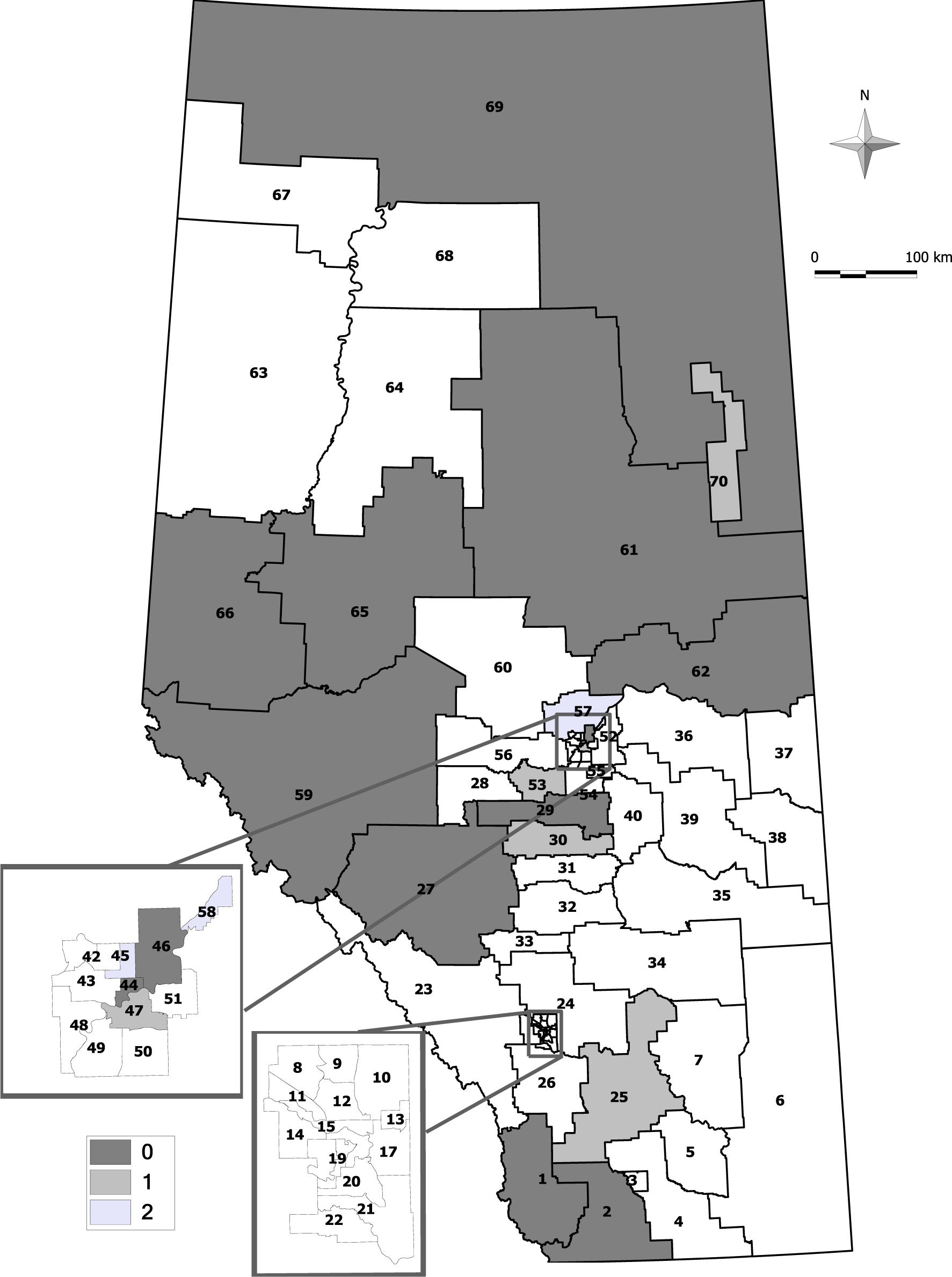
Almost all three methods identified geographical areas in the northeast and southwest areas of the province as statistically-significant clusters during the study period; few of the same sRHAs in the Edmonton Municipal region were identified as clusters of ED presentations, but none of the sRHAs were identified as a significant cluster in the Calgary Municipal region. A couple of geographical areas in the south were identified as single-cell potential clusters among all three methods, and a few other different sRHAs were identified as clusters from each approach (see Figures 2–4).

A few sRHAs had discrepant results among the three methods. These were likely because the CP and EE approaches have lower 95% tails than the AN approach. If the cluster sizes differ, then there may not be quite enough cases observed to meet statistical significance, and different numbers of cells may need to be combined. For example, sRHA 25 is identified as a significant cluster with its first nearest neighbour combined for the CP and EE approaches, but is not statistically significant for the AN approach. The sequence of cluster sizes ( $k_{i0}^{*}$, $k_{i1}^{*}$) tested for the CP, AN and EE approaches are (14, 42), (15, 45) and (14, 44), respectively. There are 13 events in sRHA 25 (< $k_{i0}^{*}$ for all approaches), and this observed number requires testing at $k_{i1}^{*}$. The first nearest neighbour of sRHA 25 is sRHA 26, and it contains 31 events. In combination, these two sRHAs have 44 events, and these exceed $k_{i1}^{*}$ for the CP and EE approaches. With the AN approach, $k_{i1}^{*}$= 45, and because 44 < 45, the next test occurs for $k_{i2}^{*}$ = 88. Continuing to combine neighbours until at least 88 events are observed, l = 4 neighbours need to be combined (sRHAs 26 (31 events), 21 (19 events), 17 (14 events), and 22 (20 events)), and this combination of sRHAs has 97 observed events (>88). With a larger number of neighbours (and a larger combined population size), the combined sRHAs do not have enough events to be identified as a statistically-significant cluster, and the p-value is less than 0.05.

It is important to note that merely having an observed number of events above the expected number of events does not guarantee that statistical significance is achieved. With the cluster size algorithm, statistical significance is achieved if the observed number of events is at least as large as the $k_{iw}^{*}$ and the l is ≤ w. For example in the AN and EE approaches, sRHA 60 needed to have at least 83 events when combined with its two nearest neighbours (w = 2) to be statistically significant. To achieve at least 83 events, its l = 3 nearest neighbours had to be combined with it. Although the observed number of events was 100 and the expected number of events was smaller at 91.26, this increase was not large enough for the combined populations to be identified as a statistically-significant cluster.

4. Simulation Studies

We examine the Type I error and the power of the tests of the CP, AN and EE approaches through simulation studies. The studies use Alberta’s cells and their geographic relationships. The cell populations are set to be the Alberta population for the fiscal year 2007/2008 or the same population (1000, 5000, or 8000) in each cell.

4.1. Type I Error Comparison

Five settings for the probability of multiple events per case were considered (

Table 2. Event probabilities for the simulation scenarios.

Scenario	Non-Zero Event Probabilities Q(x)
	Q(1)	Q(2)	Q(3)	Q(4)	Q(5)
S1	0.600	0.400	0.000	0.000	0.000
S2	0.600	0.250	0.150	0.000	0.000
S3	0.800	0.100	0.100	0.000	0.000
S4	0.800	0.150	0.040	0.010	0.000
S5	0.919	0.066	0.014	0.001	0.001

) with varying means and skewness chosen for convenience. Setting S5 is based on our substance use application. The events rate was set to be two events per 1000 population. That is, the total number of events in each simulated data set would be 140, 700, 1120 and 1354 for the setting with 1000, 5000 and 8000 per cell and the Alberta population, respectively. With the multiple event probabilities for scenarios S1–S5 from Table 2 and crude event rates, the simulated data sets are created by randomly assigning the c_•1, c_•2, ⋯, cases based on each cell’s proportion of the total population. For each simulation setting, we generated 1,000 datasets and applied the CP, AN and EE approaches to each dataset. We obtained the cluster sizes $k_{i0}^{*}$ for each approach and tested each cell only once to allow for clear comparisons. We provide the effective significance level α^∗ for each scenario (

Table 3. Simulation results for each cell size and scenario.

ni	Scenario	CP		AN		EE
		α*	SD	α*	SD	α*	SD
1000	S1	0.044	0.585	0.044	0.588	0.044	0.585
	S2	0.029	0.506	0.029	0.501	0.029	0.506
	S3	0.048	0.721	0.048	0.721	0.048	0.721
	S4	0.042	0.584	0.042	0.588	0.042	0.584
	S5	0.027	0.481	0.027	0.484	0.027	0.481
5000	S1	0.039	0.670	0.039	0.666	0.039	0.670
	S2	0.036	0.590	0.036	0.595	0.036	0.590
	S3	0.042	0.645	0.042	0.645	0.042	0.645
	S4	0.037	0.529	0.037	0.530	0.037	0.529
	S5	0.042	0.593	0.042	0.593	0.042	0.593
8000	S1	0.037	0.613	0.037	0.618	0.037	0.613
	S2	0.037	0.561	0.037	0.562	0.037	0.561
	S3	0.040	0.611	0.040	0.613	0.040	0.611
	S4	0.039	0.604	0.039	0.603	0.039	0.604
	S5	0.034	0.581	0.034	0.583	0.034	0.581
Alberta	S1	0.041	0.761	0.041	0.772	0.043	0.779
	S2	0.040	0.713	0.042	0.761	0.041	0.705
	S3	0.041	0.862	0.042	0.881	0.043	0.863
	S4	0.041	0.858	0.045	0.801	0.043	0.861
	S5	0.040	0.841	0.041	0.733	0.041	0.834

The effective significance level α^∗ is provided for each approach, and standard deviations (SDs) for the scenarios are given as percentages (%)

) based on the cluster size and provide the number of simulations that had at least one cluster detected with corresponding standard deviations (SDs).

For the scenarios with constant cell populations, the α^∗’s and the SDs are the same among the three methods. This result is to be expected, since the cluster sizes would be likely identical across the approaches, and the numbers of events per cell would be quite stable over the simulations. Across scenarios, the effective significance levels are close to 0.05. The effective significance levels are closer to 0.05 for the non-constant cell situation, where the Alberta population was used. For this data situation, the EE approach seems to perform slightly better than the CP and AN approaches for most of the scenarios considered. All results show that the detection rate of false clusters is close to what is expected by the significance level.

In practice, users of these methods will likely have datasets that have non-constant population sizes, although the sizes may not be as divergent as the Alberta population. The results suggest that the EE approach may be a better option to consider, although its computational requirements may be of concern if the population sizes are large and the number of events are high. The CP and AN approaches may have computational advantages that may surpass the Type I error advantage of the EE approach.

4.2. Power Comparison

In order to perform power comparisons among the three event cluster detection methods, we picked two of the sRHAs to be true clusters: sRHA 25 (in a rural area) and sRHA 44 (in an urban area). Using the simulated datasets from Section 4.1, we inflated the number of events in sRHAs 25 and 44 to create true clusters. The events were multiplied by two and 1.5 in sRHAs 25 and 44, respectively, and the ceiling was used if the multiplication resulted in a fractional number of events. This simulation approach allowed for a different distribution of events in the true clusters than the rest of the cells. A rate of 1.5-times higher than the overall rate is a commonly-used benchmark for urban areas. We calculated the power of the test for each true cluster separately as the number of simulations out of 1000 that correctly rejected the null hypothesis at the significance level α = 0.05.

Table 4. Estimated power of the CP, AN and EE methods for two different true clusters, for 1000 simulated datasets and for significance levels of 0.05.

ni	Scenario	sRHA25			sRHA44
		CP	AN	EE	CP	AN	EE
1000	S1	0.267	0.099	0.299	0.191	0.048	0.197
	S2	0.236	0.114	0.238	0.221	0.054	0.221
	S3	0.303	0.109	0.323	0.200	0.029	0.204
	S4	0.338	0.093	0.355	0.198	0.047	0.211
	S5	0.352	0.087	0.352	0.216	0.026	0.217
5000	S1	0.575	0.181	0.596	0.322	0.038	0.328
	S2	0.592	0.213	0.598	0.354	0.041	0.358
	S3	0.664	0.184	0.667	0.392	0.033	0.395
	S4	0.672	0.195	0.670	0.362	0.034	0.364
	S5	0.664	0.223	0.664	0.458	0.036	0.463
8000	S1	0.706	0.201	0.708	0.411	0.033	0.422
	S2	0.682	0.239	0.686	0.432	0.043	0.440
	S3	0.774	0.242	0.776	0.481	0.043	0.486
	S4	0.791	0.235	0.791	0.487	0.036	0.488
	S5	0.797	0.264	0.798	0.587	0.039	0.590
Alberta	S1	0.997	0.976	0.998	0.621	0.081	0.622
	S2	0.993	0.965	0.993	0.569	0.081	0.582
	S3	0.999	0.976	0.999	0.634	0.080	0.647
	S4	1.000	0.986	1.000	0.650	0.071	0.650
	S5	1.000	0.993	1.000	0.742	0.070	0.743

shows the results of the power analysis. For the constant cell population sizes, both the CP and EE approaches have higher power, while the power of the AN test is low. All tests perform better for the true cluster that has a higher rate. In particular, the AN method almost always identifies sRHA 25 for the Alberta population scenario and almost always fails to identify sRHA 44. The EE approach generally has higher power than the CP approach for all scenarios considered, but the extra computation may not be warranted when it only performs slightly better.

5. Discussion

The statistical cluster detection literature focuses on the detection of clusters of disease, and relatively few methods have been introduced to examine clusters of disease-related events, where the diseased cases may have multiple disease-related events. We have provided a comparison of three different event cluster detection methods. Each method follows the same overall testing scheme with different distributional assumptions: compound Poisson (CP), approximate normal (AN) and multiple hypergeometric (exact, EE). We used a testing algorithm adapted for each method. Our examination included an analysis on ED presentations for substance use in Alberta and a simulation study.

The CP method identified 23 potential clusters of ED presentations for substance use in Alberta children and youth during the fiscal year 2007/2008. The potential clusters were identified as clusters on their own or when combined with a small number of nearest neighbours. The other two methods identified slightly fewer potential clusters, and this result may be related to the probability in the tail of the relevant distributions. Based on this application, the CP method provides a greater number of potential clusters, although it is yet to be determined if these potential clusters are real or spurious (e.g., due to other potential factors that vary with sRHA, but are not adjusted for in the analysis). In real clusters, the areas identified in the less urbanized areas may indicate greater substance use or less availability of other health services. In the less urbanized areas, individuals may not be geographically close to health services or programs and may seek the ED for care. Particularly in the northwestern area of the province, there is a large geographic area and a relatively sparse population. Further investigation would be needed to determine potential causes of seemingly high numbers of ED presentations for substance use.

We conducted simulation studies to examine the likelihood of falsely detecting clusters. The simulation studies had different event probability distributions and different cell sizes that were either all the same or followed the population of Alberta. All three approaches had effective significance levels that were close to the specified level of 0.05. The methods seemed to be closer to 0.05 for the non-constant cell population setting, and in that setting, the EE approach had effective significance levels that were the closest to 0.05, compared to the other approaches for most scenarios.

We also used these simulation studies to perform a power investigation using two single-cell true clusters. In all situations, the CP and EE approaches were better than the AN approach. The AN approach was highly sensitive to the cell population sizes and performed well when population sizes were larger, and the true cluster had twice the rate of events. The AN approach would be best suited for finding clusters with high rates compared to the background. The CP and EE approaches also performed better for higher population sizes and higher rates. The EE approach was slightly better than the CP approach, but it is more computationally intensive and the benefit relatively small. Based on these results, the CP approach would be recommended for use, and like all clustering methods, clusters are more easily detected for higher rates and larger population sizes.

All methods used analogous cluster size testing algorithms. A benefit of the approach is that cluster sizes can be specific to each tested cell, which is important for geographic areas with diverse population sizes. A drawback of the approach is that each cell may be potentially tested at several sizes, thus increasing the multiple testing problem. It is noted though that the Monte Carlo simulations for the overall p-value use the same testing algorithm, and thus, the overall p-value is adjusted for multiple testing. Another benefit of the testing algorithm is that it allows the minimum cluster size to achieve statistical significance. For discrete distributions, this minimum may provide a number that is lower than the desired 0.05 significance level. With some differences in the distributions chosen, there is some variability in how close to 0.05 the p-values can be.

These methods use pairwise distances and a nearest neighbor ordering. Most of the calculations only involved the first few neighbors. This aspect provides advantages in the sense that the distances do not have to be precisely known, and the simulation studies would be applicable to other geographies, where the nearest neighbor ordering was the same. These aspects make our simulation results more generalizable to other geographic areas.

The limitations of our study include the necessity to pick a cluster size (or maximum number of cluster sizes to test) and the specification of scenarios for our simulation study. The testing algorithm allows the cluster sizes to be less sensitive to user choice, but still require the user to decide the maximum number of cells to combine as part of the selection of tested cluster sizes. This choice makes the results from the different methods a little less easy to compare, because the tested cluster sizes may be different among the three methods. It is also difficult to provide scenarios for the simulation study that correspond to every real data situation. The few scenarios presented provide the flavour of the behaviour of the methods under different conditions, and the performance may be not be illustrative for a particular data situation. In addition, we did not examine the power of the methods.

Our study does provide guidance to potential users of these three methods of the cluster detection of events. In the absence of strong distributional assumptions, the EE method may be the best for users to consider. Sensitivity analyses could also be done with the other distributions and would likely show similar results. In terms of health surveillance and policy, at least one of these methods could be included as part of a routine surveillance program of health-related events, such as ED presentations. If a geographic area has higher events than expected, it could be targeted for further investigation and/or intervention.

References

- Lawson, A.B. Statistical Methods in Spatial Epidemiology; John Wiley & Sons, Ltd.: Chichester, UK, 2001. [Google Scholar]
- Besag, J.; Newell, J. The detecting of clusters in rare diseases. J. R. Stat. Soc. Ser. A. 1991, 154, 143–155. [Google Scholar]
- Kulldorff, M.; Nagarwalla, N. Spatial disease cluster: Detection and inference. Statist. Med. 1995, 14, 269–286. [Google Scholar]
- Tango, T. A class of tests for detecting “general” and “focused” clustering of rare diseases. Stat. Med. 1995, 14, 2323–2334. [Google Scholar]
- Tango, T. A test for spatial disease clustering adjusted for multiple testing. Stat. Med. 2000, 19, 191–204. [Google Scholar]
- Rosychuk, R.J.; Huston, C.; Prasad, N.G.N. Spatial event cluster detection using a compound poisson distribution. Biometrics 2006, 62, 465–470. [Google Scholar]
- Torabi, M.; Rosychuk, R.J. Spatial event cluster detection using an approximate normal distribution. Int. J. Health Geogr. 2008. [Google Scholar] [CrossRef]
- Rosychuk, R.J.; Stuber, J.L. An exact test for the detection of geographic aggregations of events. Int. J. Health Geogr. 2010. [Google Scholar] [CrossRef]
- Ross, S.M. Introduction to Probability Models, 8th ed.; Academic Press: San Diego, CA, USA, 2003. [Google Scholar]
- Le, N.D.; Petkau, A.J.; Rosychuk, R.J. Surveillance of clusters near point sources. Stat. Med. 1996, 15, 727–740. [Google Scholar]
- Population and Dwelling Counts, for Canada, Provinces and Territories, 2011 and 2006 Censuses, Statistics Canada, Available online: http://www12.statcan.gc.ca/census-recensement/2011/dp-pd/hlt-fst/pd-pl/Table-Tableau.cfm?LANG=Eng&T=101&S=50&O=A accessed on 7 January 2015.
- Statistics Canada, Available online: http://www.statcan.gc.ca/tables-tableaux/sum-som/l01/cst01/phys01-eng.htm accessed on 7 January 2015.
- Newton, A.S.; Rosychuk, R.J.; Ali, S.; Cawthorpe, D.; Curran, J.; Dong, K.; Slomp, M.; Urichuk, L. The Emergency Department Compass: Children’s Mental Health, Available online: http://www.EDCompass.net accessed on 15 May 2013.
- Rosychuk, R.J. Hyperev: Statistical Disease Cluster Detection Program; Rosychuk: Edmonton, AB, Canada, 2007. [Google Scholar]
- R Core Team. R: A Language and Environment for Statistical Computing; R Foundation for Statistical Computing: Vienna, Australia, 2013. [Google Scholar]