1. Introduction
In recent years, urban road networks in many countries are becoming more congested [
1]. To alleviate traffic congestions, increasing attention has been given to developing intelligent transportation systems (ITS), with the aim to best use existing transportation networks through various advanced information technologies. The accurate and robust estimation of travel time information is critical to many ITS applications. The provision of updated travel time information enables travelers to make informed path choice decisions to avoid congested sites [
2,
3,
4]. Moreover, the updated travel time information allows for network operators to evaluate network performance, and to identify bottlenecks for proactively deploying effective controls so as to improve overall traffic conditions [
5,
6].
During the last few decades, various technologies have been developed to collect real-time travel time information [
7,
8]. Existing data collection techniques could be roughly classified into two categories: fixed traffic detection systems; and, floating car systems [
9,
10]. The fixed traffic detection systems employ conventional stationary detectors, such as loop detectors, installed at specific locations of road segments. These stationary detectors can continuously record every travel speed and traffic volume for all vehicles passing through the road segment with detectors. Because of their high installation and maintenance cost, stationary detectors are generally installed at only freeways or a few major roads. Thus, fixed traffic detector systems tend to have a small spatial coverage. Floating car systems are an emerging data collection technique, due to the recent advances in positioning and wireless communication techniques. The floating car system typically makes use of a large fleet of probe vehicles (e.g., thousands of taxis in a city), equipped with global positioning system (GPS) devices. The locations and speeds of moving probe vehicles are collected at a certain time interval to estimate travel time. The floating car systems are able to collect real-time travel time information for any part of the network where probe vehicles move. Due to the low operational cost and large spatial coverage, floating car data (FCD) recently has become a major data source for travel time estimation studies, as well as many ITS applications.
Travel time estimation methods have been intensively studied in the existing literature [
10]. Many effective methods have been proposed to estimate the mean travel times in freeways based on stationary detectors, including statistical methods and analytical methods [
11,
12,
13,
14,
15,
16,
17]. These travel time estimation methods for freeways, however, cannot be easily applied to urban road networks, mainly due to the following two reasons. Firstly, as mentioned above, stationary detectors are generally deployed at a few major roads, and are thus insufficient for estimating travel times in large-scale urban road networks. Secondly, travel times in congested urban road networks are highly stochastic, largely caused by the interruptions of signal controls at intersections. Many empirical studies have found that the stochastic nature of travel times in urban road networks have had a significant impact on travelers’ route choice behavior [
4]. The reliability of travel times has been recognized by network operators as one of the most important performance indicators. Nevertheless, the existing methods for estimating mean travel times in freeways ignore travel time variances, and thus are inadequate for estimating actual traffic conditions in urban road networks. Therefore, it is necessary to develop new methods for estimating both the mean and the variation of travel times (i.e., travel time distributions) in urban road networks using FCD.
In recent years, much attention has been given to developing travel time estimation methods based on the FCD [
1,
11,
15,
17,
18,
19,
20,
21]. Herring [
17] used FCD to estimate and predict traffic states, rather than link travel times. Sanaullah [
19] used FCD to study the influence of vehicle penetration rates, data sampling frequencies, vehicle coverage on the links, and time window lengths on the accuracy of link travel time. Zheng [
20] proposed a three-layer ANN model to estimate urban link travel times for individual probe vehicle data. Tang [
21] presented a method to estimate travel time based on low-frequency FCD. These travel time estimation methods based on FCD could provide effective mean travel times for a large-scale road networks, but travel time variances are still ignored.
To the best of our knowledge, only a few methods based on FCD have been developed to estimate travel time distributions in urban road networks. Jenelius [
1] presented a statistical model to estimate travel time in urban road networks based on low-frequency FCD. Both the mean travel time and 95% confidence intervals were given. Jenelius [
22] analyzed the estimation of path travel time distributions based on probe vehicle data sampled by time and space, and highlighted the difference between them. Rahmani [
15] developed a non-parametric method for route travel time distribution estimation using low-frequency FCD. The 25th, 50th, and 75th percentile values of the estimated travel time distributions were used to compare with that of the observed travel time distributions.
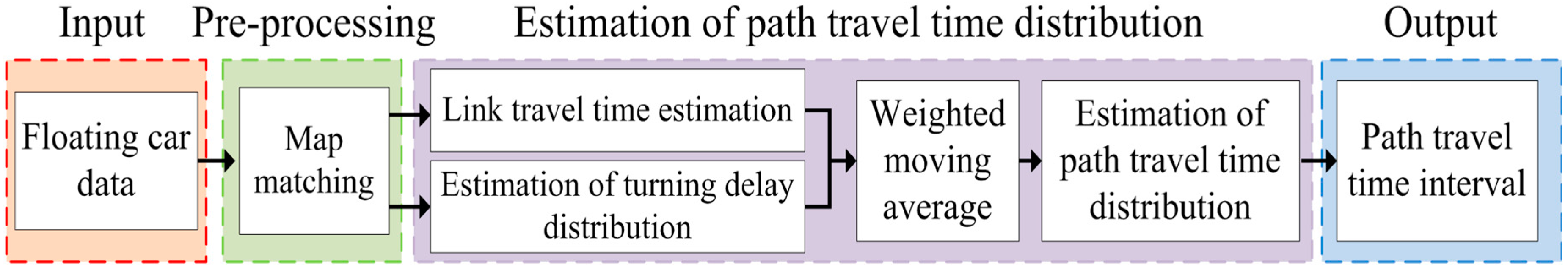
Along the line of previous work, this study proposes a robust method to estimate travel time distributions in urban road networks by using low-frequency FCD. Different from previous work, the path travel time distribution in this study is formulated as the sum of deterministic link travel times, and stochastic turning delays at intersections. Using this formulation, distinct travel time delays for different turning movements at the same intersection can be well captured. For example, left turns in China or USA (or right turns in the UK) are generally much more difficult than forward movements. The main contributions of this paper are summarized as follows.
Firstly, an effective method is proposed to estimate path travel time distributions based on low-frequency FCD. In this study, the path travel time distribution in this study is formulated as the sum of the deterministic link travel times and stochastic turning delays at intersections. A robust speed estimation algorithm based on the degree of central tendency is proposed to estimate deterministic link travel times. A distribution estimation algorithm is proposed to estimate the stochastic turning delays. Based on the arrival time of the intersection, α-discrete approximation method [
23] is utilized to generate the path travel time distribution.
Secondly, a weighted moving average algorithm is proposed to smooth deterministic link travel time and stochastic turning delays. Considering the low level of market penetration and the low sampling rate of probe vehicles, the sample size of FCD may not be sufficient in some time intervals. Thus, this method can provide a robust estimation and obtain reliable results.
Thirdly, to illustrate the applicability of the proposed method, a comprehensive case study is carried out using FCD from the Wuhan network. Two new indexes are employed to evaluate the accuracy of the estimated path travel time distributions. The experimental results show that the proposed method can obtain a reliable and accurate estimation of path travel time distribution in congested urban road networks.
The remainder of this paper is organized as follows. Problem statement of travel time distribution estimation is introduced in
Section 2. The proposed method to estimate travel time distribution is presented in
Section 3. A case study using real-world FCD collected at Wuhan, China is reported in
Section 4. Conclusions and recommendations for further research are given in
Section 5.
2. Problem Statement
A road network can be represented as a directed graph
, consisting of a set of
nodes
, a set of directed links
, and a set of allowed movements
. Each node
is a geographical location representing a network intersection, which can be either signalized or non-signalized [
24]. A link
is defined to be the road section from its tail node
to head node
. Its length is denoted by
, and its travel time, denoted by
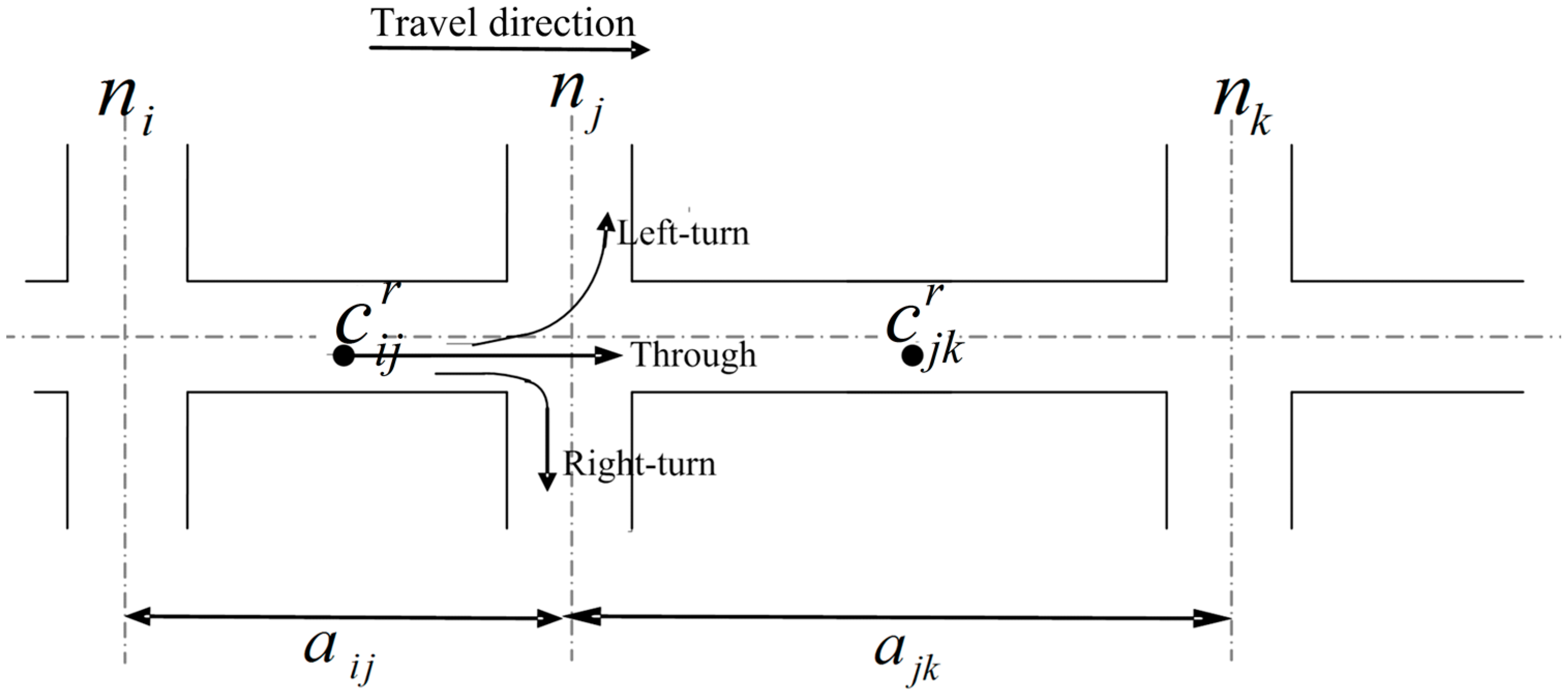
, is represented to be deterministic but varying with time of day. Each element
represents an allowed movement from tail link
to head link
, passing through node
. A movement
means that this movement is restricted in the road network (e.g., no U-turn). A movement
is assumed to have no physical distance, but it associates with a stochastic turning delay, denoted by
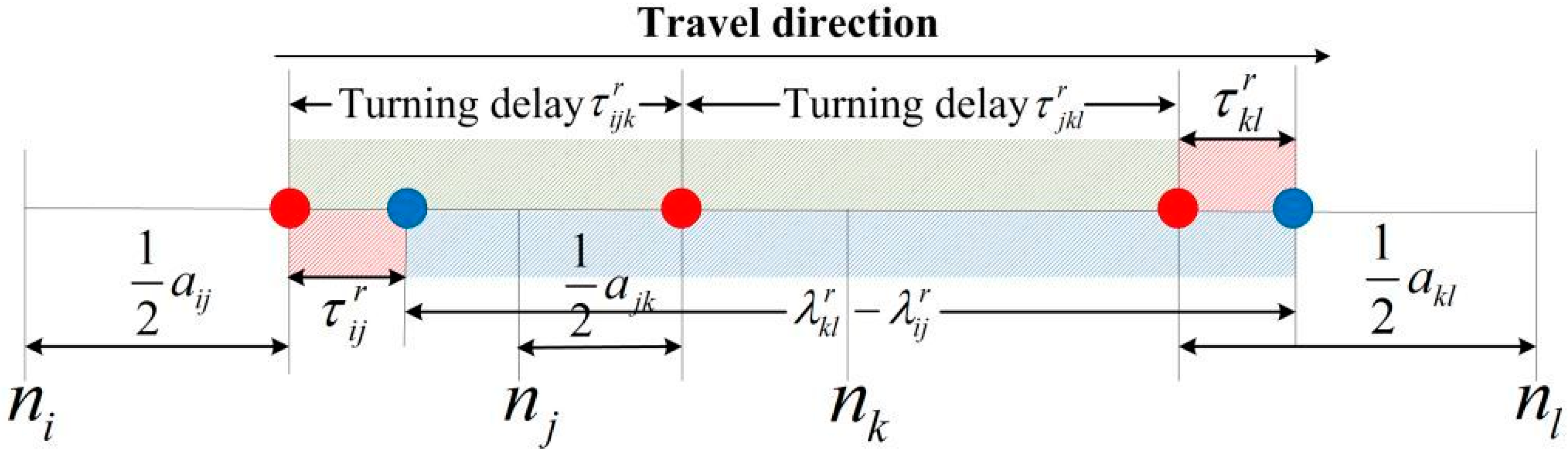
, varying with different probe vehicles and time of day. In this study, different movements (e.g., left-turn, through, and right-turn movements in
Figure 1) at the same node can have distinct turning delays.
Let
be a selected path from origin
to destination
. The path travel time, denoted by
, is the sum of the related link travel times and turning delays along the path as
where
and
are the arrival times at link
and node
respectively. As both arrival time and turning delays are stochastic time-dependent variables, the path travel time
is also a random variable conditionally depending on arrival times, link travel times and turning delays along the path.
In this study, trajectories of probe vehicles (i.e., FCD) are adopted to estimate the path travel time distribution,
, as well as associated link travel times and turning delay distributions along the path. As shown in
Figure 1, the trajectory of
probe vehicle consists of a set of GPS sampling points,
. Each GPS sampling point
compromises of a set of attributes, including time stamp
, instantaneous speed
, and geographic location in terms of latitude and longitude. This geographical location can be equivalently represented by a network location using the linear reference system in terms of a link
and a relative location
[
7]. For example,
indicates sampling point
is located at the middle of the link
. As illustrated in
Figure 1, there are two GPS sampling points,
and
, at adjacent links
and
. The time difference
between these two sampling points is the vehicle’s experienced travel time, which can be decomposed into two components: (1) deterministic travel times at these two network links,
, (2) and a stochastic turning delay
, experienced for movement
. Given a trajectory set of
probe vehicles during the same time interval, the observation set of link travel times and turning delay distributions can be generated. In next section, a robust method is proposed to estimate the path travel time distributions based on the observation set generated from FCD.
4. Case Study
The performance of the proposed model is investigated using numerical experiments. This section describes the experimental setup and discusses the experimental results.
4.1. Test Site and Data Collection
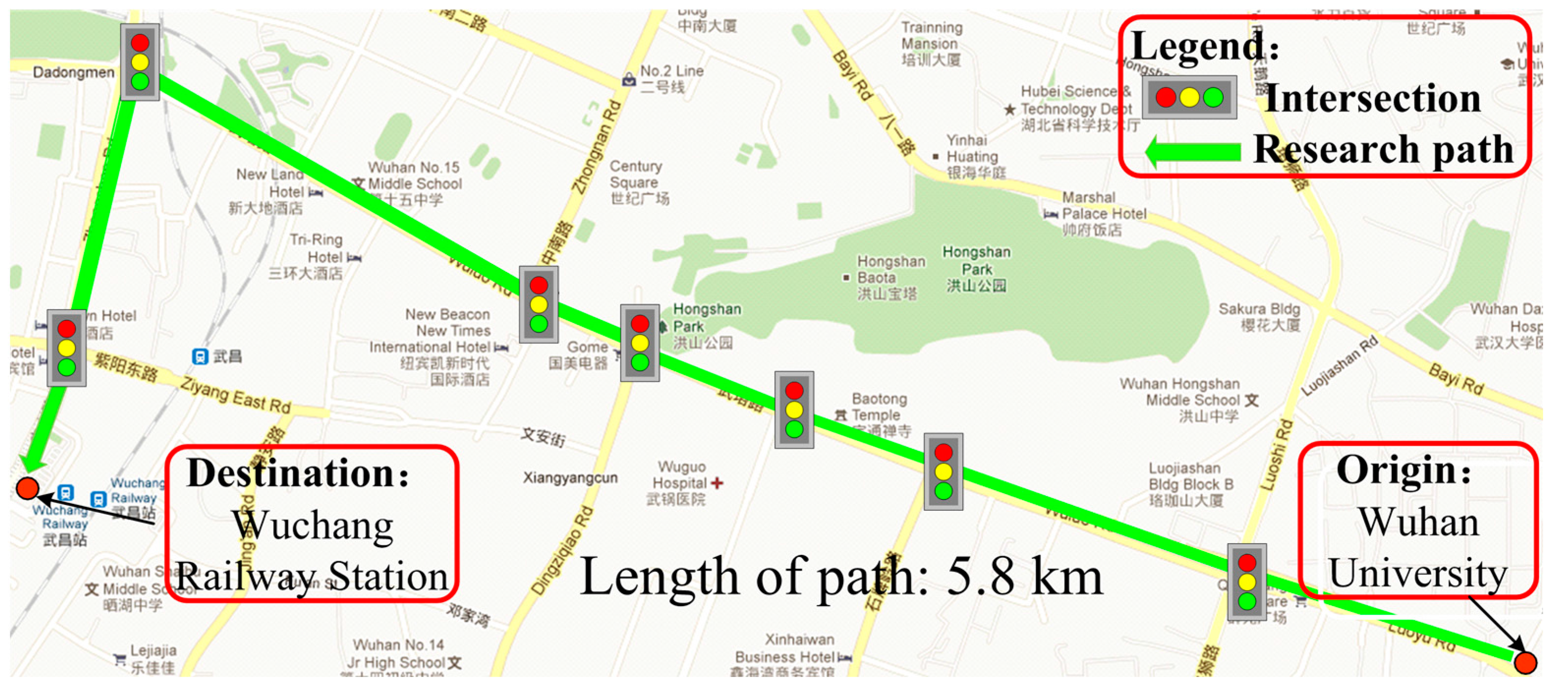
A real-world case study is reported in this section to demonstrate the applicability of the proposed distribution estimation method of turning delay and path travel time. The probe vehicle system in Wuhan, China is adopted for this case study. This probe vehicle system utilizes 11,245 taxis as probe vehicles, and the sampling time interval is about 40 s. 80% of the collected data are used to construct a model, and the rest of the data are test data. To validate performance of the proposed method, a major road (or path) from ‘Wuhan University’ to ‘Wuchang Railway Station’ (as shown in
Figure 6) was selected as the study path. This selected path consists of eight links and seven intersections, and its travel distance is 5.8 km. Travel times are estimated at 15-min interval from the morning peak to evening peak (07:00–22:00) of a typical weekday on 17 September 2009 (Thursday).
In this paper, the MM and the path inference algorithm [
28] are used. Chen et al., take into account the projection distance, network topology, and the shortest path comprehensively to determine the best candidate link. The proposed method is competitive with the existing FCD–MM algorithms with respect to both MM accuracy and computational performance.
Many studies assume that travel times follow for normal distribution [
23,
29]. Moreover, lognormal distribution is also a reasonable alternative. In congested urban road networks, travel times however are highly stochastic due to the fluctuations in traffic demand and supply, traffic control, and drivers’ varying behaviors, etc. Thus, the type of travel time distribution may be quite different at different locations in different periods. Based on these current studies, the path travel time and turning delay distribution are usually fitted with several classical distributions, namely normal distribution, lognormal distribution, and gamma distribution [
30,
31]. According to the Chi-square test, the best-fit results of turning delay distributions are shown in
Table 1. On the whole, the lognormal distribution is superior to the other two distributions at a 5% significance level. More than 50% of the distributions follow lognormal distribution, and the same results can be found in off-peak periods. In the morning and evening peak, the percentage of lognormal distribution decreases slightly, but is still dominant. The results show that normal distribution cannot describe a certain skew and long tail distribution [
16]. In conclusion, the assumption that all turning delay distributions obey the same distribution is unreasonable.
4.2. Evaluation Metrics
To quantify the accuracy assessment, two widely accepted metrics, namely, mean absolute percentage error (MAPE) and root mean square error (RMSE), were adopted to evaluate the accuracy of the estimated mean of path travel time distribution,
where
and
are the estimated and observed mean values of path travel times at time interval
, and
is the number of time intervals during the period of interest. Smaller
and
indicate a higher accuracy of the estimated mean path travel time.
The
MAPE and
RMSE concepts were extended to evaluate the accuracy of the estimated STD of the path travel time as followings,
where
and
are the estimated and observed STDs of path travel times at time interval
.
For many transportation applications, it is meaningful to construct a travel time interval at a given confidence level from the estimated or predicted travel time distribution [
32,
33]. The accuracy of travel time interval represents the integrated accuracy of both the estimated mean and STD. Two metrics were adopted to evaluate these accuracies: probability outside of the predicted (estimated) time interval (
POPI), and the probability outside of the observed time interval (
POOI) [
34]. The
POPI measures the percentage of observed data, or observed travel time interval outside of the estimated travel time interval, while the
POOI measures the percentage of estimated distribution outside of the observed travel time interval.
Let represent the estimated travel time interval. The lower and upper bounds are and , respectively, at confidence level , where is the inverse cumulative distribution function (CDF) of the estimated path travel time distribution. Similarly, the observed travel time interval is expressed as . and , respectively, which denote the lower and upper bounds of the observed travel time interval, at a confidence level of , where is the inverse of the CDF of the observed path travel time distribution. Let be the intersection between the estimated and observed travel time intervals. and are the lower and upper bounds of the intersection, respectively. For a certain time interval, and if .
In mathematical terms,
POPI is defined as follows,
where
denotes the CDF of the estimated travel time distribution. The
POPI value ranges from 0 to 1. The smaller
POPI indicates capture of larger proportion of observed data, i.e., higher accuracy of the estimated travel time interval. As noted by Shi [
34], this
POPI metric is very useful, but tends to exhibit bias for situations of wide travel time intervals due to large STD errors.
As an alternative, the
POOI measures the percentage of estimated distribution outside of the observed travel time interval.
denotes the CDF of the estimated travel time distribution. Accordingly,
POOI can be defined as
The POOI value also ranges from 0 to 1. The larger POOI value indicates the lower accuracy of the estimated travel time interval, because the larger proportion of estimated travel time interval is outside of the observed travel time interval. Therefore, these POPI and POOI matrices are complementary to evaluate the accuracy of the estimated path travel time interval.
4.3. Experimental Results and Analysis
This section reports the experimental results of the case study. In the proposed method, the sensitive parameter
in Equations (12) and (15) was set as 0.2, which is initially recommended by Dion and Rakha [
26], Tam and Lam [
27].
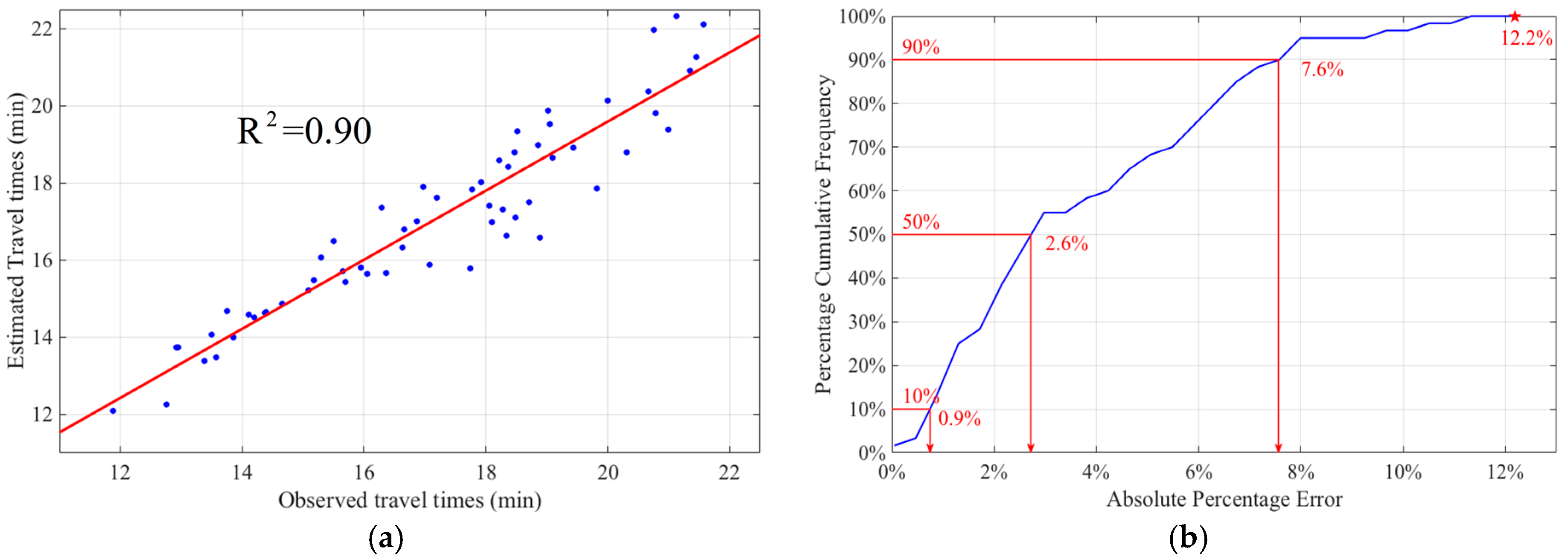
Figure 7a shows the path travel times estimated by the proposed method against the observed path travel times. The coefficient of determination (R
2) is 0.90, which reflects the accuracy of the estimated path travel times. It implies that 90% of the estimated path travel times are well fitted with the observed travel times on the study path during the period of interest. Moreover, the cumulative frequency distribution of the absolute percentage errors of the path travel times is depicted in
Figure 7b. It can be seen that half of the estimated travel times on the selected path are within 3% errors, whereas at least 90% of the estimated path travel times are within 8% errors. The estimation errors of the travel times on the selected path are all less than 13% in the study periods (as the red star shows). The proposed path travel time estimation method provided a reliable and accurate estimation of mean travel time,
, throughout the period of interest, with
. In summary, the performance of the proposed algorithm for urban travel time estimation is shown to be satisfactory.
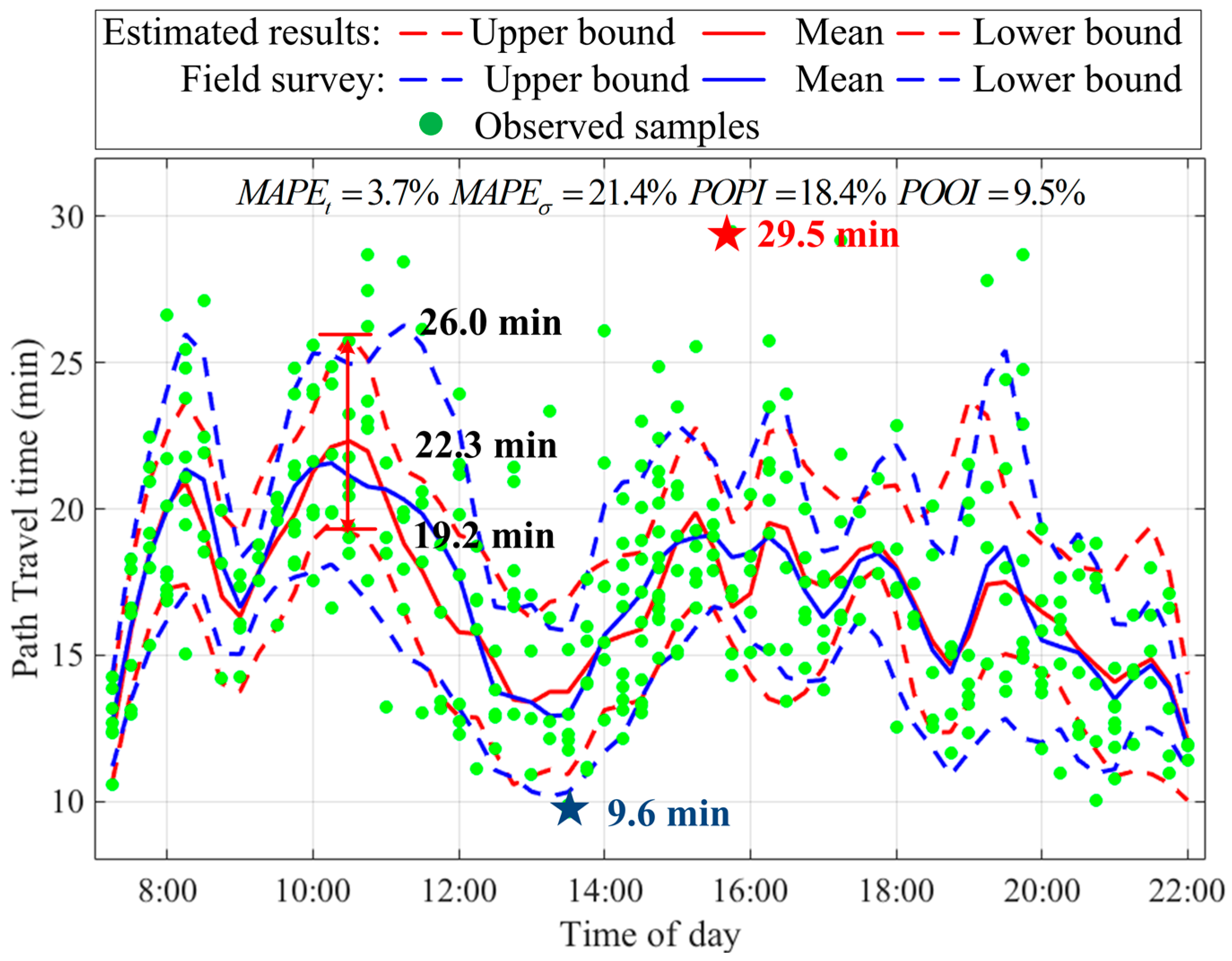
The upper and lower bounds of the estimated and observed path travel time intervals are given in
Figure 8. In this paper, the confidence level is equal to 80% (i.e.,
) due to two main reasons. On one hand, the travel time interval is determined by the level of confidence. Very narrow travel time intervals with a low confidence level are not reliable, while very wide travel time intervals with a high confidence level are not practically very useful. On the other hand, 10th and 90th percentile values of travel time distribution are usually used as the lower and upper bounds of travel time interval in the existing studies [
35,
36,
37,
38]. In
Figure 8, the constructed travel time intervals for both of the estimated and observed travel time distributions are shown in red and blue dotted lines, respectively.
POPI and
POOI metrics are also calculated for an 80% confidence level. Observed data from the field survey, shown in green dots, were only used for accuracy validation. As shown in the figure, the estimated travel time intervals can cover most observed data well during the period of interest. The proposed path travel time estimation method provided a reliable and accurate estimation of mean travel time,
, throughout the period of interest, with
. However, the relatively large
indicates that the proposed method has a bigger bias in estimation of path travel time distribution STD,
, for the period of interest. This highlights the challenge of accurately estimating
in congested road networks. One major reason may be the difficulty of estimating
of the population using biased and sparse samples. The
RMSEs of the mean and STD are 0.85 and 0.95 min, respectively. This indicates that the mean and STD of the estimated and observed path travel time distributions fluctuate within 1 min.
In terms of the accuracy of the estimated travel time interval, POPI is 18.4%, somewhat better than the target (20%), which indicates that a high proportion (81.6%) of observation data was well covered by the estimated path travel time interval. It can also be seen from the figure that the estimated interval was not too wide, given the relatively large STD error. POOI is equal to 9.5%, which is much smaller than the target (20%). Overall, the STD was underestimated, because the observation samples were relatively sparse. Thus, the POPI and POOI metrics demonstrate that the proposed method could obtain accurate and robust estimations of the path travel time interval (i.e., path travel time distribution).
It can be observed from
Figure 8 that the mean path travel time is stable, varying only from 12.1 min to 22.3 min. A lucky traveler may only require 9.6 min (as the blue star shows), while an unlucky one may even spend 29.5 min for the same trip (as the red star shows). For example, travelers want to take the train at 10:30 and set aside 10 min to check in, which means that travelers should arrive at Wuchang Railway Station at 10:20. The estimated mean travel time is 22.3 min, and the STD is 2.8 min. Based on the distribution of path travel times, travelers would choose appropriate departure times based on their attitudes of on-time arrival. Risk-seeking travelers (on-time arrival probability
is lower than 50%) tended to assign a small travel time budget for their trips. When
, risk-seeking travelers were assigned only 19.2 min travel time budget, which was 13.9% less than the expected travel time. However, the observed travel time was 21.6 min, and this was 2.4 min larger than the assigned travel time, which meant that risk-seeking travelers were almost late for their train. When
, the risk-averse travelers started their trips at 9:54, and this travel time budget was about 4.4 min larger than the expected travel time, that is, more time should be set aside to ensure a higher probability of on-time arrival. Therefore, it is necessary to provide not only the mean path travel time but also the variation of travel time distribution to travelers, so that they can make an informed trip planning decision.
The study demonstrated through Chi-square tests that the assumption of lognormal distribution is consistent with field travel time observations, and that lognormal distribution is representative of urban travel times under both light and heavy traffic conditions.
5. Conclusions and Further Studies
Provision of link or path travel time distribution information is a crucial requirement for travelers to make reliable route choice decisions incorporating travel time uncertainty. With advances in information and communication technologies (ICT), floating car systems, such as probe vehicles, are widely used in congested urban road networks. These floating car data collected from floating car systems are beneficial for robust and accurate estimation of travel time distribution information.
This paper addressed the problem of estimating travel time distribution in congested urban road networks using low-frequency FCD. In this study, the link travel time was modeled as a deterministic variable without consideration of interruptions caused by signal timing at intersections. Such interruptions due to signal timing were considered in delays of different turning movements at intersections. In this way, turning delays of different turning movements (through, right turn, and left turn) were modeled as random variables and fixed into lognormal distribution, which was consistent with field travel time observations validated through Chi-square tests. In addition, a weighted moving average method was proposed to provide a reliable and robust estimation of link travel time and turning delay distribution, considering that a sample size of FCD may be not sufficient. A speed estimation algorithm using the degree of central tendency instead of coverage proportion is presented to estimate the link travel time. A -discrete approximation method is utilized to generate the path travel time distribution.
A case study using real-world FCD collected in Wuhan, China was carried out to demonstrate the applicability of the proposed travel time estimation method. The results of the case study indicated that the lognormal distribution could provide a satisfied fitting for path travel time distribution, and turning delay distribution in congested urban road networks. Also, the results validated that the proposed method could obtain robust and accurate estimation of path travel time distribution over the whole period of interest. Compared with the observed travel time distribution, the estimation errors were quite low with respect to and metrics.
In the future study, the existing research can be extended in the following ways. First, travel times in this study were assumed to follow lognormal distributions for all time periods. However, several previous studies have found that the travel times in congested road networks could be better represented by normal, gamma, or Burr distributions [
39]. These distributions may be suitable for different time periods. Second, fusing traffic data from multiple sources to estimate or predict travel time distribution is also a significant challenge [
34]. Last but not the least, travel time distributions were estimated in this study for the current time interval. Extension of the proposed method to the problem of short-term travel time distribution prediction is another interesting topic for further study.


