1. Introduction
Remote sensing technology is developing rapidly as an efficient method for acquiring data from a distance, usually from outer space by a satellite. It is now becoming a popular tool for natural resource surveys, which determine the distribution and quantity of various natural resources over a specific area, such as soil, grassland, forest, and farmland. Remote sensing is making this process quicker, more efficient, and more economical, by providing a wide range of imageries varying in resolution and spectral band, and with the help of land cover classification and spatial analysis techniques [
1,
2,
3].
The first task to be completed before conducting a remote sensing-based survey is choosing an appropriate remote sensing data source to determine the imagery resolution and spectral bands, which have a significant effect on the accuracy of land cover classifications [
4]. The influence of spectral bands on the extraction and visualization of ground features, which are physical objects on the ground such as forest and water, is well known. For example, red and near-infrared bands are used to calculate the Normalized Difference Vegetation Index (NDVI) for vegetation detection or different band combinations of Landsat Thematic Mapper (TM) imagery are employed to highlight different ground features. However, the selection of the resolution, or the size of pixels that constituting an imagery, remains an unsolved problem. There is no “one size fits all” solution [
5], because the resolution should be determined with respect to the size of ground features, and there is one optimal resolution for each ground feature. If a unique resolution is adopted for all the ground features, details of objects smaller than the resolution would be lost.
Currently, several methods are used for determining the size of ground features such as semivariograms, local variance (LV), wavelet method, and spatial autocorrelation [
6,
7,
8]. Among them, semivariograms are widely adopted because of their mathematical simplicity and ease of interpretation. The
range of a semivariogram is related to the size of the ground feature. It provides a measure for the size of the elements in the image and has been suggested to be a useful indicator in selecting the optimal spatial resolution [
7,
9]. Woodcock and Strahler analyzed and validated the feasibility of semivariogram in determining the size of ground features in remote sensing using both simulated and real satellite imagery [
7,
10]. Subsequently, semivariograms were applied in many remote sensing based studies, for example, to obtain the structure of forests from high-resolution remote sensing images [
11,
12,
13]. Song and Liu studied the performance of semivariograms with respect to obtaining the canopy size via IKONOS or Quickbird imagery [
14,
15]. Guardiola developed a new methodology for modeling spatial variations of the relative wood density using variograms for XRCT images [
16].
One limitation of the application of semivariograms in remote sensing is that they can only be applied to simple scenes, which merely contain one element and one background [
7,
10], while real satellite imagery tends consist of complex scenes that comprise multiple elements. The studies mentioned above mainly focused on merely one specific ground feature, such as grassland, forest, or canopy, and to meet simple scene requirements. Two main approaches below are used to solve this. Subimageries containing simple scenes were carefully extracted from the original imagery. This approach is called sub-area method (SAM) in this paper. Another way to solve this issue is separating those elements from one another using land cover classification techniques [
17], which is called direct-analysis method (DAM) in this paper. Both methodologies have advantages and disadvantages. A more adaptive and reliable approach is needed for natural resource surveys.
Another limitation is the massive sample size introduced using imagery. In traditional domains, such as mining and geology, the sample size for calculating a semivariogram is limited, and usually remains under 1000 [
18]. However, in the case of remote sensing, the area of interest is entirely sampled, and each pixel in the imagery serves as a sample. As a result, the sample size can easily reach one million (for a common 1000 by 1000 pixels image), which is overlarge and makes building semivariogram computationally unrealistic. Apparently, the more samples included in the calculation, the more stable and accurate the estimate will be. However, more samples also mean higher requirements on the computing and memory capacities; therefore, not all pixels can be incorporated and the reliability of the analysis results might thus be impaired. Finding the balance between the sample size, computing capacity, and accuracy would facilitate the application of semivariogram in remote sensing. Unfortunately, there is no clear guide on it.
This study proposes a Monte Carlo simulation-based approach (MCS) to enhance the performance of semivariograms in obtaining the optimal resolution for general ground features in conjunction with RapidEye imagery. First, the approach is compared with two other commonly used semivariogram-based methods for optimal resolution acquirement. The MCS is then applied to optimize the parameters (sample size, maximum distance, and number of distance groups), as well as the model and number of simulation. Finally, the average size and the optimal resolution remote sensing images for three general ground features (grassland, farmland, and forest) in three counties in different geographic locations of China are obtained using the optimized parameters. The aim of this study is to improve the performance of semivariogram by reveling the influence of those parameters on the estimate accuracy and providing optimized parameters, to make range estimates more accurate and precise for the purpose of selecting appropriate remote sensing image for natural resource survey, in spite of the size of imagery used and the capacity of the computer.
2. Materials and Methods
2.1. Study Area
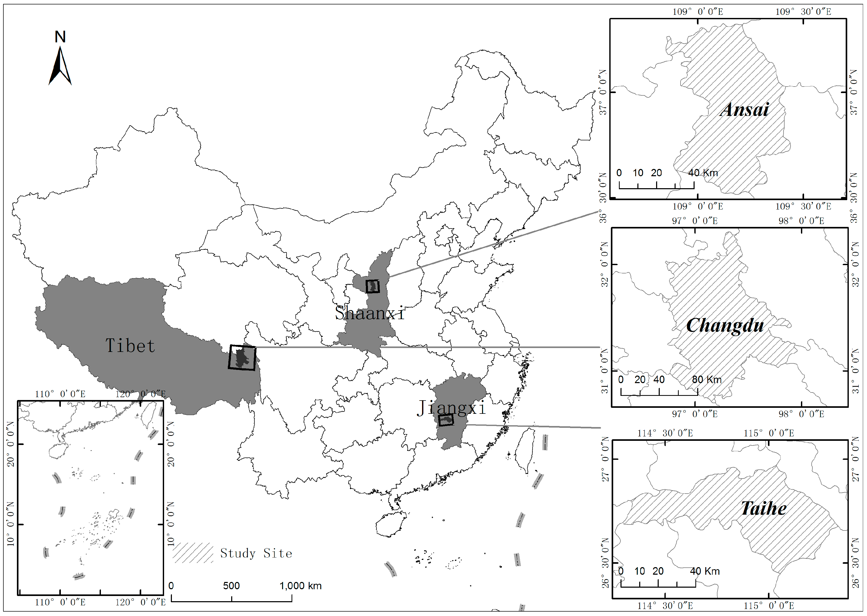
Three study areas in different geographic locations of China were chosen for this study: Taihe County in the Jiangxi Province in the mountainous area of eastern China; Ansai County in the Shaanxi Province in the Loess Plateau in central China; and Changdu County in Tibet, which is located in the Qinhai–Tibet Plateau of western China. The locations of these study sites are shown in
Figure 1.
Taihe County is in the middle southern part of the Jiangxi Province, within 26°27′–26°59′ N and 114°57′–115°20′′ E, and has subtropical monsoon climate. Its annual average temperature is 18.6 °C and the annual average precipitation is 1726 mm. The total area is 2667 km2; high hills account for 5.92% of the total area, low hills make up 54.52%, and plains comprise 27.6%.
Ansai County is located in the north of Shaanxi Province, within 36°31′–37°19 N and 108°6′–109°26′ E, and a total area of 2950 km
2. It has a semiarid monsoon climate, annual average temperature of 8.8 °C, annual average precipitation of 505.3 mm. The vegetation species in this region gradually change northward, from broadleaved deciduous forests to shrub and grassland. This county suffers from severe water loss and soil erosion [
19,
20].
Changdu County is in the east of Tibet, within 30°44′–32°19′ N and 96°42′–97°58′ E, with a total area of 10,652 km2. Its average altitude is more than 3500 m. Affected by the altitude and terrain, it has a plateau subtemperate sub-humid climate. Its annual average temperature varies between 3 °C and 8 °C and the annual average precipitation is 477.7 mm.
2.2. Data
The remote sensing data used in this study are RapidEye L1B imagery with a spatial resolution of 6.5 m. The details of the RapidEye image can be found in
Table 1. It contains blue, green, red, red edge, and infrared bands [
21]. Both red band and near infra-red band are sensitive to vegetation. Because red band is common in both old and latest remote sensing sensors, and some scholars also used it for semivariogram study [
10,
22], the red band is utilized for analysis in this paper.
Table 2 shows some extra information on the images used. There are four raw images for Ansai County, three of which were obtained in September 2010 and one was obtained in October of the same year. Taihe County is also covered by four raw images. They were captured on different dates; one was taken in November 2011, two in September 2012, and the last one in October 2010. For Changdu County, five raw images are available, but only the two images that cover the majority of this region with good quality were used in the end, which were captured in September 2010. Due to the low quality of the remaning images, the marginal area in the northern and southeast of Changdu County is not covered in this study. All raw images were orthorectificated and mosaicked into one image before interpretation, which was later cut by the boundary of their corresponding county.
2.3. Semivariogram
There are several types of calculations of semi-variograms in remote sensing; Equation (1) is mostly used [
23].
where
N(h) refers for the total number of pairs of points within a distance
h and
Z(
si) and
Z(
si +
h) are the values at Point
si and Point
si +
h, separated by a distance of
h pixels [
24]. By changing
h, an ordered set of semivariances is obtained, which constitutes the experimental semivariogram [
25].
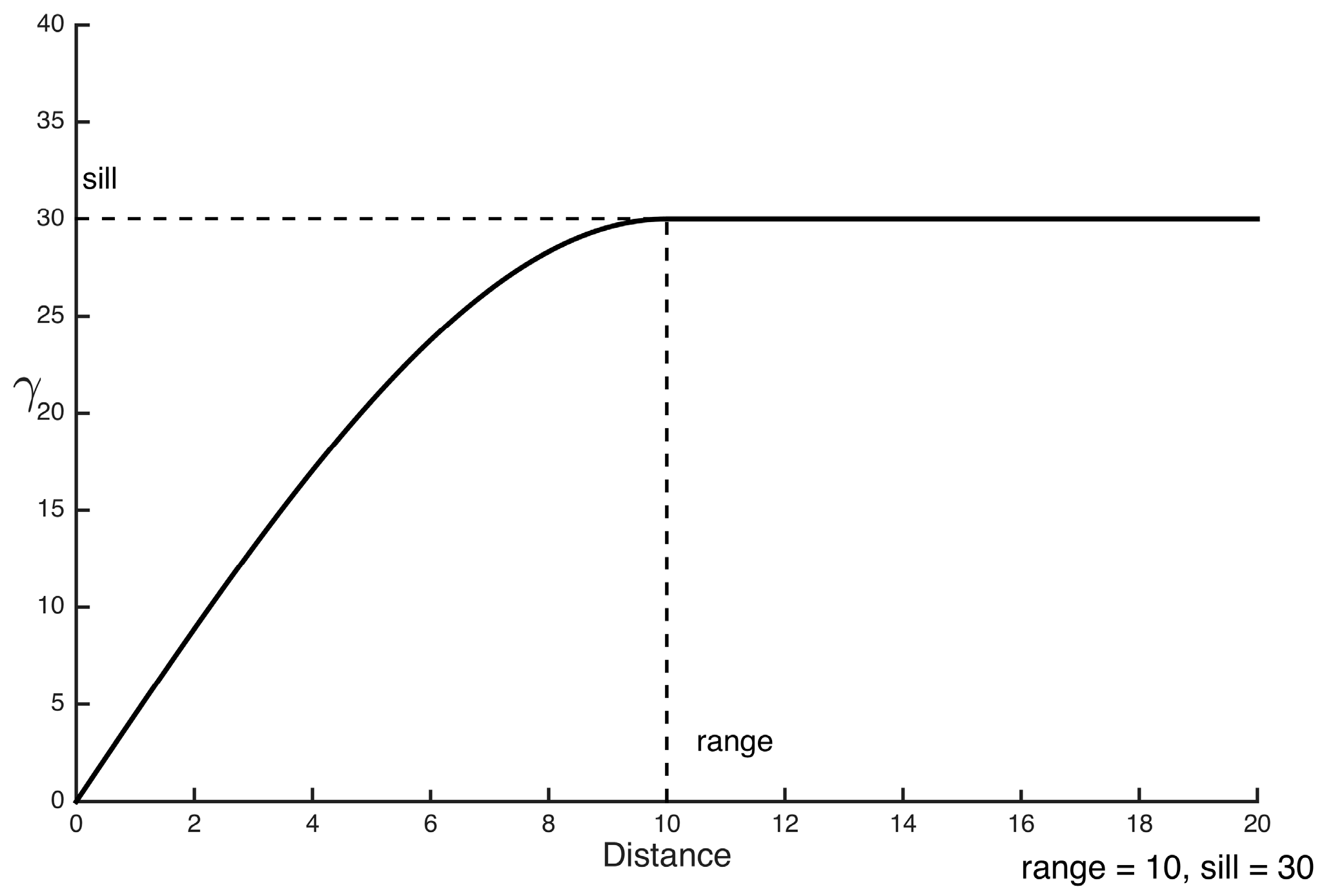
An ideal semivariogram curve is shown in
Figure 2. The assumption in semivariogram theory is that closer objects are more related than distant objects. When the distance between two objects is small, those objects are probably similar or of low variance. In an extreme scenario, when the distance is 0, those two objects are the same. Thus, the variance is zero. As the distance increases, the variance starts to increase. However, when the distance exceeds a specific threshold, the variance reaches its maximum and will no longer change. This threshold is known as
range, indicating the influence scale of an event. In remote sensing, objects are pixels and the
range represents the size of the ground feature. The maximum variance is called
sill, which is an estimator for the true variance of those pixels [
7,
12]. Note that, in this study,
nugget is not considered, and its value is set 0. Forest, grassland, and farmland are assumed to be isotropic.
As the
range was measured in pixel, the real size of the ground feature can be calculated using Equation (2):
where the
range is the value estimated for the
range and
resolution is the size of the pixel, which is 6.5 in this study.
In practice, a serial of parameters should be defined before establishing a semivariogram. Firstly, to build the semivariogram, three parameters are needed, namely, the sample size (SS), maximum distance (MD), and group number (GN). The sample size refers to the number of randomly selected pixels within an image; all distances between pixels will be calculated. The maximum distance defines the radius of a circular area; all pixels outside of this area will be excluded from the calculation. The group number is the number of groups which the distances (from zero to maximum distance) are divided into. Then, to obtain its attributes, range and sill, a model is needed to fit the semivariogram curve. The most widely used models are the linear, spherical, and exponential models.
2.4. Data Processing
The workflow in this study is shown in
Figure 3. It includes three data processing sessions: (1) image interpretation; (2) method comparison; and (3) parameter optimization.
Image interpretation: In this session, an object-based automatic classification method, as well as the manual visual interpretation (manually identifying ground features according to prior knowledge on them, such as feature’s shape, size, pattern, tone, and texture), was used to identify farmland, built area, water, barren, grassland, and forest from remotely sensed images in eCognition software with its multiresolution segmentation algorithm [
26]. First, some ground features such as farmland, built area, and water were visually interpreted, as they either mix easily with other adjacent ground features, such as farmland, or are hard to maintain their shape in the image segmentation, such as river (included in water). By doing this before the image segmentation, the shapes of those ground features could be maintained and high classification accuracy could be ensured. Image was segmented with a scale parameter (SP) of 200 into unclassified objects, and then those objects were classified based on different indexes, such as normalized difference soil index (NDSI), digital number (DN), normalized difference vegetation index (NDVI), brightness, and normalized difference water index (NDWI). The indexes and their value used for a specific ground feature could be found in
Table 3. The value for those indexes were optimized through incremental adjustment to get the best result. Note that, the ground features in those counties were identified in the specific order listed in
Table 3, and the order should not be changed, otherwise, different results may be derived. For accuracy assessment, a number of random points were generated, and Google Earth was adopted to check the points one by one manually.
Method comparison: The proposed MCS-based approach was compared with the sub-area method (SAM) and direct-analysis method (DAM) by applying them to the same area. A pilot area in Ansai County was selected to conduct the method comparison.
The SAM approach randomly selects 30 sample points for each ground feature (e.g., forest and grassland) using a stratified random sampling method based on land cover map. A rectangular area with a size of 500 by 500 pixels around each sample point was then created, which was called sub-area and used to extract subimage from the raw image. Those subimages in SAM are square and only cover a portion of a ground feature, they are then analyzed and the average of their estimated ranges will be calculated. Note that land cover map is not a must for SAM, subimages may be manually extracted from the raw image without land cover map and just based on individual’s judgement. However, this study used land cover map to improve efficiency of this step by automating this process.
The raw image was divided into five subimages based on the land cover map in the DAM. Therefore, there is one image for each ground feature. Different from the regular square subimages in SAM, the subimages in DAM were much larger, covering the entire area of a ground feature, and of irregular shapes. The images of different ground features are analyzed individually.
The MCS approach is built on the DAM. Instead of one-time analysis, MCS runs the analysis multi times to obtain a number of parallel estimations of the range. Monte Carlo methods are a broad class of computational algorithms that rely on repeated random sampling to obtain numerical results [
27]. One significant feature of this method is the large quantity of repetitions. Here, each simulation outputs a value for the estimated
range and the average of all fitted ranges is considered to be the estimator of the true range. MATLAB equipped with a parallel-computing toolbox [
28,
29] was used to shorten the processing time by running several analyses simultaneously.
Parameter optimization: The semivariogram parameters, namely, the sample size (SS), maximum distance (MD), and group number (GN), as well as the model and the simulation number, are to be optimized one by one through four assessment rounds.
To make the data processing procedure more efficient, Python was introduced as a script language for ArcGIS to conduct batch processes such as image separation and random points generation. In addition, a customized function was developed to generate rectangular areas with assigned sizes (width and height), which were used to extract subimages from the raw image.
5. Discussion
5.1. Comparison of Semi-Variogram-Based Methods
The SAM is a development of the inefficient manual process of choosing sub-area images. By controlling the amount and size of subimages, the estimation accuracy of the ranges can be guaranteed and the data size can be minimized. The advantage of SAM is that the estimation is unbiased and reliable because all pixels of a subimage are used to construct the semivariogram. The drawback is that if a random point generated by the stratified random sampling method happens to be close to or on the boundary, the subimage derived from it will probably cross the boundary and contain pixels from other feature classes, which lead to an estimation bias.
The DAM deals with the disadvantages of SAM. In DAM, feature classes are completely separated from each other and semivariogram analysis is conducted. Thus, each subimage can be treated as simple scene. However, if the image size is overly large due to a large survey area, this method is limited by the computing and memory capacities of the computer and the number of pixels needs to be controlled. As a result, only a part of the pixels can be used to construct the semivariogram, which may lead to an estimation bias.
The MCS is a DAM upgrade. Basically, it increases the number of simulations, from DAM’s mere one simulation to many simulations. This helps to overcome the drawback of DAM and avoid the potential biased result. Meanwhile, it utilizes the advantage of DAM with respect to eliminating or minimizing the influence of neighboring feature classes. Furthermore, this method does not depend as much on the capacity of the computer. By adjusting the sample size and amount of simulations, MCS can obtain a reliable estimation of the range. Due to its flexibility, the MCS approach is suitable for this study.
5.2. Impact of Parameters on the Semivariogram
The parameters (i.e., GN, SS and MD), model, and number of simulation have notable influences on the outputs. The preliminary comparison between the outputs before and after parameter optimization shows that the ranges of all three ground features have a lower variance after optimization. Therefore, parameter optimization is necessary. (1) For GN, a larger value is not recommended because it might incorporate too many details, which would consequently reduce the fitting quality. This study suggests that the GN should be controlled at <50. (2) SS is the actual number of pixels used for the analysis. Based on more samples, the output is supposed to be more reliable. This study reveals that there may exist a threshold for SS, after which, the accuracy would only vary slightly, such as farmland in Ansai County, grassland in Taihe County, and farmland in Changdu County. These thresholds could be used as optimized values for SS. However, in most cases, as restricted by the capacity of the computer, the sample size cannot be extended large enough in experiment to identify the threshold. In this scenario, the maximum sample size the computer can handle should be identified and applied to subsequent research. (3) The model selected affects the fitting accuracy. The general criterion for an ideal model is a relatively high R2. In this study, the exponential model outperforms the spherical model. (4) The MD is the most difficult parameter to control. Theoretically, the MD should be large enough to reflect the true range. To obtain a qualified value for MD, two factors need to be considered, namely, the true range and to what extent the MD should exceed the true range. While the true range can be roughly estimated using initial tests, the second factor is the real problem. In this study, three times the average range derived in the parameter optimization session is used as the recommended value to make sure it is large enough to reflect the true range. This is a rough estimate and needs to be further studied.
The authors made those recommendations mainly based on the tremendous amount of calculations and the consequent relationship between parameters and fitting R2. Even though some of the parameters, such as GN, cannot be clearly defined as optimized, the influence of those parameters on the accuracy of semivariogram has be well revealed, based on which, better decisions could be made on setting the parameter for semivariogram than before.
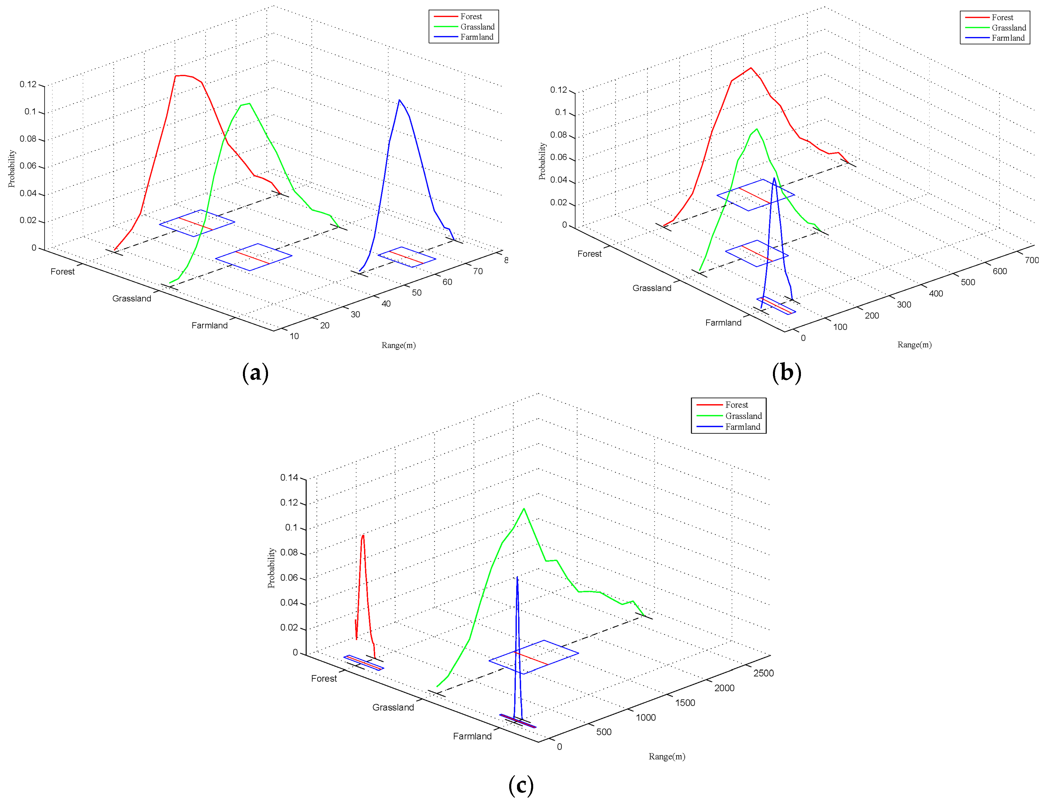
5.3. Differences in the Ground Feature Size in Different Regions
Figure 12 shows the average ranges for general ground features in each region.
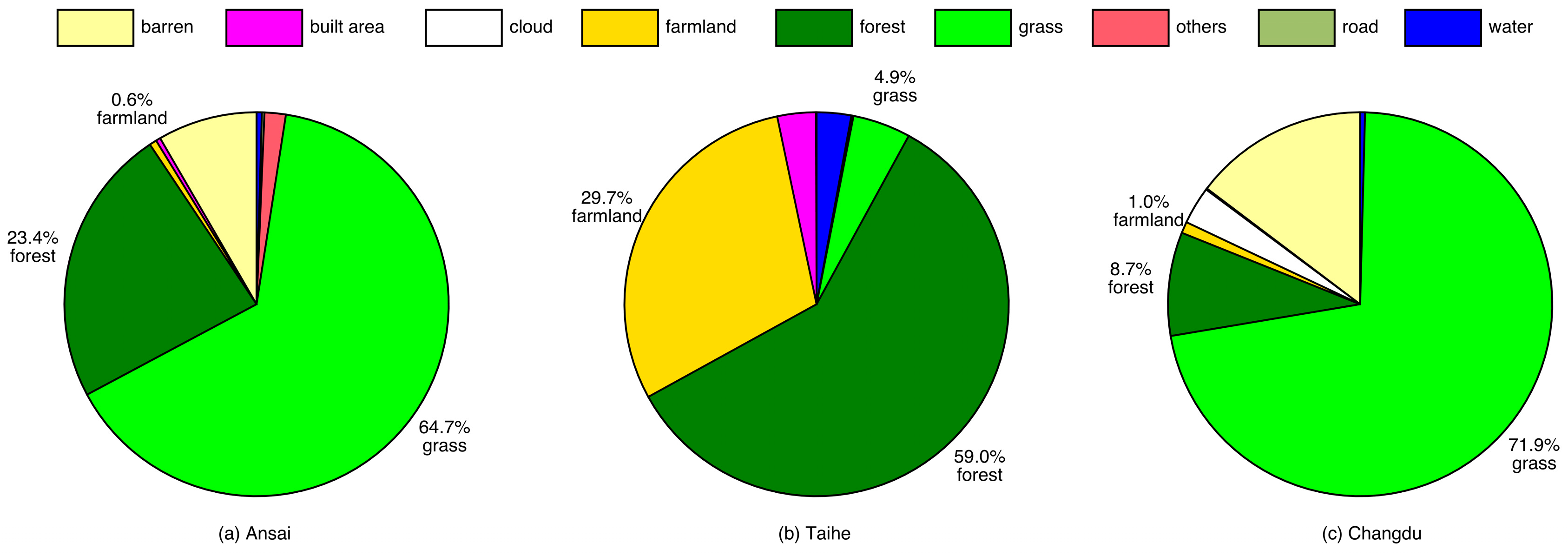
Based on the land cover map of each region, the area for each ground feature was calculated; the percentage is shown in
Figure 13.
Grassland is dominant in Ansai County, accounting for 64.7% of the total area. Forest accounts for 23.4% and farmland for only 0.6%, as shown in
Figure 13a. Grassland comprises the largest area in this region, but its estimated range is the smallest among the three regions, only 45 m, indicating that the grassland in Ansai is fragmentized. This may be explained by severe soil loss in that region [
20], which results in the grassland being cut into pieces. Farmland covers the smallest area but the largest estimated range in this region, reaching 63 m, which means that the farmland is more concentrated than the other two ground features in Ansai. The reason is mainly that most farmland has to be concentrated and distributed along the river for easier irrigation because of lacking water in this area [
20].
Forest is the primary ground feature in Taihe County, accounting for up to 59.0%. Grassland comprises only 4.9%, while farmland covers 29.7% of the total area, as shown in
Figure 13b. The forest occupies the largest area in this region and the largest average range of 433 m among those regions, indicating that forest is widely and continuously distributed in Taihe County. This matches the real situation well. Taihe County is located in the southeast of China where there is abundant water and large forests [
30]. The relatively small average range for farmland shows that the farmland is dispersed. East China has a large population, which leads to a high demand on food supply. Much of the land has been reclaimed for food production, which is why the farmland has a higher proportion than the other two counties. However, the farmland is separated by hills, which makes the farmland relatively small [
31].
Changdu County is located in the Qinghai–Tibet Plateau with extensive land and a small population. The landscape there is simple. Grassland accounts for 71.9%, forest occupies 8.7%, and farmland contributes to only 1.0% (
Figure 13c). The grassland area in Changdu County is large and continuous [
32]; therefore, the estimated range is also large, reaching 1308 m. The ranges for forest and farmland are similar; both are ~100 m, which is close to the real situation.
The scale features of ground features acquired using the proposed method for the three representative counties of China could match well with the real local landscape characteristics, which indicates that the proposed method could achieve more than other relevant quantitative studies. In terms of study in other regions, Wen obtained the size of farmland, 98.5 m, for the Sanjiang Plain in Northeast China [
33]. Yang reported that 30 m is an appropriate scale for depicting built area, while 90 m for water in Baoji City in the Loess Plateau [
34]. However, these studies lack description and explanation regarding simulation accuracy, and only focus on one single region, i.e. no comparison was conducted between different regions, which limits its universal application. This study demonstrates the advantage of MCS on directly revealing the size characteristics of ground features in different geographical regions, and has the potential to receive wide popularity.
5.4. Ground Feature Size and Optimal Resolution
The ground feature size is mainly confined within two dimensions in this study and can be considered as an abstract representation of its real size. It is not real because the size of an object in the real world should be characterized based on at least two aspects, length and width, while the “size” calculated from the estimated range of the semivariogram is just a measure of the length. The optimal resolution of an image for the ground feature should be smaller than that size to retain information about that object. The finer the resolution is, the more detail is included in the imagery.
According to Woodcock, variation at a scale finer than the scale of regularization (resolution) cannot be detected and variations less than two to three times the scale of regularization (resolution) cannot be reliably characterized [
7]. Therefore, the optimal resolution for a ground feature should be, at most, one-third the size of that feature, for the variation within it to be reliably detected.
Table 7 recommends the maximum applicable satellite imagery for survey of general ground features in those three counties, based on the maximum resolution that is one-third of average size of ground feature. For example, it could be inferred that the Sentinel-2A imagery with a resolution of 10 m could be used to survey all three areas, and Landsat 8 imagery (15 m) could meet the requirement of almost all areas, except the grassland in Ansai County, while CBERS-2 with a resolution of 20 m could be used to survey most of the areas. Apart from those listed in
Table 7, many commercial satellite imageries provide a resolution less than 10 m that could also be leveraged, such as WorldView-4 (0.31 m), GeoEye-1 (0.46 m), Pleiades-1A (0.5 m), KOMPSAT-3A (0.55 m), QuickBird (0.65 m), Gaofen-2 (0.8 m), TripleSat (0.8 m), IKONOS (0.82 m), SPOT-6 (1.5 m), SPOT-7 (1.5 m), ALOS (2.5 m), CARTOSAT-1 (2.5 m), SPOT-5 (2.5–5 m), and Dove Satellite (3 m) [
35].
6. Conclusions
This study uses MCS to improve the performance of semivariograms by optimizing its parameters, for selecting remote sensing imagery with an appropriate resolution for natural resource surveys. The main contribution of this paper is revealing the relationship between semivariogram parameters and simulation accuracy, as well as the suggestions given on selecting appropriate values for parameters. Apart from that, the sizes of those common ground features in three counties of China are acquired, and satellite image for survey is recommended, which is more objective than the usual subjective way of selecting datasets by experience. The main findings include:
- (1)
-
The proposed MCS performs better than SAM and DAM in determining the ground feature size from large remote sensing imagery by providing more accurate and precise estimations.
- (2)
-
Optimizing the parameters for building and fitting semivariograms is necessary and strongly recommended by the authors because they greatly affect the performance of semivariograms in terms of precision and accuracy. The optimized parameters could improve the precision of the estimations. A larger SS and larger number of simulations is recommended, while the GN should not be too large.
- (3)
-
The size and corresponding optimal resolution for specific ground feature could be acquired using the proposed MCS and the optimized parameters. In this study, three counties in China were used as case study, and appropriate remote sensing image was recommended.
- (4)
-
The sizes of the same ground feature in different regions vary; the sizes of different ground features in the same region also vary. That means the result is specific to a certain area. Nevertheless, the proposed method can also be used for choosing the remote sensing imagery resolution in other places.
There still exists some limitation which should be studied further. First, the influence of the classification accuracy on the estimation has not been studied in this research because the overall accuracies for the three regions are almost identical. The relation between the classification and estimation accuracies is still unclear and needs to be further investigated. In addition, high performance computing (HPC) could be introduced in the future study, and cost–benefit analysis would be incorporated to assess the cost and benefit of this method, to further improve its efficiency.


