There are renewed calls and growing evidence that hypothesis testing should be conducted at the level of significance chosen in consideration of the information specific to the problem under question.
Kim and Ji (
2015) demonstrate how
Leamer’s (
1978) method can be applied to empirical research in finance for more credible significance testing.
Perez and Pericchi (
2014) propose a calibration formula for the adaptive level of significance in the context of simple hypothesis testing, derived as a compromise between Bayesian and non-Bayesian methods.
Pericchi and Pereira (
2016) propose a general approach to determining the adaptive significance level by minimizing a weighted sum of Type I and II error probabilities, showing that their approach is closely related with the inference based on the Bayes ratio. In this section, we use the method based on
Leamer’s (
1978) line of enlightened judgement for the ADF and DF–GLS tests, which is a special case of the general approach of
Pericchi and Pereira (
2016). We present decision-based significance levels for these unit root tests under a range of sample sizes widely encountered in practice. We also examine the effects of other factors (prior probability, relative loss, starting values of the series) that can influence the choice of the decision-based level.
2.1. Decision-Theoretic Approach to Unit Root Testing
In this paper, we propose a decision-theoretic approach to unit root testing. Under this approach, we consider the losses from Type I and II errors of hypothesis testing, and choose the decision that minimizes the expected loss (see, for example,
Arrow 1960;
Leamer 1978;
Das 1994;
Poirier 1995). We observe that empirical researchers often make decisions in a dichotomous and mechanically way, based on an arbitrary threshold set by a conventional level of significance. We are concerned that this practice has rendered many empirical researchers make too rash decisions in favour of a unit root. As a result, there are a number of stylized facts that are not consistent with economic reasoning. For example, while most of economists believe that real exchange rates and interest rates are stationary, a large body of empirical studies report that these time series have a unit root. We argue that these stylized facts, inconsistent with economic reasoning or theories, are the results of conducting unit root tests at a conventional significance level. This point is in line with the concerns raised by the American Statistical Association (
Wasserstein and Lazar 2016), with a statement that “Widespread use of ‘statistical significance’ (generally interpreted as ‘
p < 0.05’) as a license for making a claim that a scientific finding (or implied truth) leads to considerable distortion of the scientific process”.
We note that failure to reject the null hypothesis of a unit root does not necessarily indicate the full support for a unit root. It tells us that we cannot rule out the presence of a unit root, while the alternative hypothesis is also likely. Under the decision-theoretic approach, we consider the expected loss under a range of the key parameters and choose the most likely action. With this approach, the researcher’s prior belief for H
0 and H
1; and relative loss between Type I and II errors play important roles, which are totally ignored in conventional hypothesis testing. If the researcher believes that a unit root is unlikely based on economic reasoning, she should assign a low value to the prior probability for H
0 and/or a low value to the loss of Type I error (relative to that of Type II error). In so doing, the researcher is likely to reject the unit root hypothesis. As we shall see later in our applications, the use of conventional significance level for unit root testing is associated with the case where the researcher a priori believes that the null hypothesis of a unit root is highly likely and/or she assigns a high loss to Type I error (relative to that of Type II error). In many applications (e.g., real exchange rate or interest rates), such prior belief and relative loss values implied by a conventional significance level may not be consistent with economic reasoning. This decision-theoretic approach is also closely related with the Bayesian view of unit root test, where the decision is made based on the posterior odds ratio (see, for example,
Sims 1988;
Sims and Uhlig 1991)
5. The latter compares the posterior probabilities under H
0 and H
1, which aid the decision to choose a more likely hypothesis (see
Startz 2014).
2.2. Line of Enlightened Judgement and Decision-Based Significance Levels
It is well known that a trade-off between the two error probabilities (
α and
β) of hypothesis testing exists, with a higher (lower) value of
α associated with a lower (higher) value of
β. When
α is set at 0.05, a low power means that the value of
β is much higher than 0.05. For example, if the power is as low as 0.20, there is a serious imbalance between
α and
β, with the latter being 16 times higher than the former. As a result, the test is severely biased towards Type II error, with a consequence that a false null hypothesis fails to be rejected. By choosing a higher value of
α in this case, say 0.3, one can achieve a balance between
α and
β, obtaining a higher power at the same time. The line of enlightened judgement (
Leamer 1978) is formulated by plotting the combination of all possible
α and
β values, from which one can choose a desired combination in explicit consideration of the power and losses under Type I and II errors.
In what follows, the line of enlightened judgement for unit root tests is presented. Following
DeJong et al. (
1992), we consider the time series:
where
ut is an independent error term with zero mean and fixed variance
σ2. The standardized initial value of (1) is denoted as
. The model (1) can be re-written in the ADF form as
Taking the ADF test as an example, the test statistic for H
0:
λ = 0; H
1:
λ < 0 is
, where
λ ≡ (
τ − 1) and
. Let
be the least-squares (LS) estimator for
λ and se(
) denote its standard error estimator. Note that
, where
CR(
α) is the
α-level critical value and
. The line of enlightened judgement is obtained by plotting all possible combinations of
α and
β.
A Monte Carlo experiment with the number of trials 10,000 is conducted to calculate the (
α,
β) values, using
MacKinnon’s (
1996) critical values. Following
DeJong et al. (
1992), the data is generated from model (2) with
p = 2,
ρ1 = 0.5,
δ0 =
δ1 = 0, setting
λ =
λ1, where
λ1 is a value of
λ under H
1. In evaluating the power of the test, the choice of the value of
λ1 is important: in this study, we are guided by a past seminal study.
6 According to
DeJong et al. (
1992),
λ1 ∊ [−0.15, 0] is a plausible range of the parameter values under H
1. In particular, they recommend
λ1 = −0.15 for annual time series and
λ1 = −0.05 and −0.01 for quarterly and monthly data, respectively. From a grid of
α values between 0.01 and 0.99 with an increment of 0.02, the proportion of Type II error is obtained as an estimate of
β. The standardized initial value
X0* is set initially at 1.5, which is the most plausible value according to
DeJong et al. (
1992).
7We also present the line of enlightened judgement for the DF–GLS test of
Elliott et al. (
1996), which is well known to have a higher power when the initial value is small. The test involves a simple modification to the ADF test by de-trending the deterministic component using the GLS method. For the ADF and DF–GLS tests (for the model with a constant only), the lines of enlightened judgement are constructed using appropriate
MacKinnon’s (
1996) critical values. For the model with a constant and a linear trend, the DF–GLS test statistic follows a limiting distribution different from that of the ADF. For this case, we use the critical values from the asymptotic distribution of the test statistic obtained by simulation following
Elliott et al. (
1996).
8According to
Leamer (
1978), the expected loss from hypothesis testing is
pαL1 + (1 −
p)
βL2, where
p ≡
P(H
0),
L1 represents the loss of Type I error and
L2 that from the Type II error. Given the combinations of (
α,
β) values on the line of enlightened judgement, the level of significance
α* can be chosen so that the expected loss is minimized. The value of Type II error probability corresponding to
α* is denoted as
β*. The specific values of
p,
L1 and
L2 depend on contexts and the researcher’s prior belief. For the purpose of simplicity, we initially assume that
p = 0.5 and
L1 =
L2, by which the minimization of the expected loss is simplified to that of
α +
β. These assumptions mean that the researcher gives an equal weight to the two states of nature (H
0 and H
1) with a prior belief that: firstly, they are equally likely to be true, and, secondly, the losses from Type I and II errors are identical. In the analysis that follows, we will allow for general values of
p and
L’s. In this paper,
α* is referred to as the decision-based significance level.
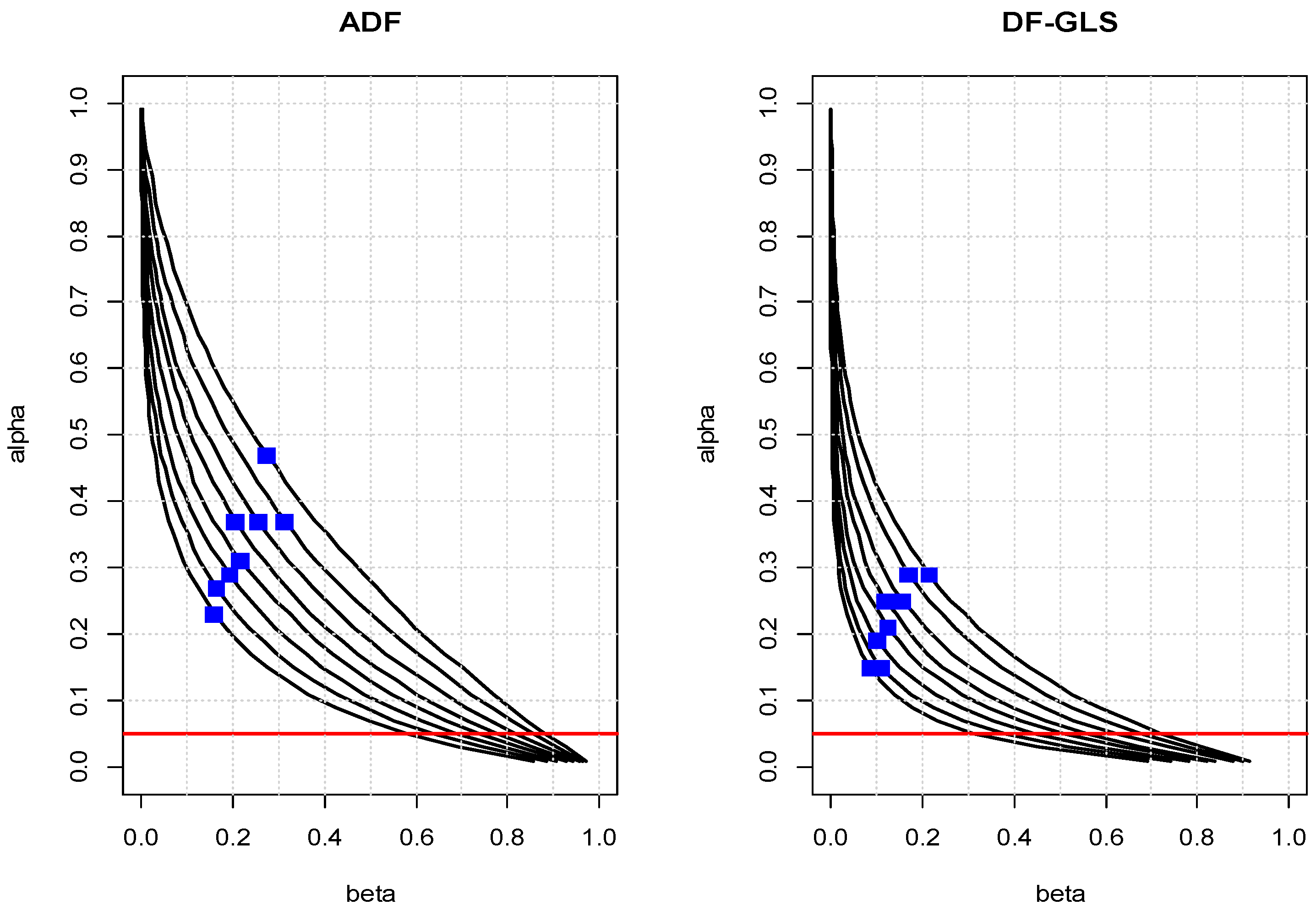
Figure 1 presents the lines of enlightened judgement for the ADF and DF–GLS tests for the model with a constant and a linear trend, when
λ1 = −0.15, under the sample sizes ranging from 60 to 130. These settings are suitable for annual time series. The line shifts towards the origin as the sample size increases, corresponding to lower values of
β (or higher power) for a given value of
α. The blue square dots represent the points of (
α*,
β*), where the expected loss (
α +
β) is minimized. The decision-based significance levels of the DF–GLS test are much lower than those of the ADF test due to its higher power. For all sample sizes, they are in the neighborhood of 0.3, except when
n = 60 for the ADF test, which is consistent with
Winer’s (
1962) assertion. They also decrease with the sample size as
Leamer (
1978) suggests. From
Figure 1, when
n = 100 and
α = 0.05,
β = 0.74 and the power of the ADF test is only 0.26: i.e., as mentioned above, a case of low power with an obvious imbalance between
α and
β. However, if
α is chosen to minimize the expected loss (
α +
β), (
α*,
β*) = (0.31, 0.22) with a substantially higher power of 0.78. The expected loss is much higher when
α = 0.05, as expected. The critical value at the decision-based significance level is −2.54, which is much larger than the 5% critical value of −3.46. Similar results are evident for the DF–GLS test.
Table 1 presents complete listing of the values indicated in
Figure 1.
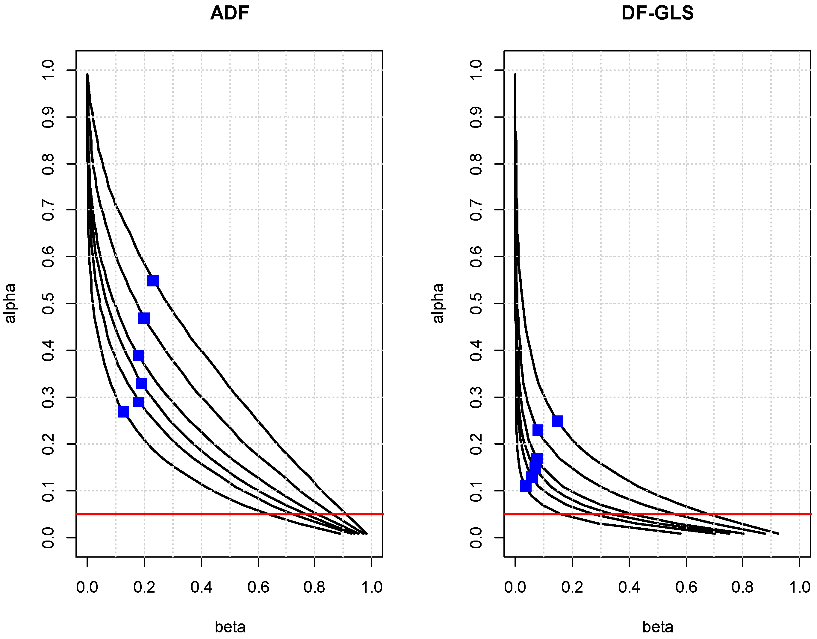
Figure 2 presents the lines of enlightened judgement associated with the ADF and DF–GLS tests for the model with a constant only, when
λ1 = −0.05 for the sample sizes ranging from 80 to 240. These settings are suitable for quarterly time series. Again, higher power associated with the DF–GLS test is evident with the lines for the DF–GLS test much closer to the origin than those of the ADF. When the sample size is 120 and
α = 0.05, the DF–GLS test is again severely biased towards the Type II error, with its
β value more than 11 times higher than that of
α. The power is 0.44, which is much higher than that of the ADF which is 0.13, as expected. However, at the decision-based significance level
α* = 0.23, the DF–GLS test enjoys a substantially higher power of 0.92 with a balance between the two error probabilities. Overall, the decision-based significance levels for the DF–GLS test are in the neighborhood of 0.20 for a typical quarterly time series.
Table 2 presents complete listing of the values indicated in
Figure 2.
From
Figure 1 and
Figure 2, we observe a tendency where the decision-based level (
α*) is more or less twice the size of the corresponding Type II error probability (
β*). This means that the test at the decision-based significance level tends to be conservative about the Type II error, in contrast with the case of
α = 0.05 where the test is severely biased towards Type II error. It should be noted that the conventional levels of significance (such as 0.05) represent a poor benchmark level for these tests because they cannot be optimal under any sample sizes frequently encountered in practice. The level of significance in the 0.2 to 0.4 range may be “outrageously high” in comparison with the 0.05 level as
Arrow (
1960, p. 73) puts it, but the test will enjoy a considerably higher power with a balance between Type I and II error probabilities.
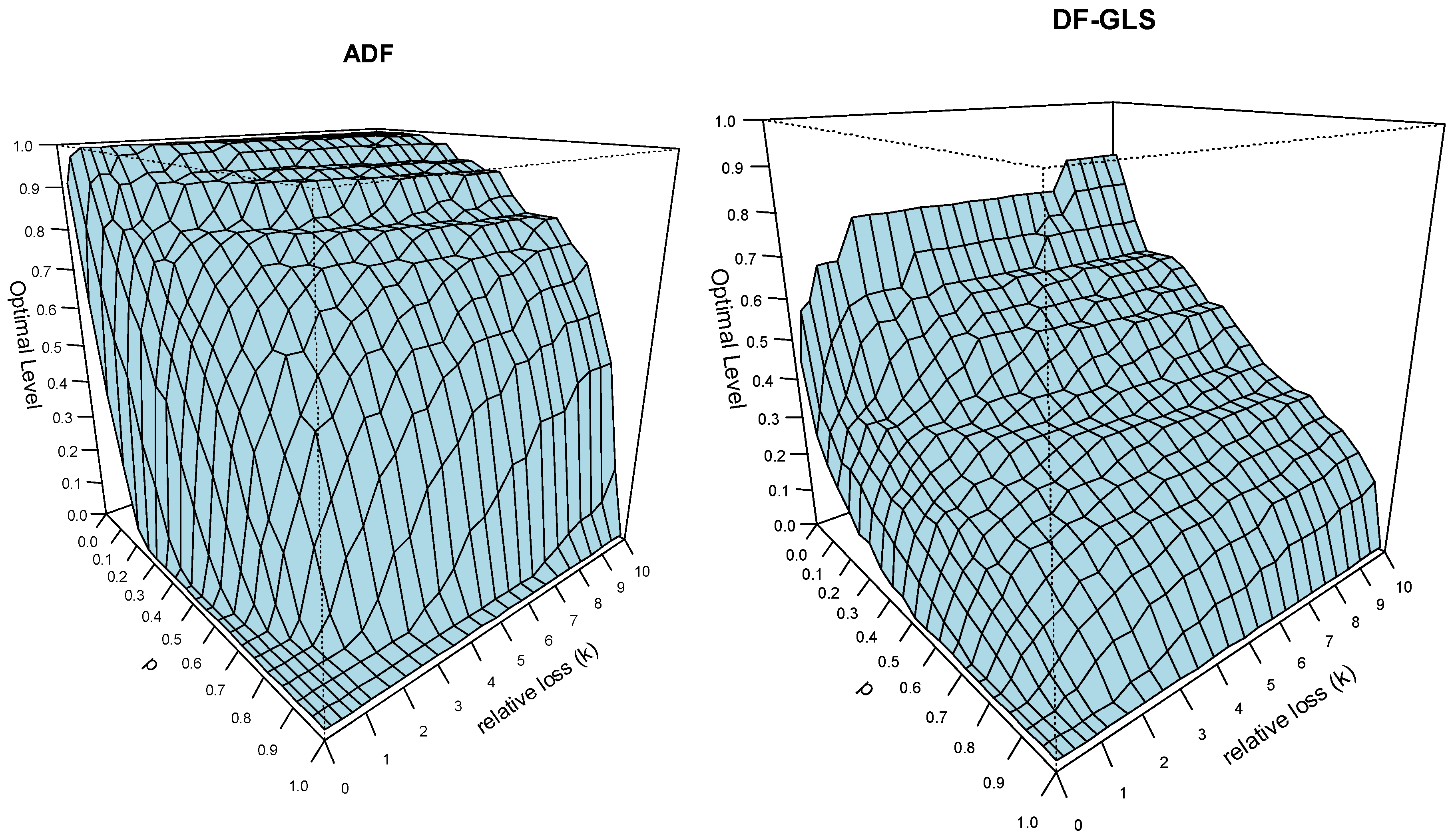
2.3. Factors Affecting the Decision-Based Significance Level
Koop and Steel (
1994, p. 99) consider the lack of formal development of loss function as a serious weakness of both Bayesian and classical unit root studies. They argue that the classical analysis has an implicitly defined loss function in choosing the level of significance, in which losses are asymmetric. That is, the use of a conventional level of significance (such as 0.05) implies an arbitrarily asymmetric loss function. While our analysis so far assumes a symmetric loss function (
L1 =
L2), it is possible that the value of the decision-based level changes in response to different values of relative loss from Type I and II errors. In addition, there are other factors that possibly affect the decision-based level; i.e., the probability for the null hypothesis (
p) that is so far assumed to be 0.5; and the starting value of the series that may affect the power of a unit root test.
To examine the effects of the prior probability for H
0 and the relative loss,
Figure 3 plots the decision-based significance levels for the ADF and DF–GLS tests (model with a constant only) as a function of
p and relative loss. Letting
k =
L2/
L1 (relative loss) and setting
L1 = 1 without loss of generality, the expected loss is expressed as
pα + (1 −
p)
βk. These values are calculated from the lines of enlightened judgement given in
Figure 2 when
n = 120, by minimizing the expected loss
pα + (1 −
p)
βk under different values of
p and
k. It appears that they change sensitively to the value of
p and
k, and that the conventional levels of significance (such as 0.05 and 0.01) are justifiable only when
p is high and
k is low. That is, either when the researcher has a strong prior belief that H
0 is true (presence of a unit root) or when the loss from Type I error considerably outweighs the loss associated with Type II error. In the opposite case, the decision-based level can often be far higher than 0.50 for both tests. Under moderate values of
p and
k, the decision-based levels are in the 0.2 to 0.4 range.
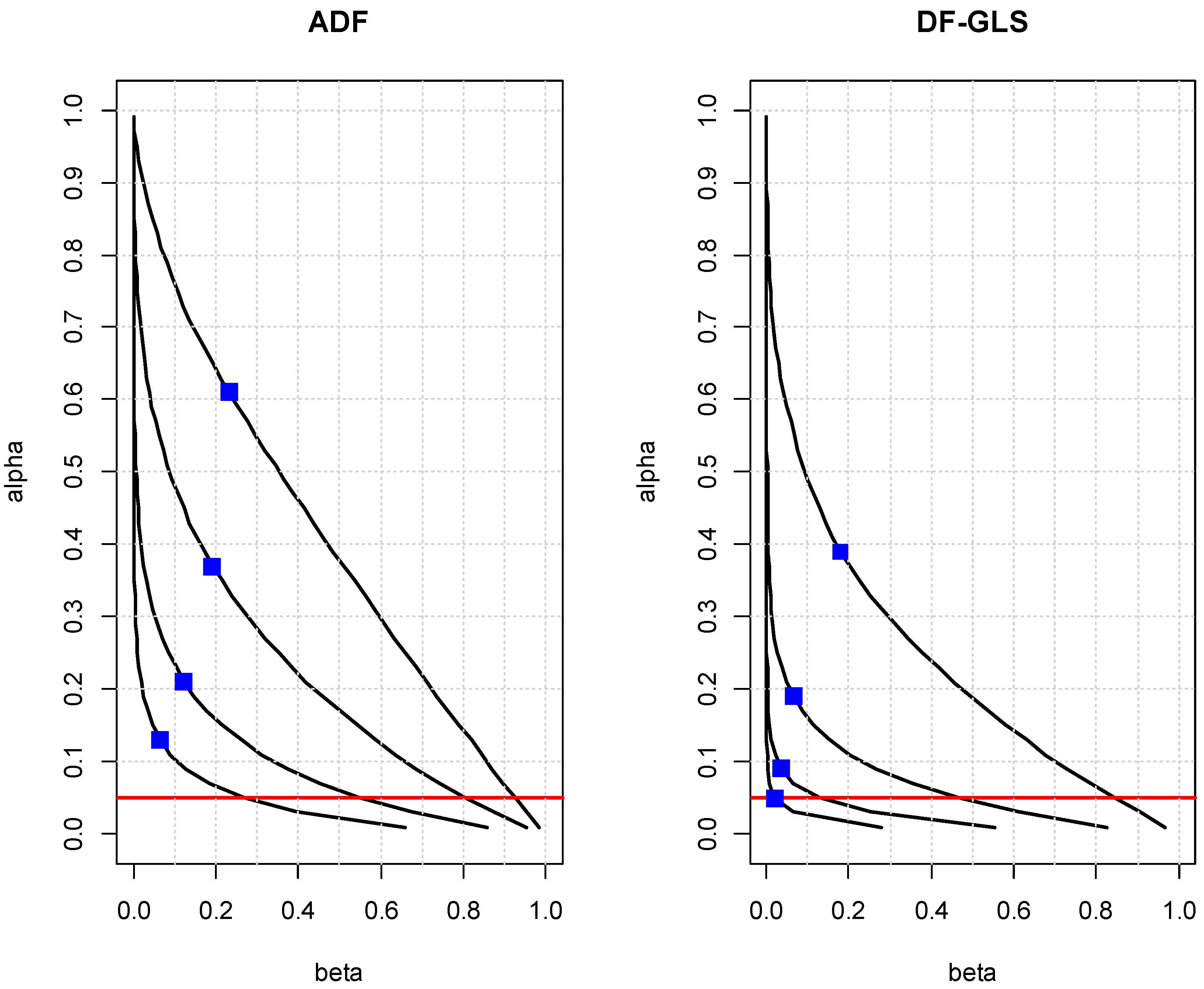
It is well known that the power of unit root test changes sensitively to the initial value and the degree of autocorrelation of the error term (see
DeJong et al. 1992;
Müller and Elliott 2003). To examine the sensitivity, the decision-based levels of significance for the ADF and DF–GLS tests (model with a constant only) are reported in
Table 3 when
n = 120, under a range of
X0* and
ρ1. For the ADF test, under a reasonable value of
X0* (0 to 5), it appears that the decision-based level of significance is not sensitive to
ρ1. For the DF–GLS test, it changes sensitively, especially when the value of
ρ1 is negative, and tends to increase with the starting value. The decision-based level’s sensitivity to the values of
p and
k and the starting value of the series are taken into account in the calibration rules that will be discussed in the following section.


