Görtler Vortices in the Shock Wave/Boundary-Layer Interaction Induced by Curved Swept Compression Ramp

Abstract

This study builds on previous research into the basic flow structure of a separated curved swept compression ramp shock wave/turbulence boundary layer interaction (CSCR-SWBLI) at the leading edge of an inward-turning inlet. We employ the ice-cluster-based planar laser scattering (IC-PLS) technique, which integrates multiple observation directions and positions, to experimentally investigate a physical model with typical parameter states at a freestream Mach number of 2.85. This study captures the fine structure of some sections of the flow field and identifies the presence of Görtler vortices (GVs) in the CSCR-SWBLI. It is observed that due to the characteristics of variable sweep angle, variable intensity interaction, and centrifugal force, GVs exhibit strong three-dimensional characteristics in the curved section. Additionally, their position is not fixed in the spanwise direction, demonstrating strong intermittence. As the vortices develop downstream, their size gradually increases while the number decreases, always corresponding to the local boundary layer thickness. When considering the effects of coupling of bilateral walls, it is noted that the main difference between double-sided coupling and single-sided uncoupling conditions is the presence of a large-scale vortex in the central plane and an odd number of GVs in the double-sided model. Finally, the existence of GVs in CSCR-SWBLI is verified through the classical determine criteria Görtler number (G_T) and Floryan number (F) decision basis.

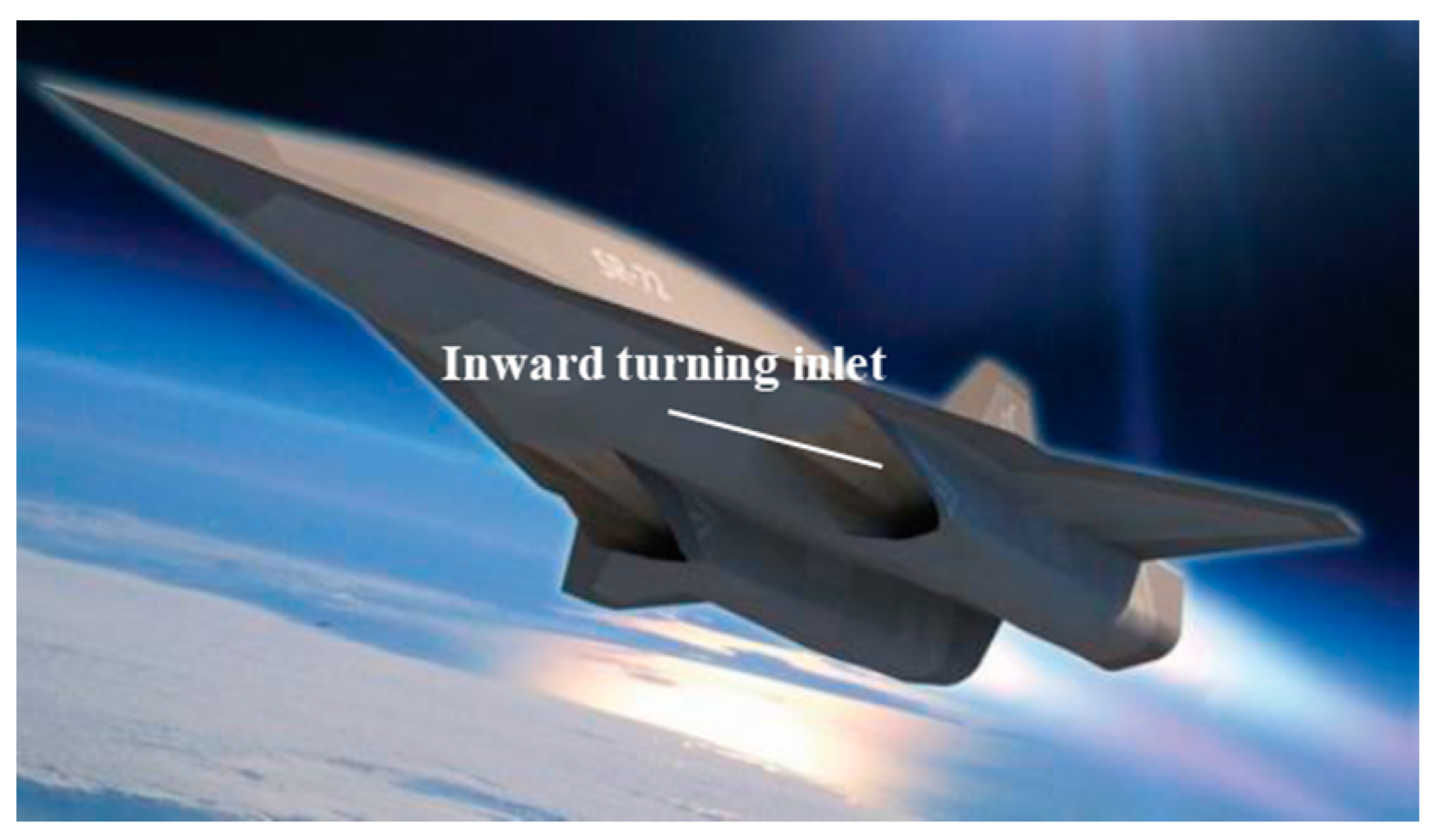
1. Introduction

The inlet, situated at the front of the air-breathing propulsion system, captures incoming flow and supplies the engine with low-speed, high-pressure airflow. It significantly influences engine efficiency, flight envelope, and operational safety [1]. As inlet aerodynamic technology advances, researchers have turned their attention to the three-dimensional inward-turning inlet, which is highly integrated with the fuselage and designs based on the streamline-traced method [2,3,4,5,6,7], as shown in Figure 1. Numerical results show that compared with traditional two-dimensional and axisymmetric inlets, the inward-turning inlet has significant advantages in compression efficiency and mass flow capture ability under the same incoming flow conditions and constraints [3,8].

In practical applications, the inward-turning inlet integrated with the fuselage’s forebody often experiences shock wave/boundary layer interaction caused by the external compression ramp-induced shock wave and the body boundary layer [9,10]. Studies on ramp-induced shock and boundary layer interactions primarily focus on compression-ramp SWBLI (CR-SWBLI) [11,12,13,14,15,16,17] and swept-compression-ramp SWBLI (SCR-SWBLI) [18,19,20,21,22,23]. The curved swept compression ramp SWBLI (CSCR-SWBLI) induced by the inward-turning inlet’s compression surface, based on the streamline-traced design methodology, is essentially a CR-SWBLI with variable sweep angle, variable intensity, and distinct three-dimensional characteristics. Notably, its inward compression surface facilitates the formation of complex streamwise vortex structures known as Görtler vortices (GVs) [24]. GVs are large-scale streamwise vortex structures generated by the centrifugal force instability of the airflow on the concave surface, and are always characterized by pairs occurrence and reverse rotation [24]. In recent decades, as research methods have matured, there has been increased understanding of these large-scale vortex structures occurring in compressible high-speed flows. In supersonic/hypersonic flow fields, apart from the extensive and detailed studies on concave ramps [25,26,27] and compression ramps [17,28], researchers have also observed this stripe vortex structures in incident SWBLI (I-SWBLI) [29]. Pasquariello [30] employed LES to discover and define the GV structure in I-SWBLI for the first time. Zhuang [31] confirmed the actual existence of GVs in this flow field using the PLS experimental technique, and Li [32] observed GVs in dual-I-SWBLI. In supersonic air-breathing propulsion systems, GVs can be utilized as a noninvasive mixing technology to induce the required mixing within downstream combustion chambers without incurring total pressure loss [33]. References [34,35] reported that GVs remove low-momentum fluid from near walls by altering local density and pressure gradients in the boundary layer. The mixing ability of GVs is demonstrated by redirecting high-momentum fluid towards the near wall in alternating directional positions. In essence, the mixing capability of GVs also indicates their role in flow transition. The contributions of GVs to flow transition in hypersonic conditions have been verified by both Ren [36,37] and Roghelia [38]. The post-transition boundary layer enhances the stability of the internal flow in supersonic inlets. Moreover, the ability of GVs to mix the mainstream with the boundary layer can improve the uniformity of the inlet internal flow field. Given the significant benefits of GVs for the internal flow field of inlets, this study examines the structural and behavioral characteristics of GVs. This investigation aims to provide novel research insights for inlet designers concerning the control and development of the boundary layer within the inlet fuselage.

In previous experimental and simulation investigations of the separated CSCR-SWBLI, although the author’s team obtained the time-averaged wall pressure distributions characteristics and flow separation topology, they did not find explicit streamwise vortex structures in the time-averaged flow field [39]. In this paper, the transient fine structure of the flow field will be captured to investigate the occurrence of flow vortex structures in the three-dimensional SWBLI using the ice-cluster-based planar laser scattering (IC-PLS) method, which combines multiple observation directions and positions. We will investigate its three-dimensional characteristics and development rules.

2. Methodology

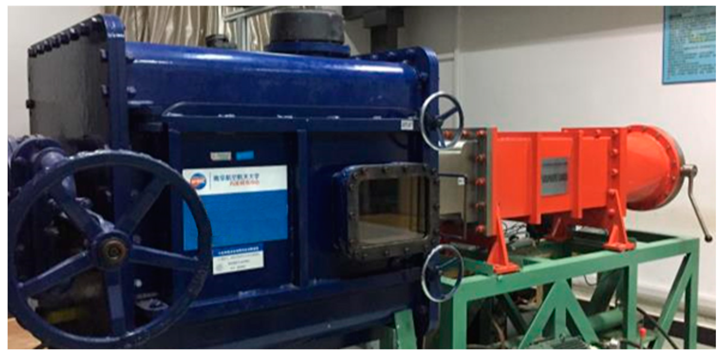
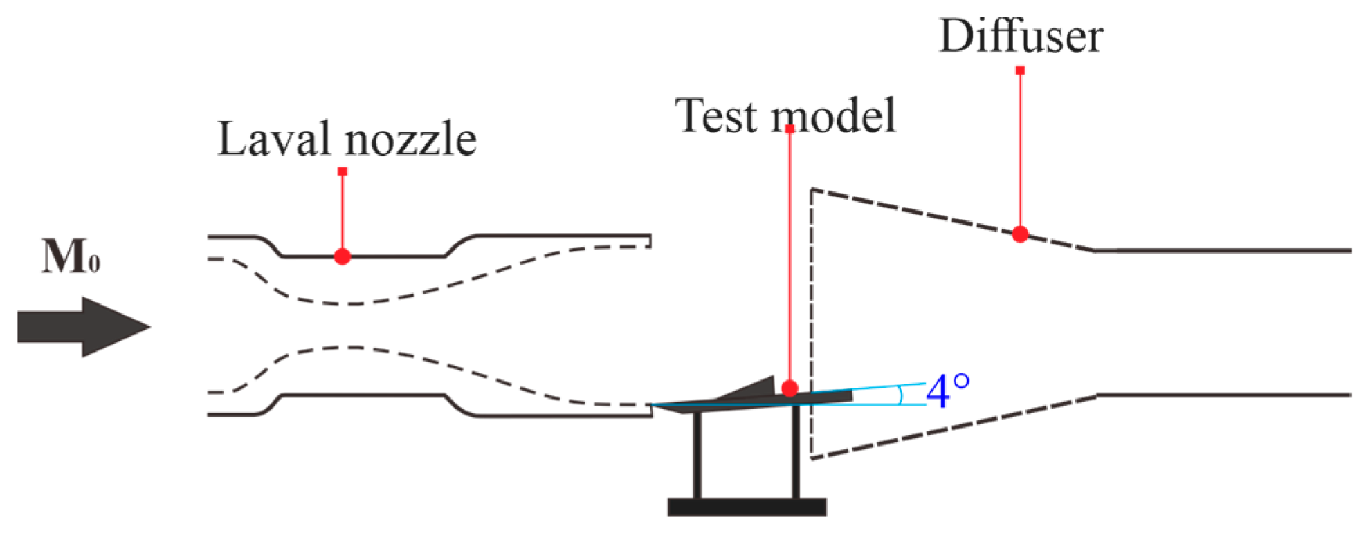
2.1. Description of the Test Model

To isolate and analyze the CSCR-SWBLI phenomenon in the integrated inward-turning inlet design, this study applies a streamline-traced design methodology similar to that used in the inward-turning inlet design. The process involves two primary steps: First, an axisymmetric basic flow field is established based on the design conditions. Next, the inviscid compression surface of the inlet is determined by tracing the frontier capture tube (FCT) at the entrance of the given inlet within the axisymmetric inner cone flow field. As depicted in Figure 2, the incident conical shock wave surface is reflected by the center body, forming a reflection conical shock wave surface and creating the axisymmetric conical basic flow field. Subsequently, a simplified physical model of the inward-turning inlet is derived from the rectangular FCT. Following the principles and physical interpretations described extensively in ref. [40], and taking into account the incoming flow conditions and scale of the wind tunnel, a specific set of physical parameters is determined for typical conditions.

Table 1. Main parameters of streamline tracing technique [40].

Parameters	Value
R, mm	150
r, mm	25
Wc, mm	100
Hc, mm	40
Ec, mm	80
η, deg	11

provides a comprehensive list of the relevant basic cone flow field parameters and inlet capture profile parameters, where R and r represent the outer and inner diameters of the relevant basic conical flow field, W_c and H_c represent the width and height of the capture profile, E_c represents the eccentricity of the capture profile relative to the centerline of the reference flow field, and η is the inner cone angle of the reference flow field.

This paper specifically focuses on the flow field at the junction between the compression surface of the inward-turning inlet and the fuselage’s forebody. To appropriately simplify the physical model, abstraction is necessary. Considering the complexity of SWBLI phenomena, the research is conducted in two steps: first, investigating the uncoupled interference in the single-sided model, and then examining the coupled interference in the double-sided model. It is important to note that the single-sided model specifically addresses the CSCR-SWBLI phenomenon in the curved swept segment. In order to reveal coupling interference from the bilateral wall to the central plane, only half of the double-sided coupling model is utilized, with a certain length extended along the spanwise direction based on its centerline to eliminate sidewall interference in the extended segment. The curved swept segment has a spanwise width of W = 50 mm, and the actual compression angle of the center plane is α = 13.76°, The length of the compression corner’s leading edge from the model’s foremost point is set to 80 mm in order to minimize potential interference from Mach waves. Additionally, a length of 100 mm is chosen for the rear step at the end of the ramp to ensure that it does not impact the upstream SWBLI region along the flow direction. The final experimental model, depicted in Figure 3a (single-sided model) and Figure 3b (double-sided model), comprises a plate, a side observation window with K9 glass (exclusive to the single-sided model), a side wall, and a compression surface. As the picture shows, the leading edge of the plate is flush with the lower surface of the nozzle, and the incoming boundary layer is the fully developed boundary layer on the lower wall of the nozzle during testing.

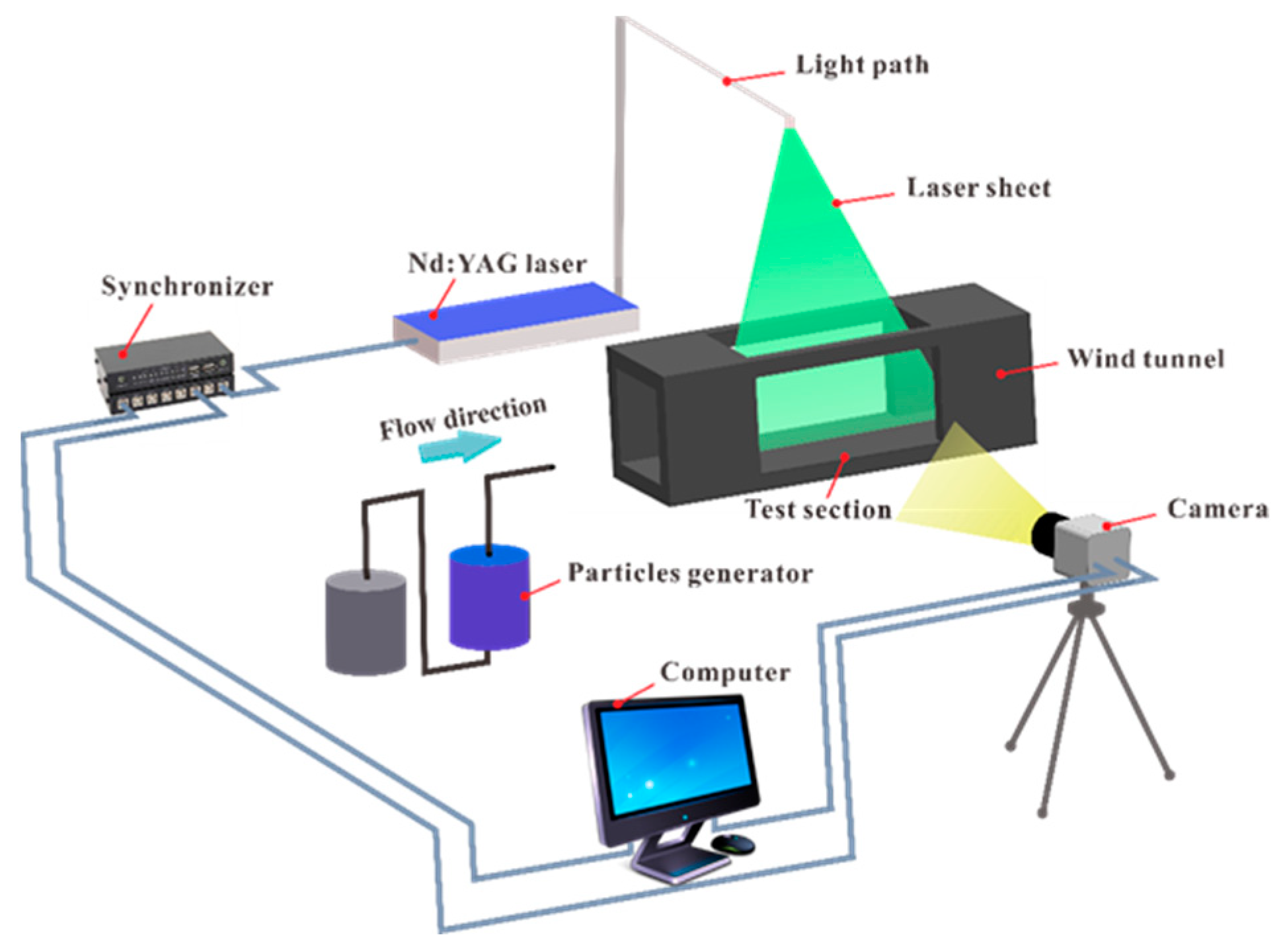
2.2. Experimental Arrangement

The experiment was conducted in the free jet supersonic wind tunnel at Nanjing University of Aeronautics and Astronautics, as shown in Figure 4, with a nozzle outlet section size of 200 mm × 200 mm.

The velocity profile of the boundary layer was acquired by measuring Pitot pressure at various distances from the wall and the local static pressure on the wall where set as at x = −20 mm on the centerline, as illustrated in Figure 5. According to the criterion that the flow velocity at the boundary layer is 0.99u₀, it can be seen that the boundary layer thickness is δ₀ = 10.24 mm. The Reynolds number Re_δ0 = 9.20 × 10⁴ is calculated using the boundary layer thickness as the characteristic scale. In contrast, higher Reynolds number (Settles et al., 1979 [12], Re_δ0 = 1.68 × 10⁶) and lower Reynolds number (Ringuette et al., 2009 [41], Re_δ0 = 3.75 × 10⁴) boundary layer velocity profiles obtained in CR-SWBLI studies under different flow conditions are presented. The incoming flow velocity profile in this study appears less fully developed compared to the Settles [12] experiment with a high Reynolds number. However, the difference is relatively small when compared to the Ringuette [41] experiment with a low Reynolds number. The boundary layer velocity profile exhibits fully developed characteristics and aligns well with the 1/7 power law curve. This indicates that the main characteristics of the incoming flow boundary layer are similar, regardless of the differences in Reynolds numbers, and the aerodynamic features of interest in the study should also be similar. Many existing studies on GV mechanisms rely on wind tunnel experiments conducted under conditions with comparable Mach numbers. Consequently, this paper aims to investigate and delineate the aerodynamic characteristics of GV structures. Furthermore, a Van Driest transformation is also performed on the raw profile, confirming its turbulent nature. The transformed u⁺ is defined as follows:

$$u_{vd}^{*}={\displaystyle \frac{1}{\kappa }}\ln z^{*}+B$$

where κ = 0.38, B = 5.1 (determined by the method proposed in Ref. [42]). The mainstream Mach number M₀ is 2.85, the mainstream velocity u₀ is 615.29 m/s, and other pertinent parameters are presented in

Table 2. Freestream flow conditions for the test.

Parameters	Value
Nominal Mach number	3.0
Actual Mach number	2.85 ± 0.01
Total temperature, K	298.2
Total pressure, kPa	100.91
Usable run time, s	>15

. Two primary factors contribute to the 5% discrepancy between the actual Mach number and the nominal Mach number. Firstly, significant viscous losses occur within the nozzle interior, which decreases the Mach number. Secondly, the IC-PLS system utilized in this study performs optimally in a high-temperature, high-humidity environment, which causes the water vapor to condense into small ice clusters, a condensation effect that also lowers the Mach number. Additionally, the displacement loss thickness δ^*, the momentum loss thickness θ, and the shape factor H can be calculated by the following formula:

$$\begin{gathered} {\delta }^{*}={\displaystyle {\int }_0^{\infty }(1-\frac{\rho u}{{\rho }_0{u}_0})}dz \\ \theta ={\displaystyle {\int }_0^{\infty }\frac{\rho u}{{\rho }_0{u}_0}(1-\frac{u}{u_0})}dz \\ H={\displaystyle \frac{\theta }{{\delta }^{*}}} \end{gathered}$$

where z is the coordinate perpendicular to the wall. Assuming that the total temperature T^* remains constant along the normal direction of the boundary layer, the density ρ within the boundary layer can be determined using the following two equations, provided that the distribution of the Mach number M in the normal direction is known:

$$\begin{gathered} T={\displaystyle \frac{T^{*}}{1+\frac{\gamma -1}{2}{M}^2}} \\ \rho ={\displaystyle \frac{p_0}{RT}} \end{gathered}$$

where γ is the specific heat ratio of air with a value of 1.4, and R is the ideal gas constant. After calculation, δ* is 1.40 mm, θ is 1.07 mm, and the shape factor H is 1.31.

The schematic diagram of the IC-PLS test system employed in this study is presented in Figure 6. This test technology, based on the Rayleigh scattering principle, enables the capturing of detailed structures within a specific two-dimensional slice of the flow field. The system primarily comprises the following components: a particle generator, a dual-channel pulsed Nd: YAG laser, a synchronization controller, a camera (Canon 1Dx Mark II, sourced from Tokyo, Japan) at a 1/15 s shutter time and 5472 × 3648 resolution, and a computer. In this study, the “particle generator” employed is not the conventional particle generator used in traditional PLS systems (such as TiO₂). Instead, it utilizes the existing water vapor in the experimental environment. As the airflow in the wind tunnel reaches supersonic speeds, the static temperature of the airflow drops significantly, causing the water vapor to rapidly condense into nanoscale ice clusters. These small ice clusters exhibit excellent flow adherence and spatial resolution within the supersonic turbulent boundary layer [31,32].

Considering the well-documented characteristics of GV reverse rotation and its large-scale distribution in the streamwise direction, along with the specific features of curved sweep compression ramp and variable swept angle, centrifugal force, and bilateral coupling interference investigated in this study, it is evident that the GV structure within the CSCR-SWBLI exhibits pronounced three-dimensional characteristics. Consequently, it becomes imperative to employ a comprehensive experimental approach and capture the GV flow field slice structure from various orientations and positions, thereby ensuring the most accurate and comprehensive depiction of the flow field.

The experiment involves three observation planes: the Y–Z plane (Laser sheet X), the X–Z plane (Laser sheet Y), and the X–Y plane (Laser sheet Z), as depicted in Figure 7 and Figure 8. Three cameras, namely, Cameras 1, 2, and 3, capture images from each plane. L_X, L_Y, and L_Z denote the specific positions of these observation surfaces. It should be noted that the position of Camera 1, as shown in Figure 7, does not impact the flow state of the model in the downstream experimental chamber. This is because the camera is positioned at the entrance of the wind tunnel, which passes through the rectification section and the nozzle downstream. For the single-sided model, the L_X values are −5 mm, 30 mm, 45 mm, and 65 mm, with the compression ramp starting at 0. The L_X = −5 mm position is upstream of the compression ramp. L_Y values include −20 mm, 0, 20 mm, 25 mm, 30 mm, and 40 mm. L_Y = −20 mm represents the undisturbed straight section unaffected by the spanwise pressure gradient. The L_Z value is 5 mm, corresponding to the middle layer of the turbulent boundary layer. Overall, these observation positions enable comprehensive capture of the characteristic structure of the GV flow field in CSCR-SWBLI. As for the double-sided model, due to its bilateral side walls, it is not feasible to set an optical observation window on the side. Consequently, the Y–Z plane is arranged as shown in Figure 9, with L_X values of −5 mm, 30 mm, 45 mm, and 65 mm.

3. Results and Discussion

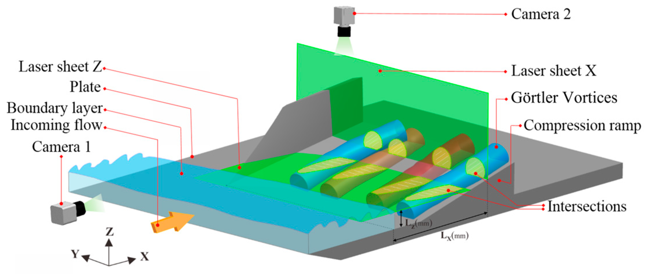
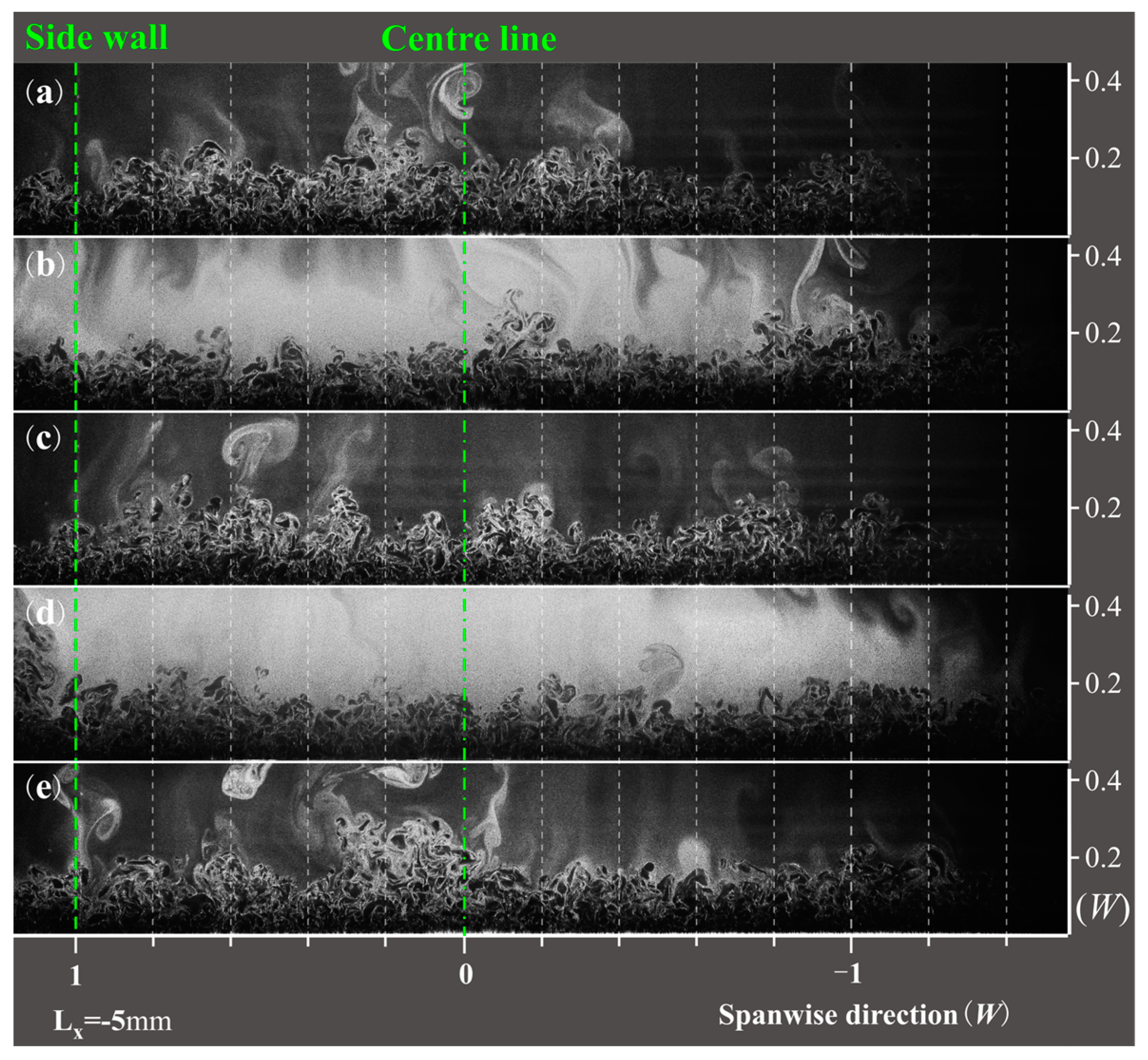
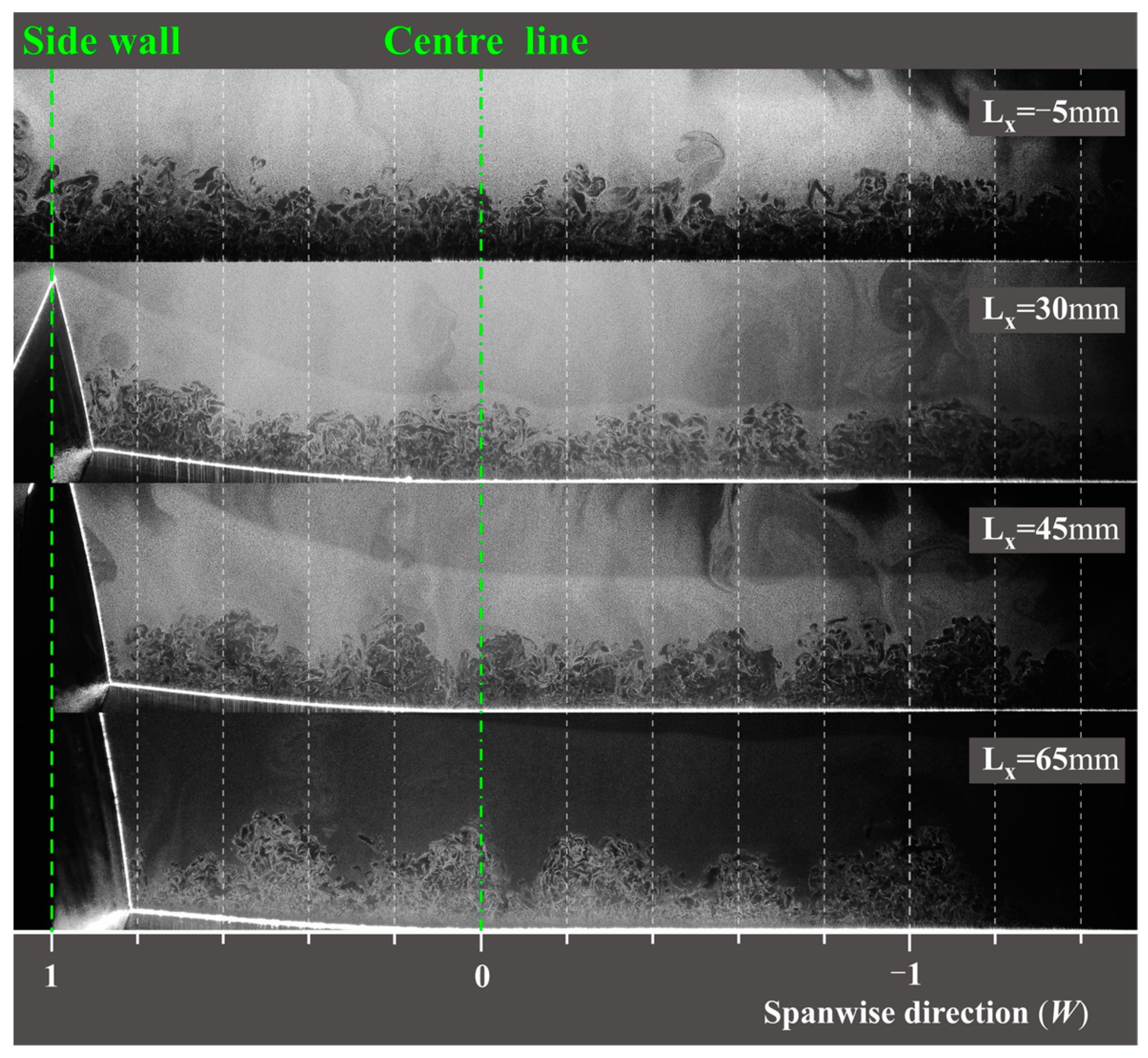
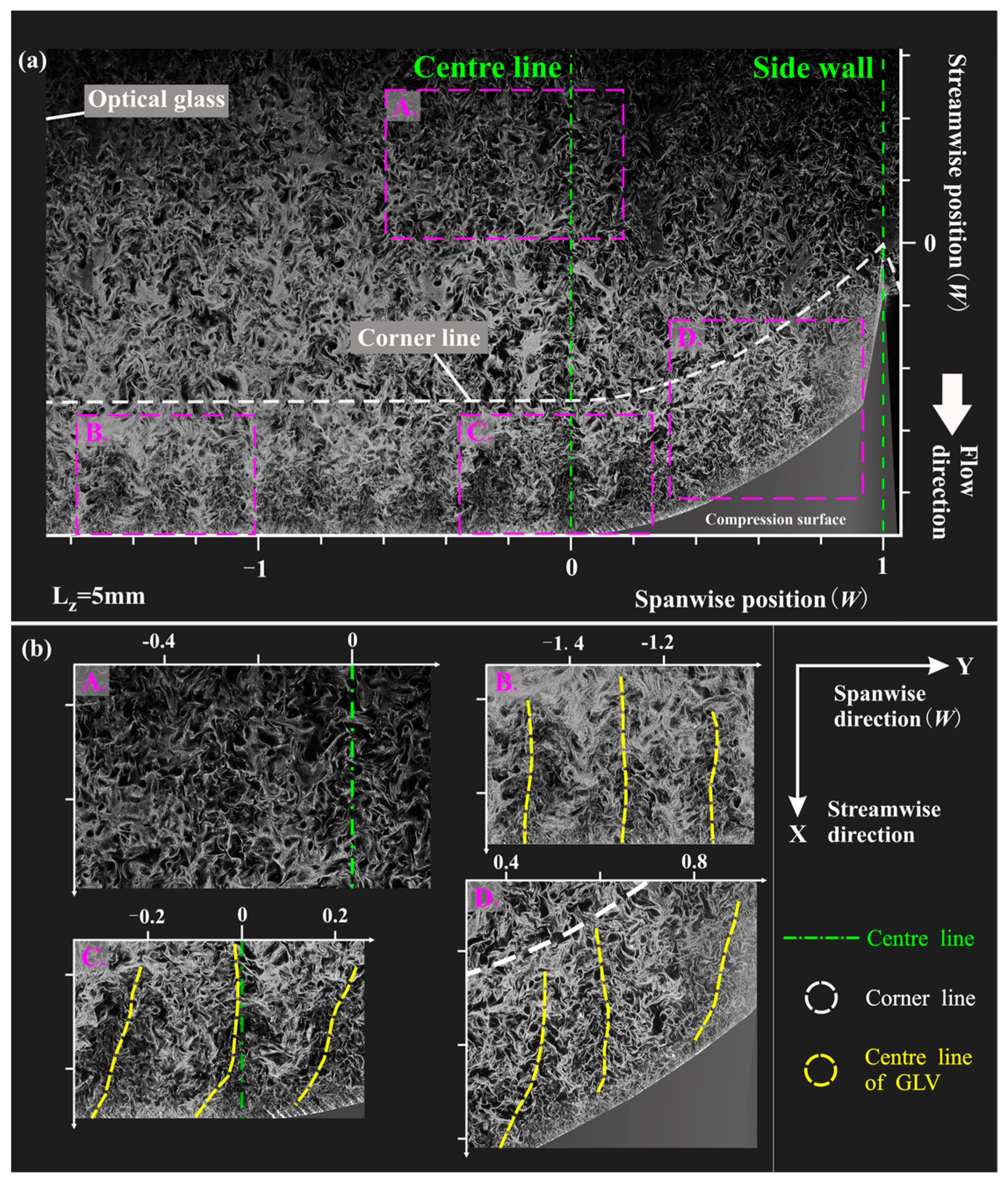
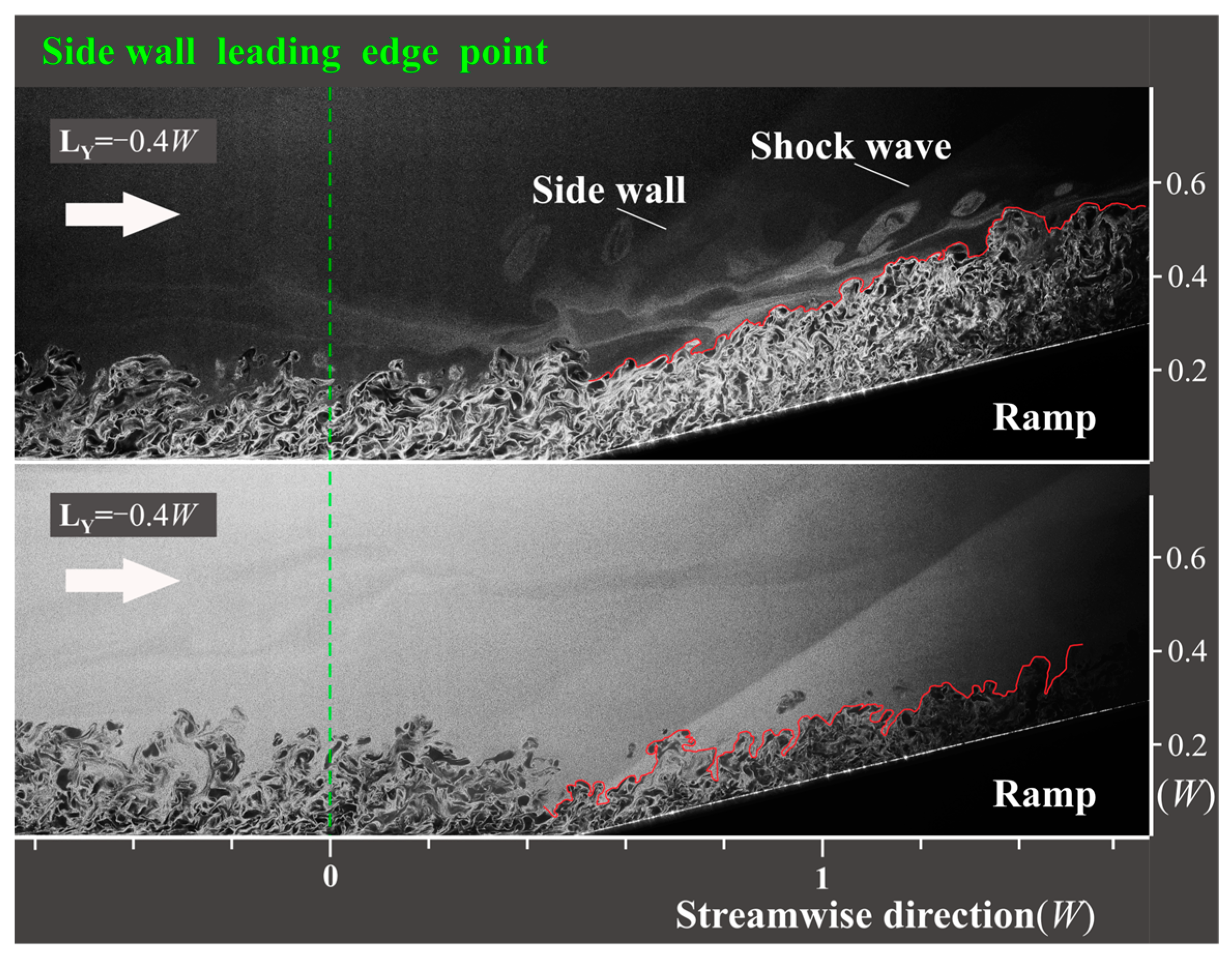
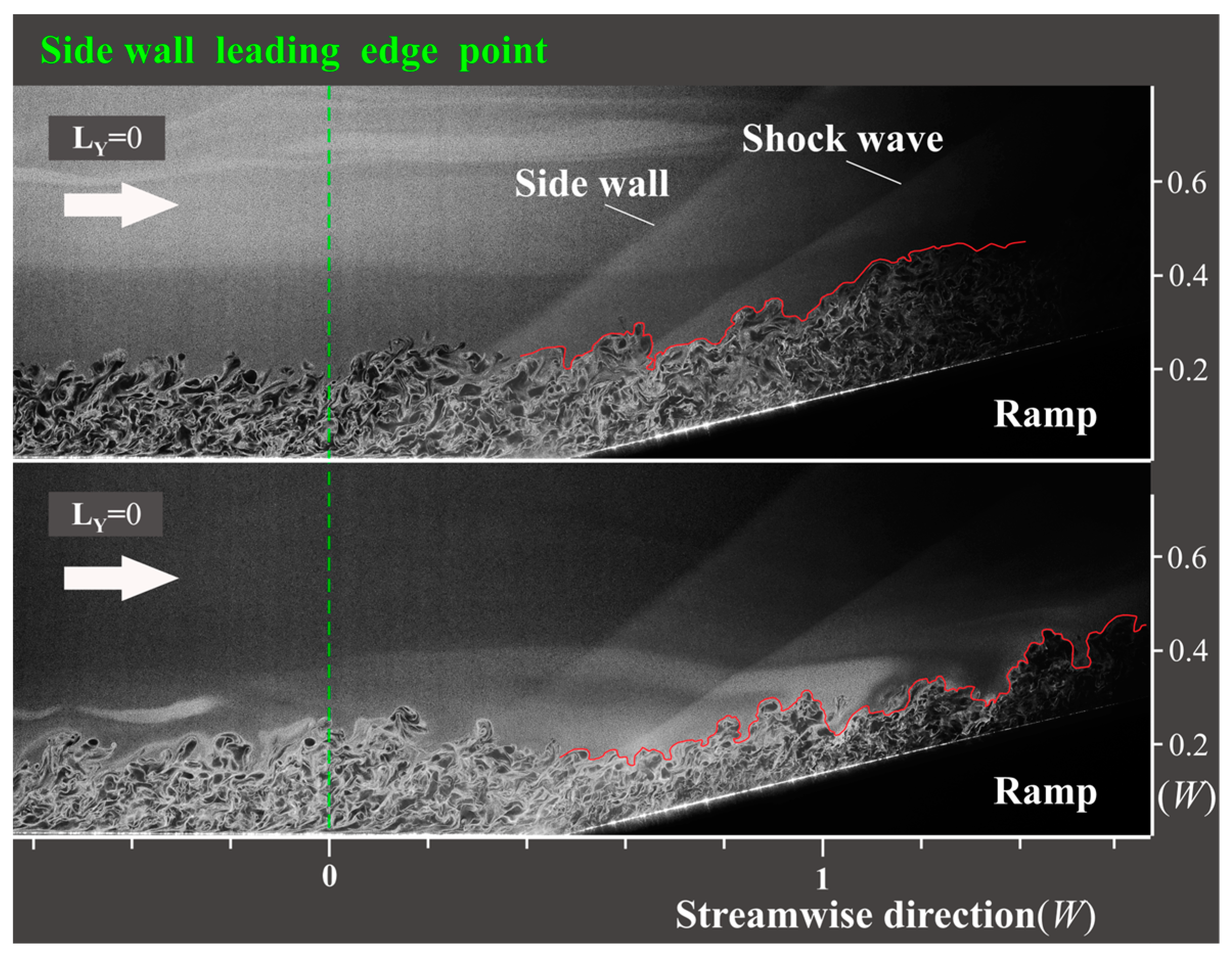
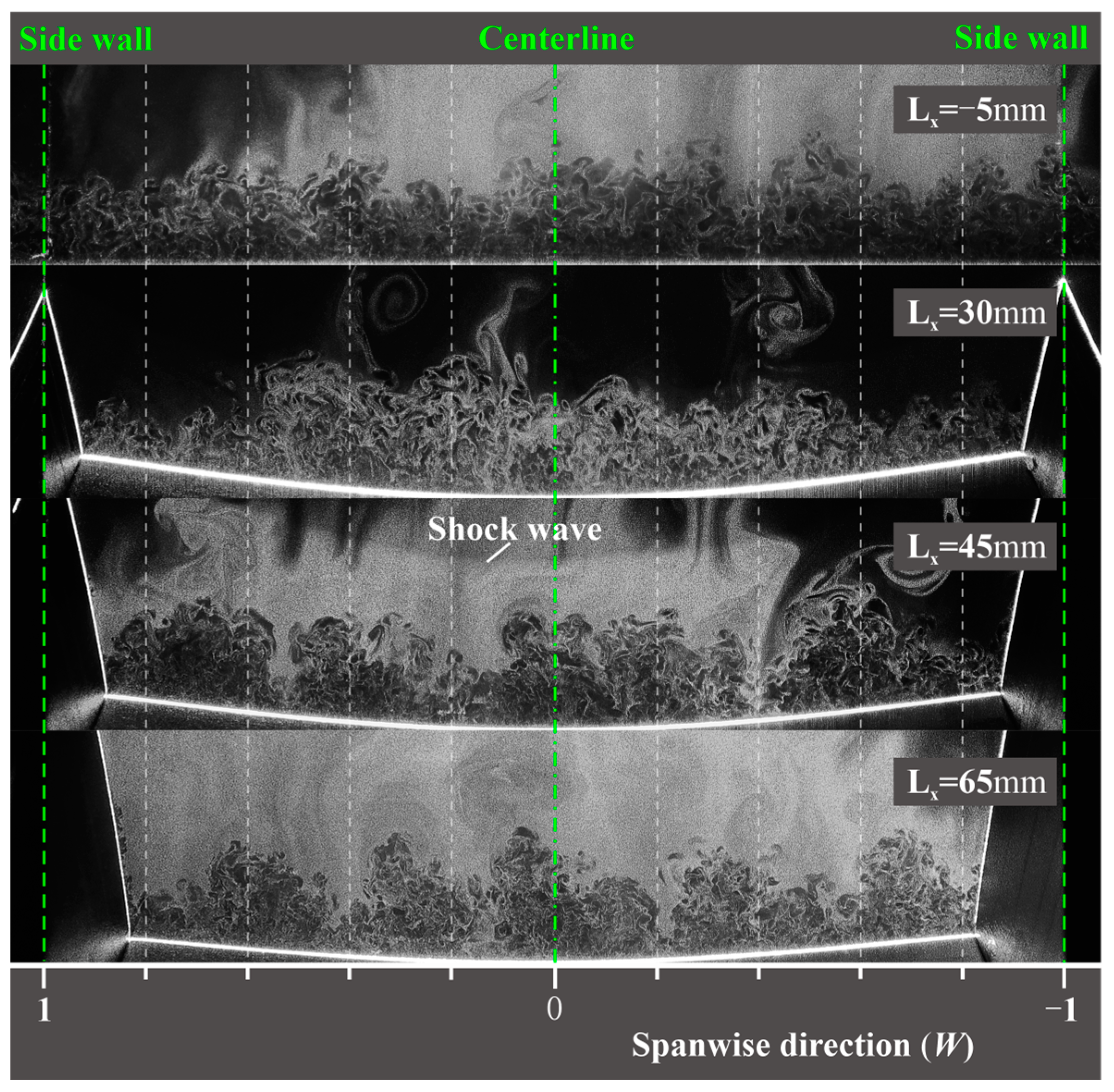
3.1. GV Structures Induced by CSCR-SWTBLI in Single-Sided Model

Figure 10 displays the IC-PLS slice image with the Y–Z plane at L_X = −5 mm. The time interval between images (a) and (e) is independent, capturing the undisturbed incoming boundary layer state upstream of the compression ramp. It should be noted that the brightness and uniformity of the image primarily depend on the plane laser. However, the plane laser cannot ensure that the entire flow field maintains high light intensity and uniformity. As a result, the brightness on the far right side of the image is low. Additionally, due to the noncontinuous uniform intensity of the plane laser, which has a response frequency of 20 Hz, it is not possible to ensure that every frame captured by the camera maintains consistent brightness and uniformity. Nevertheless, this does not affect the main observation area, so it can be disregarded. Additionally, some horizontal stripe structures in the image are caused by the burning of the model’s paint when exposed to a high-energy plane laser. Due to the multiple flow directions during sampling, a multilevel fringe structure is visually formed. The image reveals a relatively uniform boundary layer overall, with a cross-sectional scale of approximately 10 mm in the normal direction, consistent with the findings in Figure 5. Close to the wall, the incoming boundary layer is characterized by high-density and small-scale vortices, while larger-scale vortices dominate the middle and upper layers, exhibiting intermittent distribution. Notably, no well-organized large-scale vortex is observed, indicating the sufficient homogeneity of the incoming boundary layer that will not influence the downstream disturbance region, specifically the GV structures investigated in this study.

Figure 11 presents IC-PLS images with Y–Z planes positioned at L_X = −5 mm, 30 mm, 45 mm, and 65 mm, respectively, providing a comprehensive depiction of the flow field in the upstream, middle, and downstream regions of the interaction zone. These images visually demonstrate and facilitate a comparison of the generation and development of GV structures in the single-sided model. Notably, as the downstream progresses, several flow field characteristics emerge: a significant thickening of the boundary layer, mild shock wave formation, changing influence of the flow field in the curved section, increased intrusion of GVs into the boundary layer, notable variations in GV shape, and a decrease in GV quantity. Particularly in the downstream portion of the model, GV structures exhibit larger sizes but lower quantities, and there are only two GVs in the curved sections at L_X = 65 mm. This can be attributed to the thickening of the boundary layer caused by the coupling between adjacent antirotating vortices and their rotational motion, resulting in increased entrainment of internal fluid within the boundary layer. Consequently, this process greatly enhances the mixing effect between the mainstream and low-energy flow within the boundary layer. The introduction of this paper highlights the research significance of GVs as a noninvasive mixing technology. Given the inherent nonsteadiness of GVs, this mixing effect is expected to positively impact downstream combustion chambers. Additionally, the influence of the spanwise pressure gradient in the curved section varies with the development of the flow field. Specifically, this influence is more pronounced in the front section of the model (L_X = 30, 45 mm). This is characterized by the coupling of adjacent antirotating vortices and the displacement of the boundary layer towards the central plane. However, the influence gradually diminishes in the rear section (L_X = 45, 65 mm).

Figure 12 illustrates the IC-PLS image with the X–Y plane at L_Z = 5 mm, presenting a slice of the flow field within the middle layer of the boundary layer. The flow direction is depicted from top to bottom, with the white dashed line representing the leading-edge line of the compression ramp, and the yellow dashed line indicating the central axis of the GV. As this section is positioned above the separation bubble’s thickness, the image does not reflect the characteristics of the separation bubble. In Figure 12b, magnified images of four distinct regions (A, B, C, and D) identified in Figure 12a are showcased. The undisturbed incoming flow is observed upstream of the white dashed line, while the downstream region exhibits the boundary layer traversing the separated shock wave on the compression ramp, characterized by black striped GV structures. The spanwise scale of the GVs generally corresponds to the local boundary layer’s thickness, aligning with the findings from the Y–Z plane analysis. In the straight section, the GV structures predominantly align with the flow direction, whereas in the curved section, the GV structures exhibit varying degrees of curvature due to the influence of the spanwise pressure gradient. However, GVs are highly susceptible to upstream flow due to its significant instability. The absence of any vortex disturbance in the incoming boundary layer cannot be guaranteed. Consequently, when large-scale vortex structures are present upstream, they inevitably interact with GVs in the interaction region to form more intense strip vortex structures (such as those located along the centerline). Nevertheless, this phenomenon is rarely observed in the flow field. Notably, adjacent antirotating vortices demonstrate close connections and coupling. In Figure 12b, region A depicts the undisturbed incoming boundary layer upstream of the compression plane. The inner boundary layer exhibits dense and small vortex structures, devoid of any prominent large-scale vortex groups or streamwise vortex structures. This observation confirms the uniformity and absence of additional downstream interference in the incoming flow. The B region illustrates the GV structure in the straight section, revealing a near coaxial alignment with the flow direction. Region C corresponds to the flow field near the central plane, where the curved section displaces the local boundary layer along the development direction, resulting in an evident curvature of the central axis of the GVs in this region. Region D captures the flow field within the curved section, displaying a pronounced curvature of the central axis of the GV, which varies in relation to the local swept angle. Due to the transverse pressure gradient in the curved section, the GVs in the C and D regions will experience varying degrees of deflection. As the flow progresses downstream, these deflected GVs will inevitably interact and merge with adjacent GVs, leading to a gradual reduction in their quantity along the downstream direction. Adjacent flow vortices exhibit strong coupling, and the gap between them is filled with tighter and smaller vortices compared to the corresponding straight section. To illustrate the behavior of GVs at the same position over different times, ten frames of IC-PLS images were collected. Due to space constraints, it is impractical to display all ten frames in this paper. Therefore, the frames were averaged, and the results are presented in Figure 13. It can be seen that due to the strong nonsteadiness of GVs, their spanwise position is not fixed, leading to no obvious strip vortex structure found in the results after averaging.

Figure 14 and Figure 15 present X–Z plane images of IC-PLS at L_Y = −0.4W and 0, respectively. L_Y = −0.4W corresponds to the straight section unaffected by the spanwise pressure gradient of the curved section, while L_Y = 0 represents the center plane influenced by the spanwise pressure gradient. Both figures capture the same position but at different times. The ramp-induced oblique shock wave is clearly visible, and the sudden brightness in the flow field, attributed to the density increase after the shock, is readily apparent. Although the instantaneous image does not provide insight into the time-averaged state of the boundary layer after the oblique shock, it is evident that the incoming boundary layer remains relatively unchanged over time, demonstrating uniform performance. From the various observation perspectives explored above, it is apparent that the GV displays high levels of unsteadiness. Specifically, within this section, it becomes evident that the thickness of the boundary layer following the shock wave significantly varies over time at the same position. This variation confirms the intermittent nature of the GV induced by CSCR-SWBLI and highlights the instability of the spanwise position. Moreover, the morphology of the boundary layer post-shock wave appears relatively flat in the straight section but in the center plane; however, there are some bulging profiles that make the boundary layer appear to fluctuate slightly. These findings align with the aforementioned results, suggesting that the GV structure in the central plane experiences bending effects due to the influence of the curved section.

Figure 16 showcases IC-PLS images depicting X–Z planes at various spanwise positions in the curved segment, specifically at L_Y = 0.4, 0.5, 0.6, and 0.8W. The purpose is to compare the flow field slice states at different locations within the spanwise dimension. The structure of the GVs, as illustrated in Figure 12, demonstrates that GVs bend towards the center plane to varying degrees due to transverse pressure gradients. This results in multiple curved GV cross-sections appearing in the X–Z observation plane at the same location, as depicted in Figure 16, which represents the vortex packet structure. The number of vortex packets near the center plane is significantly higher than near the sidewall, and the vortex packet structures are more stable, further confirming that the GVs bend towards the center plane. Consequently, the distinct axial characteristics of GVs in the curved section are further validated.

3.2. GV Structures Induced by CSCR-SWTBLI in Single-Sided Model at M₀ = 2.66

To investigate the GV structure in the context of CSCR-SWTBLI under varying Mach number conditions, the flow field is examined at an incoming Mach number of 2.66. This is achieved by increasing the model’s angle of attack to +4° within this section, as displayed in Figure 17. Figure 18 displays IC-PLS images in the Y–Z plane at L_X = −5 mm, 30 mm, 45 mm, and 65 mm, respectively. These images are juxtaposed with the corresponding positions at M₀ = 2.85, as discussed earlier.

The overall development of the flow field state aligns with that of the M₀ = 2.85 condition, and the presence of visible GV structures on the compression ramp is evident. However, there are several notable characteristics specific to this condition. Firstly, the shock wave induced by the front of the plate (referred to as Shock Wave 1 in the figure) is relatively straight, indicating a well-established flow field and a more uniform incoming boundary layer along the spanwise direction after adjusting the model’s angle of attack. In contrast, the compression shock wave induced by the compression ramp (referred to as Shock Wave 2 in the figure) exhibits varying degrees of fluctuation due to the influence of the vortex envelope structure. Secondly, after the boundary layer passes through the compression shock wave at the plate’s leading edge, there is a greater density reflection observed upstream in the interaction region, resulting in the almost disappearance of shedding vortices in the upper layer of the boundary layer. The presence of small-scale fluctuations resembling the vortex envelope structure along the spanwise direction in the boundary layer is noteworthy. These fluctuations are a result of the boundary layer passing through a weak CR-SWBLI. While the stability of the boundary layer in this state is not as high as that observed in the M₀ = 2.85 condition, the intensity and extensional periodicity of these small-scale fluctuations are noticeably weaker compared to the GV structure on the downstream compression ramp. Additionally, upon examining the IC-PLS slice images at L_X = 30 mm, 45 mm, and 65 mm, an increase in the density of GVs on the compression plane is observed. However, considering the nonconstancy of GVs, their periodicity and intensity do not differ significantly from the M₀ = 2.85 state.

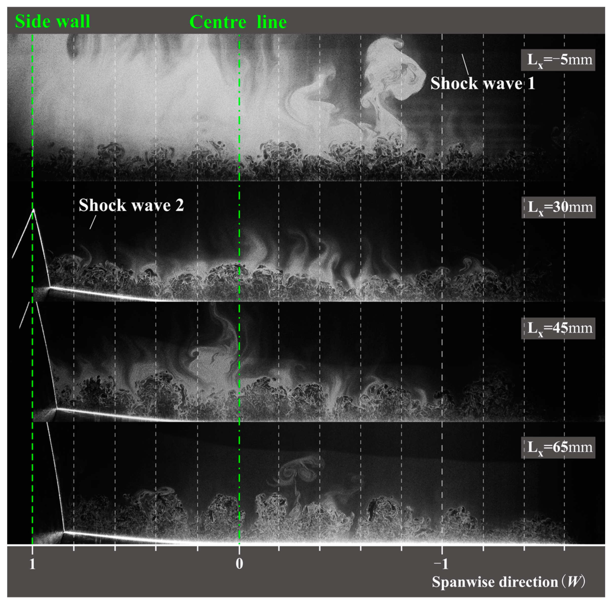
3.3. GV Structures Induced by CSCR-SWTBLI in Double-Sided Model

Figure 19 presents the IC-PLS images in the Y–Z planes of the double-sided model at varying positions: L_X = −5 mm, 30 mm, 45 mm, and 65 mm. These images provide insight into the vortex states within the upper, middle, and lower sections of the interaction region. Observations reveal that the boundary layer upstream of the interaction region demonstrates good uniformity, suggesting consistency with the flow state exhibited in the single-sided model. At L_X = 30 mm, the boundary layer on both sides of the corner region appears thinner, and due to the spanwise pressure gradient, the boundary layer accumulates on the symmetry plane, resulting in mutual coupling of the vortex structure. As L_X = 45 mm is reached, the overall scale of each vortex increases, with relatively independent behavior and reduced coupling degree. When L_X = 65 mm is considered, the vortex morphology exhibits greater stability, with vortices displaying increased independence. Notably, there is minimal coupling observed in the middle and upper layers of the boundary layer, and the number of vortices remains relatively stable at 5, slightly more than the number of curved segments of the single-sided model at the same position. In comparison to the single-sided model, several similarities and differences are apparent. Firstly, the boundary layer thickness notably increases, while the shock surface gradually flattens. Additionally, the influence vortex shape varies at different degrees in the curved section. The extent of GV intrusion into the boundary layer intensifies, while the downstream development of GVs maintains stability and decreases in number. Furthermore, the cross-section of the vortex consistently aligns with the local boundary layer thickness. However, an important distinction arises due to the coupling of the two sidewalls, resulting in the presence of a persistent large-scale vortex in the symmetry plane, and the overall structure of the flow field is symmetric, so the number of GVs on the compression plane is always odd. It is important to note that the time-independent IC-PLS technique was employed to examine the aerodynamic characteristics of the GV structure in CSCR-SWBLI under typical design parameters of the test model. Consequently, due to the limitations of the test conditions, a detailed quantitative analysis of the GV structure will be conducted in future research.

3.4. Verification of the Existence of GV Structures Induced by CSCR-SWBLI

The time-averaged flow field of CSCR-SWBLI was examined through both oil flow experiments and numerical simulations in Ref [40]. Figure 20 and Figure 21 depict the flow topologies for the single-sided and double-sided models of CSCR-SWBLI, respectively. It should be explained that these calculated results were verified to be accurate enough in calculating the size of the separation region by comparing them with the oil flow results. In the single-sided model, flow separation occurs after passing through the shock wave, with the maximum separation observed at point A in Figure 20. Notably, the separation region exhibits a distinct “scimitar” shape, deviating from conventional CR-SWBLI and SCR-SWBLI patterns. Conversely, in the overall flow topology of the double-sided CSCR-SWBLI relative to the central plane, the separation bubble is larger compared to the single-sided model. The separation line forms a node, N1, on the symmetry plane, while the reattachment line forms a saddle point, S1, on the symmetry plane. Moreover, the separation region originates from the corner regions on both sides and converges towards the plane of symmetry, where oil accumulation is observed. As a result, the separation scale reaches its maximum on the central plane, leading to the formation of a distinctive “crescent” shape in the separation region. It is noteworthy that both experimental and numerical findings consistently demonstrate a uniform wall flow structure. Notably, no stable streamwise vortex structure is observed, providing further evidence of the inherent instability and unsteadiness associated with the streamwise strip vortex structure in SWBLI.

This section aims to validate the presence of GV structures in CSCR-SWBLI, as captured by the aforementioned IC-PLS experiment, utilizing established determination methods outlined in the literature. The flow profile structure exhibits similarities to CR-SWBLI, as the curved swept compression ramp model employed in this study can be considered analogous to a variable swept angle back-swept compression ramp model. Figure 22 illustrates the time-averaged perspective, wherein the boundary layer separates upon encountering the compression ramp. This separation gives rise to two distinct flow regions: the main stream portion and the reflux-induced separation region (indicated by the blue arrow), separated by the shear layer originating from the separation point (indicated by the red dashed line).

GVs are the centrifugal instability of the turbulence boundary layer, which must be closely related to the degree of deflection of the fluid in the flow field. The Görtler number (G_T) [43] and the Floryan (F) experiential criterion [44] have been applied to multiple investigations on supersonic flows to assess the existence of GVs [31,32,45,46,47]. Smits [48] proposed a determination method for compressible turbulence flow based on Görtler number (G_T), and its definition formula is as follows:

$$G_T={\displaystyle \frac{\theta }{0.018{\delta }^{*}}}\sqrt{{\displaystyle \frac{\theta }{\left|r\right|}}}$$

where θ represents the momentum loss thickness of the incoming boundary layer, δ^* represents the displacement loss thickness, r represents the actual deflection radius of the flow, and G_T > 0.6 is taken as the criterion for the existence of GVs. In addition, the Floryan number (F) was defined as follows:

$$F={\displaystyle \frac{{\delta }_0}{r}}$$

where δ₀ represents the thickness of the incoming boundary layer, r represents the actual deflection radius of the flow, and it is determined that the GV appears in the flow when F > 0.01.

In general, when determining the boundary layer parameters (δ*, θ, δ₀) under specific incoming flow conditions, the existence of GVs is solely dependent on the actual deflection radius value, denoted as r. Analysis of the two judgment formulas reveals that both the G_T number and F number decrease as the actual deflection radius, r, increases. This implies that when r exceeds its actual value, the resulting G_T number or F value will be underestimated, leading to a more conservative assessment. Consequently, such an approach ensures a more realistic and reliable judgment outcome.

When examining the simplified time-averaged flow profile depicted in Figure 22, it becomes evident that the flow experiences two distinct deflections at the separation and reattachment points. However, accurately determining the specific positions of the shear layer corresponding to the separation deflection radius and reattached deflection radius proves challenging during actual calculations, leading to inevitable errors in the obtained values. To address this, Navarro [49] proposed a simplified model for assessing the existence of GVs in CR-SWBLI. They considered the flow as undergoing a single deflection at the compression corner, thereby resulting in a single deflection radius. Building upon this concept, Zhuang [47] further simplified the CR-SWBLI model. After identifying the reattachment position, they constructed an arc tangent to the horizontal plane through the reattachment point. The starting point of the flow deflection was then determined as the tangent point between the arc and the horizontal plane, with the resulting curvature radius serving as the deflection radius. Consequently, the obtained deflection radius is significantly larger than the actual separation and reattachment deflection radii, leading to a more conservative estimation of the G_T number or F value.

Based on the oil flow results depicted in Figure 20 and Figure 21, it is evident that the CSCR-SWBLI separation point of both the single-sided and double-sided models can be represented by a curve tangent to the local compression surface at the separation point. This curve allows the determination of a deflection radius, which is found to exceed the actual separation and reattachment deflection radii. Consequently, the obtained judgment results are deemed conservative and reliable. Subsequently, the G_T number and F number for CSCR-SWBLI in this study are calculated using the aforementioned formulas. The resulting variation curves along the spanwise direction are presented in Figure 23 and Figure 24, respectively. Notably, regardless of the determination method employed (based on G_T number or F number), the calculated values consistently surpass the critical value. Hence, it can be concluded that the investigated CSCR-SWBLI flow field does, indeed, exhibit GV structures.

4. Conclusions

This paper investigated the GV structures in the CSCR-SWBLI phenomenon caused by the compression ramp of the inward-turning inlet’s front edge under integrated design conditions. This study employed IC-PLS technology, utilizing multiple observation orientations and positions. The existence of GVs in CSCR-SWBLI was verified through the GT number and F-number criteria. The key findings are as follows:

• The quantity and spanwise position of GVs exhibit strong intermittency and are not fixed. The cross-section scale is consistently equivalent to the boundary layer thickness.
• Comparing the flow field at a +4° angle of attack reveals minimal changes in overall flow field characteristics, except for an increase in boundary layer density.
• The double-sided model demonstrates a stable, downstream-developing, large-scale vortex in the symmetry plane as a result of coupling effects. Notably, GV structures always appear in odd numbers. More importantly, the mixing effect of GVs on the boundary layer and the main stream within the inlet was found to improve the uniformity of the internal flow field and reduce distortion, and this provides a new research idea for the inlet designers to study the development and control of the boundary layer of the inward turning inlet.
• Calculation of the GT number and F number for both single-sided and double-sided CSCR-SWBLI enables the determination of spanwise variation patterns. Both values significantly exceed the critical threshold, providing further evidence for the existence of GVs in CSCR-SWBLI.

References

- Smart, M.K. How much compression should a scramjet inlet do? AIAA J. 2012, 50, 610–619. [Google Scholar] [CrossRef]
- Mölder, S.; Szpiro, E.J. Busemann inlet for hypersonic speeds. J. Spacecr. Rocket. 1966, 3, 1303–1304. [Google Scholar] [CrossRef]
- You, Y.C.; Liang, D.W.; Huang, G.P. Cross section controllable hypersonic inlet design using streamline-tracing and osculating axisymmetric concepts. In Proceedings of the 43rd AIAA/ASME/SAE/ASEE Joint Propulsion Conference & Exhibit, Cincinnati, OH, USA, 8–11 July 2007. [Google Scholar]
- Billig, F.S.; Kothari, A.P. Streamline tracing: Technique for designing hypersonic vehicles. J. Propuls. Power 2000, 16, 465–471. [Google Scholar] [CrossRef]
- Rowan, J.G.; Michael, K.S. Design of modular shape-transition inlets for a conical hypersonic vehicle. J. Propuls. Power 2013, 29, 832–838. [Google Scholar]
- Samuel, E.O.; Charles, J.T.; John, W.S. Inward-turning streamline-traced inlet design method low-boom low-drag applications. J. Power Propuls. 2016, 32, 1178–1189. [Google Scholar]
- Li, Y.; Zheng, X.; Shi, C.; You, Y. Integration of inward-turning inlet with airframe based on dual-wave rider concept. Aerosp. Sci. Technol. 2020, 107, 106266. [Google Scholar] [CrossRef]
- Malo, F.J.; Gaitonde, D.V.; Ruffin, S. Analysis of an innovative inward turning inlet using an Air-JP8 combustion mixture at Mach 7. In Proceedings of the 36th AIAA Fluid Dynamics Conference and Exhibit, San Francisco, CA, USA, 5–8 June 2006. [Google Scholar]
- Babinsky, H.; Harvey, J.K. Shock Wave-Boundary-Layer Interactions; Cambridge University Press: Cambridge, UK, 2011; p. 32. [Google Scholar]
- Delery, J.; Marvin, G.J. Shock Wave–Boundary Layer Interactions; AGARD: Neuilly, France, 1986. [Google Scholar]
- Settles, G.S.; Vas, I.E.; Bogdonoff, S.M. Details of a shock-separated turbulent boundary layer at a compression corner. AIAA J. 1976, 14, 1709–1715. [Google Scholar] [CrossRef]
- Settles, G.S.; Fitzpatrick, T.J.; Bogdonoff, S.M. Detailed study of attached and separated compression corner flowfields in high Reynolds number supersonic flow. AIAA J. 1979, 17, 579–585. [Google Scholar] [CrossRef]
- Smits, A.J.; Muck, K.C. Experimental study of three shock wave/turbulent boundary layer interactions. J. Fluid Mech. 1987, 182, 291–314. [Google Scholar] [CrossRef]
- Elfstrom, G.M. Turbulent hypersonic flow at a wedge-compression corner. J. Fluid Mech. 1972, 53, 113–127. [Google Scholar] [CrossRef]
- Dolling, D.S.; Or, C.T. Unsteadiness of the shock wave structure in attached and separated compression ramp flows. Exp. Fluids 1985, 3, 24–32. [Google Scholar] [CrossRef]
- Loginov, M.S.; Adams, N.A.; Zheltovodov, A.A. Large-eddy simulation of shock-wave/turbulent-boundary-layer interaction. J. Fluid Mech. 2006, 565, 135–169. [Google Scholar] [CrossRef]
- Grilli, M.; Hickel, S.; Adams, N.A. Large eddy simulation of a supersonic turbulent boundary layer over a compression–expansion ramp. Int. J. Heat Fluid Flow 2013, 42, 79–93. [Google Scholar] [CrossRef]
- Zheltovodov, A.A. Some advances in research of shock wave-turbulent boundary. In Proceedings of the 44th AIAA Aerospace Sciences Meeting and Exhibit, Reno, NV, USA, 9–12 January 2006. [Google Scholar]
- Zheltovodov, A.A. Advances and problems in modeling of shock wave turbulent boundary layer interactions. In Proceedings of the International Conference on the Methods of Aero Physical Research, Novosibirsk, Russia, 1–5 July 2024. [Google Scholar]
- Zheltovodov, A.A.; Maksimov, A.; Shilein, E. Development of turbulent separated flows in the vicinity of swept shock waves. In The Interactions of Complex; Springer: Berlin/Heidelberg, Germany, 1987; pp. 67–91. [Google Scholar]
- Settles, G.S.; Teng, H. Cylindrical and conical flow regimes of three-dimensional shock/boundary layer interactions. AIAA J. 1984, 22, 194–200. [Google Scholar] [CrossRef]
- Settles, G.S.; Perkins, J.J.; Bogdonoff, S.M. Investigation of three-dimensional shock/boundary layer interaction at swept compression corners. AIAA J. 1980, 18, 779–785. [Google Scholar] [CrossRef]
- Knight, D.D.; Horstman, C.; Bogdonoff, S.M. Structure of supersonic turbulent flow past a swept compression corner. AIAA J. 1992, 30, 890–896. [Google Scholar] [CrossRef]
- Görtler, H. Instabilität laminarer Grenzschichten an konkaven Wänden gegenüber gewissen dreidimensionalen Störungen. ZAMM-J. Appl. Math. Mech./Z. Angew. Math. Mech. 1941, 21, 250–252. [Google Scholar] [CrossRef]
- Tong, F.; Li, X.; Duan, Y.; Yu, C. Direct numerical simulation of supersonic turbulent boundary layer subjected to a curved compression ramp. Phys. Fluids 2017, 29, 125101. [Google Scholar] [CrossRef]
- Wang, Q.; Wang, Z.; Zhao, Y. An experimental investigation of the supersonic turbulent boundary layer subjected to concave curvature. Phys. Fluids 2016, 28, 96–104. [Google Scholar] [CrossRef]
- Chen, X.; Zhu, Y.; Lee, C. Interactions between second mode and low-frequency waves in a hypersonic boundary layer. J. Fluid Mech. 2017, 820, 693–735. [Google Scholar] [CrossRef]
- Loginov, M.S. Large-Eddy Simulation of Shock Wave/Turbulent Boundary Layer Interaction; Technische Universität München: Munich, Germany, 2006. [Google Scholar]
- Tokura, Y.; Maekwa, H. Direct numerical simulation of impinging shock wave/transitional boundary layer interaction with separation flow. J. Fluid Sci. Technol. 2011, 6, 765–779. [Google Scholar] [CrossRef]
- Pasquariello, V.; Hickel, S.; Adams, N.A. Unsteady effects of strong shock-wave/boundary-layer interaction at high Reynolds number. J. Fluid Mech. 2017, 823, 617–657. [Google Scholar] [CrossRef]
- Zhuang, Y.; Tan, H.J.; Li, X.; Sheng, F.J.; Zhang, Y.C. Görtler-like vortices in an impinging shock wave/turbulent boundary layer interaction flow. Phys. Fluids 2018, 30, 061702. [Google Scholar] [CrossRef]
- Li, X.; Zhang, Y.; Yu, H.; Lin, Z.K.; Tan, H.J.; Sun, S. Görtler vortices behavior and prediction in dual-incident shock-wave/turbulent-boundary-layer interactions. Phys. Fluids 2022, 34, 106103. [Google Scholar] [CrossRef]
- Ciolkosz, L.; Spina, E. An experimental study of Görtler vortices in compressible flow. In Proceedings of the 42nd AIAA/ASME/SAE/ASEE Joint Propulsion Conference & Exhibit, Sacramento, CA, USA, 9–12 July 2006; p. 4512. [Google Scholar]
- Swearingen, J.D.; Blackwelder, R.F. The growth and breakdown of streamwise vortices in the presence of a wall. J. Fluid Mech. 1987, 182, 255–290. [Google Scholar] [CrossRef]
- Sun, M.; Sandham, N.D.; Hu, Z. Turbulence structures and statistics of a supersonic turbulent boundary layer subjected to concave surface curvature. J. Fluid Mech. 2019, 865, 60–99. [Google Scholar] [CrossRef]
- Ren, J.; Fu, S. Nonlinear development of the multiple Görtler modes in hypersonic boundary layer flows. In Proceedings of the 43rd AIAA Fluid Dynamics Conference, San Diego, CA, USA, 24–27 June 2013; p. 2467. [Google Scholar]
- Ren, J.; Fu, S. Secondary instabilities of Görtler vortices in high-speed boundary layer flows. J. Fluid Mech. 2015, 781, 388–421. [Google Scholar] [CrossRef]
- Roghelia, A.; Olivier, H.; Egorov, I.; Chuvakhov, P. Experimental investigation of Görtler vortices in hypersonic ramp flows. Exp. Fluids 2017, 58, 1–15. [Google Scholar] [CrossRef]
- Chen, L.; Zhang, Y.; Xue, H.; Chuvakhov, P. Experimental and numerical investigation of shock wave/boundary layer interactions induced by curved back-swept compression ramp. Aerosp. Sci. Technol. 2023, 142, 108639. [Google Scholar] [CrossRef]
- Zhang, Y.; Chen, L.; Tan, H.J.; Wang, C.; Cheng, F.; Li, C. Visualization of curved swept shock wave/turbulent boundary layer interaction in supersonic flow. J. Vis. 2020, 24, 1–7. [Google Scholar] [CrossRef]
- Ringuette, M.J.; Bookey, P.; Wyckham, C.; Smits, A.J. Experimental Study of a Mach 3 Compression Ramp Interaction at Re{theta} = 2400. AIAA J. 2009, 47, 373–385. [Google Scholar] [CrossRef]
- Anthony, K.; Manoochehr, K. A Method for Estimating Wall Friction in Turbulent Wall-Bounded Flows. Exp. Fluids 2008, 55, 773–780. [Google Scholar]
- Görtler, H. On the Three-Dimensional Instability of Laminar Boundary Layers on Concave Walls; National Advisory Commitee for Aeronautics Technical Memorandum: Hampton, VA, USA, 1954; p. 1375. [Google Scholar]
- Floryan, J.M. On the Görtler instability of boundary layers. Prog. Aerosp. Sci. 1991, 28, 235–271. [Google Scholar] [CrossRef]
- Priebe, S.; Tu, J.H.; Rowley, C.W.; Martín, M.P. Low-frequency dynamics in a shock-induced separated flow. J. Fluid Mech. 2016, 807, 441–477. [Google Scholar] [CrossRef]
- Duan, J.Y.; Li, X.; Li, X.L.; Liu, H. Direct numerical simulation of a supersonic turbulent boundary layer over a compression-decompression corner. Phys. Fluids 2021, 33, 065111. [Google Scholar] [CrossRef]
- Zhuang, Y.; Tan, H.J.; Liu, Y.Z.; Zhang, Y.C.; Ling, Y. High-Resolution Visualization of Görtler-Like Vortices in Supersonic Compression Ramp Flow. J. Vis. 2017, 20, 505–508. [Google Scholar] [CrossRef]
- Smits, A.J.; Dussauge, J.P. Turbulent Shear Layers in Supersonic Flow; Springer Science & Business Media: Berlin/Heidelberg, Germany, 2006. [Google Scholar]
- Navarro-Martinez, S.; Tutty, O.R. Numerical simulation of Görtler vortices in hypersonic compression ramps. Comput. Fluids 2005, 34, 225–247. [Google Scholar] [CrossRef]