Purchasing Power Parity in Transition Countries: Panel Stationary Test with Smooth and Sharp Breaks

Abstract

This study examines whether the long-run purchasing power parity (PPP) holds in transition economies (Bulgaria, the Czech Republic, Hungary, Latvia, Lithuania, Poland, Romania and Russia) using monthly data over the 1995–2011 period. We apply a recently introduced panel stationary test, which accounts for sharp breaks and smooth shifts. The results indicate that the PPP holds only in two countries (i.e., Lithuania and Poland).

1. Introduction

Purchasing power parity (PPP) remains a cornerstone of many theoretical models in international finance. In its simplest form, PPP states that the exchange rate between two currencies should be equal to the ratio of two associated price levels. Alternatively, if we combine the nominal exchange rate and relative prices together to get the real exchange rate, this new measure should converge to its mean in the long run for the PPP to hold. Therefore, a non-stationary real exchange rate indicates that there is no long-run relationship between the nominal exchange rate, domestic prices and foreign prices, thereby invalidating the PPP.

Given the importance of the PPP hypothesis in open economy macroeconomic models and for constructing fundamental equilibrium exchange rates, the long-run PPP relationship has been empirically investigated extensively, using different approaches. The literature related to transition economies has already been reviewed by Bahmani-Oskooee and Hegerty [1] and need not be repeated here. The most common approach to test the PPP today is to apply unit root tests on real exchange rate series and to determine the mean reverting properties of them. As the review indicates, the results are mixed, and they depend on whether one uses linear or non-linear tests or time-series versus panel tests. Generally, since panel unit root tests utilize much more observations, they are said to be more powerful than time-series tests applied to data from an individual country.

Even within panel tests, failure to account for structural breaks in real exchange rates is said to contribute to the failure of PPP. A few studies led by Im et al. [2] have developed panel unit root tests with structural breaks, allowing for the break dates to be different across countries of the panel. In these studies, since dummy variables are used to control the structural breaks, they could only capture the sharp breaks and could not capture smooth shifts or smooth transition. Enders and Lee [3] develop tests that model any structural break of an unknown form as a smooth process via means of a flexible Fourier function. Recently, Bahmani-Oskooee et al. [4] combined the two kinds of breaks into one procedure and applied this new approach in testing the PPP in 20 African nations. In this paper, we apply their approach to test the PPP in eight transition countries. 1 To that end, in Section 2, we discuss some characteristics of the countries, as well as the data. Section 3 briefly describes the model, and then, Section 4 presents our empirical results. Section 5 concludes the paper.

2. Data

The transition countries considered in this study are: Bulgaria, the Czech Republic, Hungary, Latvia, Lithuania, Poland, Romanian and Russia. These countries started their liberalization programs in the late 1980s and early 1990s. In some of these countries, this period was characterized by dramatic improvements in budget deficits, debts and inflation. As these countries became increasingly open to trade (and inflation and growth rates converged to those of developed countries), we would expect to find more favorable evidence of the parity condition using data from recent years. A survey by the Organization for Economic Cooperation and Development (OECD, 1994) has pointed out that even early in the transition processes, international firms were impressed by how well these countries had adjusted after the transition and by their commitment to the newly adopted market system. In fact many of these countries adopted trade policies that mimic those of the European Union (EU), with a view toward alignment, in readiness for membership. As the reform process (price liberalization and trade opening) intensified, we could expect a reduction in persistent shocks to international parity. This means that PPP will hold true in these transition countries.

The data employed in our empirical analysis are monthly from January 1995 to October 2011. The period prior to 1995 was eliminated from the analysis, because changes in overall inflation rates during the early years of the transition process (especially appreciation of the real exchange rate) were dominated by firm-level restructuring involving massive lay-offs, the adjustment of distorted relative prices from the Communist era and pegged exchange rate regimes motivated by concerns for macroeconomic stabilization. All consumer price indices, CPI (based on 2000 = 100), and nominal exchange rates relative to the USA dollar data are taken from the Datastream. Each of the consumer price indices and nominal exchange rate series was transformed into natural logarithms before performing the econometric analysis. Testing for the PPP against the USA is based on the argument that internal foreign exchange markets are mostly dollar dominated. In addition, funds for economic reconstructions are being provided by U.S.-sponsored institutions.

3. Methodology

Since the approach follows that of Bahmani-Oskooee et al. [4], only a short account will be given. To model the mean reversion properties in the log of the real exchange rate, Y, they relied upon the following specification, which assumes that series $y_t$ is level stationary. They then specify its function as follows:

$$y_t=\mathrm{\alpha }+{\displaystyle \sum _{l=1}^{m+1}{\mathrm{\theta }}_{l}D{U}_{l,t}+}{\displaystyle \sum _{k=1}^n{\mathrm{\gamma }}_{1,k}\sin (\frac{2\mathrm{\pi }kt}{T})+}{\displaystyle \sum _{k=1}^n{\mathrm{\gamma }}_{2,k}\cos (\frac{2\mathrm{\pi }kt}{T})+}{\mathrm{\epsilon }}_t$$

(1)

where t, T and m are time trend, sample size and the optimum number of breaks, respectively. The other regressors are defined as:

$$D{U}_{k,t}=\{\begin{array}{l}1ifT{B}_{k-1}<t<T{B}_k\\ 0otherwise\end{array}$$

(2)

Term DU is entered in the model in order to capture the sharp drifts. The two terms ${\displaystyle \sum _{\mathrm{k}=1}^{\mathrm{n}}{\mathrm{\gamma }}_{\mathrm{k}}\sin (\frac{2\mathrm{\pi }\mathrm{k}\mathrm{t}}{\mathrm{T}})}$ and ${\displaystyle \sum _{\mathrm{k}=1}^{\mathrm{n}}{\mathrm{\gamma }}_{\mathrm{k}}\cos (\frac{2\mathrm{\pi }\mathrm{k}\mathrm{t}}{\mathrm{T}})}$ are also entered to capture smooth transition via Fourier approximation. Note that n and k present the number of frequencies contained in the approximation.

Three points deserve mention in estimating Equation (1), i.e., the choice of m, the choice of n and the choice of k. As noted by Enders and Lee [3] and Bahmani-Oskooee et al. [4], it is reasonable to set n = 1, because if ${\mathrm{\gamma }}_{1,\mathrm{k}}={\mathrm{\gamma }}_{2,\mathrm{k}}=0$ can be rejected for one frequency, then the null hypothesis of time invariance is also rejected. Thus, Equation (1) is reduced to:

$$y_t=\mathrm{\alpha }+{\displaystyle \sum _{l=1}^{m+1}{\mathrm{\theta }}_{l}D{U}_{l,t}+}+{\mathrm{\gamma }}_1\sin (\frac{2\mathrm{\pi }kt}{T})+{\mathrm{\gamma }}_2\cos (\frac{2\mathrm{\pi }kt}{T})+{\mathrm{\epsilon }}_t$$

(3)

Bahmani-Oskooee et al. [4] proposed a two-step procedure to estimate (3). In the first step, the optimum break point, m, and optimum frequency, k, are determined. Following their approach, we set a maximum k at 12. Then, for any K = k, Equation (3) is estimated using the procedure proposed in Bai and Perron [6], and the sum of squared residuals (SSR) are saved. Frequency k* is selected as the optimum frequency that minimizes the SSR. Equation (3) is then re-estimated by setting K = k* in order to select the optimum number and location of break points. In the second step, Bahmani-Oskooee et al. [4] test the absence of the nonlinear component in Equation (3) by using the following F statistic:

$$F(k^{\ast })=\frac{(SS{R}_{unrestricted}-SS{R}_{restricted}(k^{\ast }))/2}{SS{R}_{restricted}(k^{\ast })/T-q}$$

(4)

where $\mathrm{S}\mathrm{S}{\mathrm{R}}_{\mathrm{unrestricted}}$ and $\mathrm{S}\mathrm{S}{\mathrm{R}}_{\mathrm{restricted}}$ denote the SSR from Equation (3) with and without the nonlinear component, respectively. However, the proposed test does not have a standard distribution, and hence, its critical values are calculated using Monte Carlo simulation. The rest of the testing procedures are the same as Bahmani-Oskooee et al. [4] and Carrion-i-Silvestre et al. [7]. 2

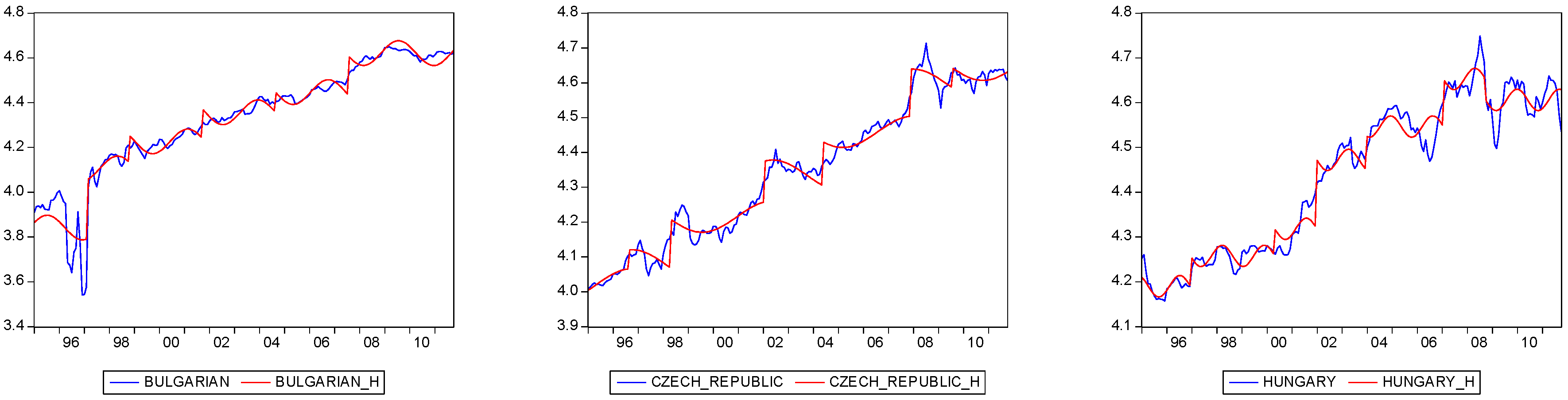
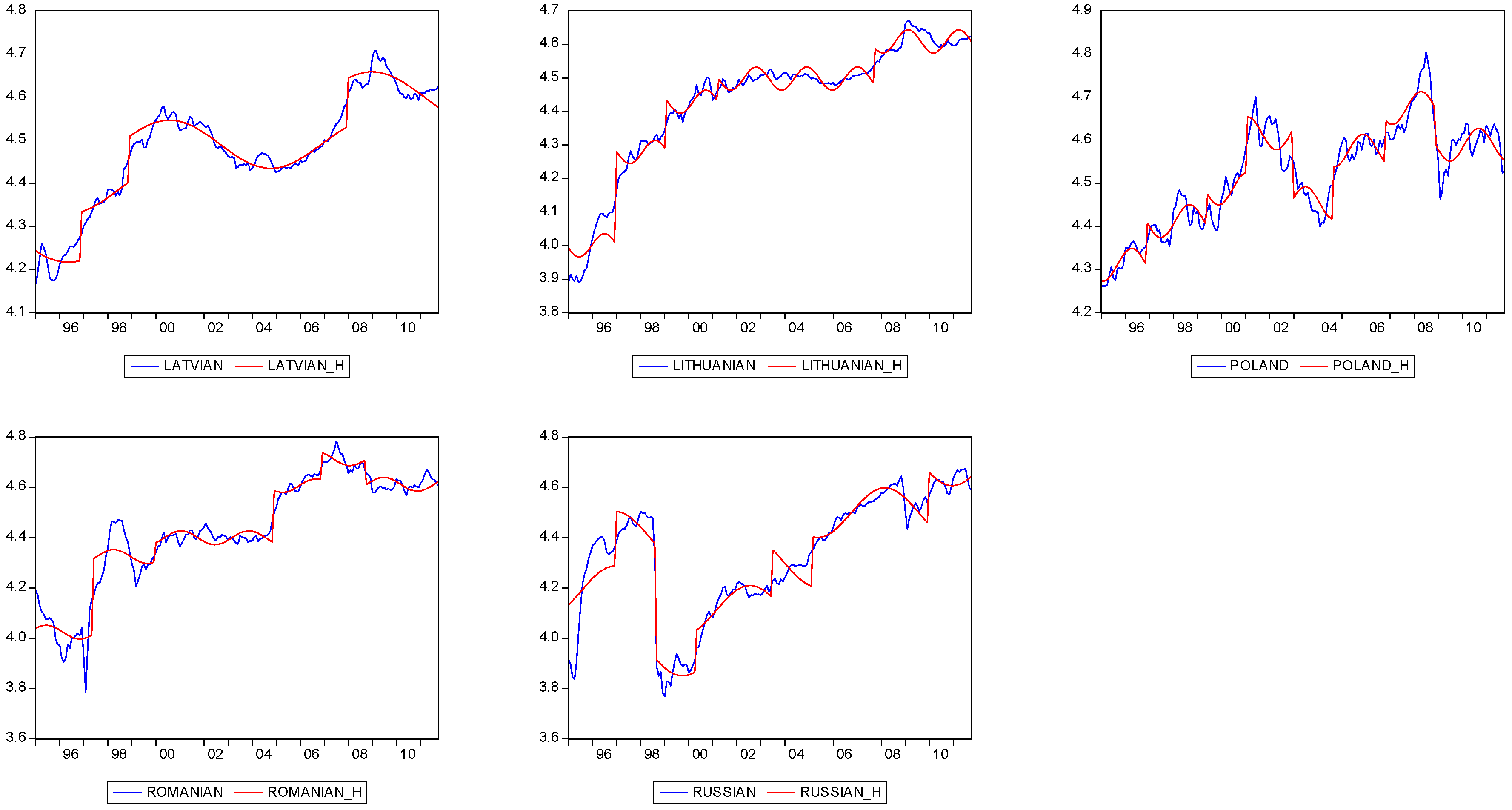
4. Empirical Results and Policy Implications

As a preliminary exercise, we first applied a few standard univariate tests, such as augmented Dickey-Fuller (ADF), PP (Phillips and Perron) and KPSS (Kwiatkowski, Phillips, Schmidt, Shin [8]) tests, to each country’s real exchange rate. The results appear in Table 1, where all three tests indicate that the real exchange rates are non-stationary for these eight transition countries, implying failure of the PPP. These results are consistent with that of existing literature and may be due to the low power of these three univariate unit root tests when the real exchange rates are highly persistent. 3

Next, we shift to Equation (3) and panel stationary tests with sharp shifts and smooth breaks and report the results in Table 2. 4 Following Bahmani-Oskooee et al. [4], we computed the critical values using Monte Carlo simulation and 5000 replications. From Table 2, we gather that according to our panel stationary tests results, the null hypothesis of stationarity is rejected for all of the countries, when both homogenous long-run variance and heterogeneous long-run variance are used. However, the results of the univariate stationary test indicate that the null of stationarity is not rejected for Lithuania and Poland at the 1% significant level. Based on these findings, we can conclude that this approach provides weak evidence of the long-run PPP in transition countries being studied. These results are consistent with those of Beko and Borsic [10] and Baharumshah and Borsic [11], who provided weak (or no) support for PPP for various groups of transition countries.

Our empirical results might originate from several factors, such as differences in technology/productivity and preferences, different factor endowments, trade barriers, transportation costs and differences in price index formations. It should also be noted that the share of government activities in these transition countries is still large, which makes the prices administrated. The administrated prices might be an important source of deviation from the PPP in these transition countries. Therefore, it is possible to claim that deviations in the short run form the PPP are prolonged for most of these transition countries, and there are no forces that are capable of bringing the exchange rate back to its PPP values in the long run.

Table 1. Univariate unit root tests. ADF, augmented Dickey-Fuller; PP, Phillips and Perron.

Countries	Level			1st Difference
	ADF	PP	KPSS	ADF	PP	KPSS
Bulgarian	−0.884(4)	−2.406(4)	1.597[11] ***	−10.11(1) ***	−41.03(4) ***	0.095[3]
Czech Republic	−0.742(0)	−0.742(1)	1.485[11] ***	−13.48(0) ***	−13.47(2) ***	0.087[1]
Hungary	−0.902(0)	−0.856(2)	1.366[11] ***	−14.10(0) ***	−14.12(2) ***	0.146[3]
Latvian	−1.497(0)	−1.505(4)	1.529[11] ***	−14.01(0) ***	−14.01(1) ***	0.107[3]
Lithuanian	−2.3337(0)	−2.156(4)	1.680[11] ***	−12.78(0) ***	−12.82(4) ***	0.321[5]
Poland	−1.734(0)	−1.746(1)	1.405[11] ***	−12.44(0) ***	−14.01(2) ***	0.042[2]
Romanian	−1.421(3)	−1.344(7)	1.467[11] ***	−6.11(2) ***	−10.73(5) ***	0.205[7]
Russian	−1.198(0)	−1.550(7)	0.875[11] ***	−11.25(0) ***	−11.46(6) ***	0.077[7]

Note: *** indicates significance at the 0.01; the numbers in parenthesis indicate the lag order selected based on the recursive t-statistic, as suggested by Perron [12]; the numbers in brackets indicate the truncation for the Bartlett kernel, as suggested by the Newey-West test [13].

Table 1. Univariate unit root tests. ADF, augmented Dickey-Fuller; PP, Phillips and Perron.

Countries	Level			1st Difference
	ADF	PP	KPSS	ADF	PP	KPSS
Bulgarian	−0.884(4)	−2.406(4)	1.597[11] ***	−10.11(1) ***	−41.03(4) ***	0.095[3]
Czech Republic	−0.742(0)	−0.742(1)	1.485[11] ***	−13.48(0) ***	−13.47(2) ***	0.087[1]
Hungary	−0.902(0)	−0.856(2)	1.366[11] ***	−14.10(0) ***	−14.12(2) ***	0.146[3]
Latvian	−1.497(0)	−1.505(4)	1.529[11] ***	−14.01(0) ***	−14.01(1) ***	0.107[3]
Lithuanian	−2.3337(0)	−2.156(4)	1.680[11] ***	−12.78(0) ***	−12.82(4) ***	0.321[5]
Poland	−1.734(0)	−1.746(1)	1.405[11] ***	−12.44(0) ***	−14.01(2) ***	0.042[2]
Romanian	−1.421(3)	−1.344(7)	1.467[11] ***	−6.11(2) ***	−10.73(5) ***	0.205[7]
Russian	−1.198(0)	−1.550(7)	0.875[11] ***	−11.25(0) ***	−11.46(6) ***	0.077[7]

Note: *** indicates significance at the 0.01; the numbers in parenthesis indicate the lag order selected based on the recursive t-statistic, as suggested by Perron [12]; the numbers in brackets indicate the truncation for the Bartlett kernel, as suggested by the Newey-West test [13].

Table 2. Panel stationary test with sharp and smooth breaks.

Panel A: Panel Stationary Test
Pesaran (2004) is cross-sectional dependence test			Test	p-Values
			31.568	0.000
Panel stationary test			Test	Critical values
				90	95	97.5	99
Homogenous long-run variance			2.648	1.386	2.212	2.993	4.084
Heterogeneous long-run variance			3.436	1.122	1.587	2.035	2.612
Panel B: Univariate Stationary Test
Countries	Bartlett	90%	95%	97.5%		99%
Bulgarian	0.0787	0.0741	0.0913	0.1073		0.1330
Czech Rep.	0.0421	0.0371	0.0425	0.0483		0.0545
Hungary	0.0481	0.0447	0.0516	0.0579		0.0698
Latvian	0.0471	0.0348	0.0401	0.0456		0.0534
Lithuanian	0.0471	0.0688	0.0836	0.0999		0.1160
Poland	0.0336	0.0339	0.0385	0.0436		0.0502
Romanian	0.0683	0.0349	0.0461	0.0540		0.0637
Russian	0.0486	0.0344	0.0387	0.0437		0.0491

Notes: The finite sample critical values are computed by a Monte Carlo simulation using 5000 replications; the maximum breaks and frequencies were fixed at 10, respectively.

Table 2. Panel stationary test with sharp and smooth breaks.

Panel A: Panel Stationary Test
Pesaran (2004) is cross-sectional dependence test			Test	p-Values
			31.568	0.000
Panel stationary test			Test	Critical values
				90	95	97.5	99
Homogenous long-run variance			2.648	1.386	2.212	2.993	4.084
Heterogeneous long-run variance			3.436	1.122	1.587	2.035	2.612
Panel B: Univariate Stationary Test
Countries	Bartlett	90%	95%	97.5%		99%
Bulgarian	0.0787	0.0741	0.0913	0.1073		0.1330
Czech Rep.	0.0421	0.0371	0.0425	0.0483		0.0545
Hungary	0.0481	0.0447	0.0516	0.0579		0.0698
Latvian	0.0471	0.0348	0.0401	0.0456		0.0534
Lithuanian	0.0471	0.0688	0.0836	0.0999		0.1160
Poland	0.0336	0.0339	0.0385	0.0436		0.0502
Romanian	0.0683	0.0349	0.0461	0.0540		0.0637
Russian	0.0486	0.0344	0.0387	0.0437		0.0491

Notes: The finite sample critical values are computed by a Monte Carlo simulation using 5000 replications; the maximum breaks and frequencies were fixed at 10, respectively.

Table 3. Estimation results for the mean reverting function in Equation (3).

Panel A: The Results for Optimum Frequency and the F-Statistic and Its Critical Values
Countries	Optimum Frequency	F stat	90%	95%	97.50%	99%
Bulgarian	5	23.805	2.005	2,797	2.999	3.031
Czech Rep.	8	22.203	2.196	2.598	2.995	3.442
Hungary	10	36.323	2.488	3.245	3.714	4.091
Latvian	4	33.934	1.941	2.693	3.716	3.951
Lithuanian	9	18.421	1.744	2.202	3.025	8.811
Poland	1	72.492	3.084	4.617	4.800	5.245
Romanian	8	35.406	2.300	2.540	3.215	3.407
Russian	6	62.527	2.135	2.375	3.374	4.601
Panel B: The Results for Sharp Drift Dates in Equation (3)
Countries	Break Dates
Bulgarian	02-1997	11-2001	10-2005
Czech Rep.	02-1997	03-1999	01-2002	10-2003	04-2006	01-2008
Hungary	06-1997	06-1999	04-2001	10-2002	03-2004
Latvian	09-1996	10-1996	06-2001	12-2002	02-2004	10-2005
Lithuanian	09-1996	06-2001	02-2002	10-2004
Poland	01-2000	08-2001	10-2002	03-2004	11-2005
Romanian	12-1996	12-1998	08-1999	04-2000	05-2004	11-2006
Russian	12-1996	06-1998	06-1999	02-2001	12-2003	03-2005

Table 3. Estimation results for the mean reverting function in Equation (3).

Panel A: The Results for Optimum Frequency and the F-Statistic and Its Critical Values
Countries	Optimum Frequency	F stat	90%	95%	97.50%	99%
Bulgarian	5	23.805	2.005	2,797	2.999	3.031
Czech Rep.	8	22.203	2.196	2.598	2.995	3.442
Hungary	10	36.323	2.488	3.245	3.714	4.091
Latvian	4	33.934	1.941	2.693	3.716	3.951
Lithuanian	9	18.421	1.744	2.202	3.025	8.811
Poland	1	72.492	3.084	4.617	4.800	5.245
Romanian	8	35.406	2.300	2.540	3.215	3.407
Russian	6	62.527	2.135	2.375	3.374	4.601
Panel B: The Results for Sharp Drift Dates in Equation (3)
Countries	Break Dates
Bulgarian	02-1997	11-2001	10-2005
Czech Rep.	02-1997	03-1999	01-2002	10-2003	04-2006	01-2008
Hungary	06-1997	06-1999	04-2001	10-2002	03-2004
Latvian	09-1996	10-1996	06-2001	12-2002	02-2004	10-2005
Lithuanian	09-1996	06-2001	02-2002	10-2004
Poland	01-2000	08-2001	10-2002	03-2004	11-2005
Romanian	12-1996	12-1998	08-1999	04-2000	05-2004	11-2006
Russian	12-1996	06-1998	06-1999	02-2001	12-2003	03-2005

Figure 1 displays the time paths of the real exchange rates where a positive change in the exchange rate indicates real depreciation. Structural breaks in the data are clear, and this justifies considering both sharp shifts and smooth breaks in testing for a unit root. The estimated time paths of the time-varying intercepts are also shown in all figures. The actual nature of break(s) is generally unknown, and there is no specific guide as to where and how many breaks to use in testing for a unit root or stationarity. A further examination of the figures indicates that both dummy variables and Fourier approximations seem reasonable and support the notion of long swings in real exchange rates. 5

Figure 1. Time series plot of real exchange rates (in log form) for eight transition countries and the fitted nonlinear flexible intercept with sharp shifts and smooth breaks.

Figure 1. Time series plot of real exchange rates (in log form) for eight transition countries and the fitted nonlinear flexible intercept with sharp shifts and smooth breaks.

5. Conclusions

In contrast to old studies, which tried to establish the long-run relation between the nominal exchange rate and relative prices, recent studies have combined the two variables into one and have investigated the mean reverting property of the new variable, i.e., the real exchange rate. If the real exchange rate reverts to its mean, it is said to have no unit root or it is stationary, supporting the purchasing power parity.

Since the introduction of unit-root tests, different authors have applied different test and have not provided uniform support for the theory. While some have applied a univariate unit-root test to an individual country’s data, some have relied upon panel models combining time-series across countries. The panel unit-root tests are said to enjoy more power due to the increased number of observations. It has been argued that regardless of the nature of the test, failure to account for structural break could result in misleading results. To that end, some have included dummy variables to reduce the biasness of the results. The difficulty of including a dummy is that one must know the exact break date.

In case there is more than one sharp break with an unknown date and some other smooth breaks, Bahmani-Oskooee et al. [4] proposed a new stationary test in the panel setting, which accounts for both sharp and smooth breaks. We apply this new approach for a sample of eight transition countries over the period of January 1995 to October 2011. While standard univariate or panel tests reject the PPP, the new test indicates that PPP is supported at least in two countries (i.e., Lithuania and Poland).

References

1. M. Bahmani-Oskooee, and S. Hegerty. “Purchasing power parity in less-developed and transition economies: A review article.” J. Econ. Surv. 23 (2009): 617–658. [Google Scholar] [CrossRef]
2. K.S. Im, M.H. Pesaran, and Y. Shin. “Testing for unit roots in heterogeneous panels.” J. Econom. 115 (2005): 53–74. [Google Scholar] [CrossRef]
3. W. Enders, and J. Lee. “A unit root test using a Fourier series to approximate smooth breaks.” Oxf. Bull. Econ. Stat. 74 (2012): 574–599. [Google Scholar] [CrossRef]
4. M. Bahmani-Oskooee, T. Chang, and T. Wu. “Revisiting purchasing power parity in African countries: Panel stationary test with sharp and smooth breaks.” Appl. Financ. Econ. 24 (2014): 1429–1438. [Google Scholar] [CrossRef]
5. W. Enders, and M.T. Holt. “Sharp breaks or smooth shifts? An investigation of the evolution of primary commodity prices.” Am. J. Agric. Econ. 94 (2012): 659–673. [Google Scholar] [CrossRef]
6. J. Bai, and P. Perron. “Estimating and testing linear models with multiple structural changes.” Econometrica 66 (1998): 47–78. [Google Scholar] [CrossRef]
7. J.L. Carrión-i-Silvestre, and A. Sansó. “A guide to the computation of stationarity tests.” Empir. Econ. 31 (2006): 433–448. [Google Scholar] [CrossRef]
8. D. Kwiatkowski, P.C.B. Phillips, P. Schmidt, and Y. Shin. “Testing the null hypothesis of stationarity against the alternative of a unit root: How sure are we that economic time series have a unit root? ” J. Econom. 54 (1992): 159–178. [Google Scholar] [CrossRef]
9. D.E. Rapach, and M.E. Wohar. “Testing the monetary model of exchange rate determination: A closer look at panels.” J. Int. Money Financ. 23 (2004): 867–895. [Google Scholar] [CrossRef]
10. J. Beko, and D. Borsic. “Purchasing power parit y in transition economics.” Post-Communist Econ. 19 (2007): 417–432. [Google Scholar] [CrossRef]
11. A.Z. Baharumshah, and D. Borsic. “Purchasing power parity in Central and Eastern European countries.” Econ. Bull. 6 (2008): 1–8. [Google Scholar]
12. P. Perron. “The great crash, the oil price shock, and the unit root hypothesis.” Econometrica 55 (1989): 277–302. [Google Scholar]
13. W. Newey, and K. West. “Automatic lag selection in covariance matrix estimation.” Rev. Econ. Stud. 61 (1994): 631–653. [Google Scholar] [CrossRef]
14. F.W. Ahking. “Testing long-run purchasing power parity with a Bayesian unit root approach: The experience of Canada in the 1950s.” Appl. Econ. 29 (1997): 813–819. [Google Scholar] [CrossRef]
15. N. Apergis. “Budget deficits and exchange rates: Further evidence from cointegration and causality Tests.” J. Econ. Stud. 25 (1998): 161–178. [Google Scholar] [CrossRef]
16. A.C. Arize, J. Malindretos, and S. Christoffersen. “Monetary dynamics, exchange rates and Parameter Instability: An empirical investigation.” J. Econ. Stud. 30 (2002): 493–513. [Google Scholar] [CrossRef]
17. J. Baffoe-Bonnie. “Dynamic modelling of faiscal and exchange rates policy effects in a developing country: A non-structural approach.” J. Econ. Stud. 31 (2004): 57–75. [Google Scholar] [CrossRef]
18. E.D. Beach, N.C. Kruse, and N.D. Uri. “The doctrine of relative purchasing power parity re-examined.” J. Econ. Stud. 20 (1993): 3–23. [Google Scholar] [CrossRef]
19. M. Bleaney. “Does Long-run purchasing-power parity hold within the European Monetary System? ” J. Econ. Stud. 19 (1992): 66–72. [Google Scholar] [CrossRef]
20. H. Bwo-Nung. “Long-run purchasing power parity revisited: A Monte Carlo simulation.” Appl. Econ. 28 (1996): 967–974. [Google Scholar] [CrossRef]
21. J.I. Carrion-I-Silvestre, T. del Barrio, and E. Lopez-Bazo. “Evidence on the purchasing power parity in a panel of cities.” Appl. Econ. 36 (2004): 961–966. [Google Scholar] [CrossRef]
22. W. Enders, and K. Chumrusphonlert. “Threshold Cointegration and Purchasing Power Parity in the Pacific Nations.” Appl. Econ. 36 (2004): 889–896. [Google Scholar] [CrossRef]
23. D.E. Hojman. “Fundamental equilibrium exchange rates under contractionary devaluation: A peruvian model.” J. Econ. Stud. 16 (1989): 5–26. [Google Scholar] [CrossRef]
24. M.J. Holmes. “Exchange rate regimes and economic convergence in the European Union.” J. Econ. Stud. 29 (2002): 6–20. [Google Scholar] [CrossRef]
25. J. Horne. “Eight conjectures about exchange rates.” J. Econ. Stud. 31 (2004): 524–548. [Google Scholar] [CrossRef]
26. M.A. Jenkins. “Purchasing power parity and the role of traded goods: Evidence from EU States.” Appl. Econ. 36 (2004): 1371–1375. [Google Scholar] [CrossRef]
27. C. Jung. “Forecasting of foreign exchange rate by normal mixture models.” J. Econ. Stud. 22 (1995): 45–57. [Google Scholar] [CrossRef]
28. G. Macdonals. “Purchasing power parity-evidence from a new panel test.” Appl. Econ. 34 (2002): 1319–1324. [Google Scholar] [CrossRef]
29. I.A. Moosa. “Testing proportionality, symmetry and exclusiveness in long-run PPP.” J. Econ. Stud. 21 (1994): 3–21. [Google Scholar] [CrossRef]
30. D.M. Nachane. “Purchasing power parity: An analysis based on the evolutionary spectrum.” Appl. Econ. 29 (1997): 1515–1524. [Google Scholar] [CrossRef]
31. P.K. Narayan. “New evidence on purchasing power parity from 17 OECD countries.” Appl. Econ. 37 (2005): 1063–1071. [Google Scholar] [CrossRef]
32. D.A. Peel, and I.A. Venetis. “Purchasing power parity over two centuries: Trends and nonlinearity.” Appl. Econ. 35 (2003): 609–617. [Google Scholar] [CrossRef]
33. P. Sjolander. “Unreal exchange rates: A simulation based approach to adjust misleading PPP estimates.” J. Econ. Stud. 34 (2007): 256–288. [Google Scholar] [CrossRef]
34. M.P. Taylor. “An empirical examination of long-run purchasing power parity using cointegration technique.” Appl. Econ. 20 (1988): 1369–1381. [Google Scholar] [CrossRef]
35. M.P. Taylor, D.A. Peel, and L. Sarno. “Nonlinear mean-reversion in real exchange rates: Toward a solution to the purchasing power parity puzzles.” Int. Econ. Rev. 42 (2001): 1015–1042. [Google Scholar] [CrossRef]
• 1Enders and Holt [5] is the first study that discusses sharp breaks or smooth shifts in investigating the evolution of primary commodity prices.
• 2The null hypothesis is that data are stationary, and the alternative hypothesis is that data are non-stationary.
• 3Following Rapach and Wohar [9], we calculate the half-life of a shock for each country, and it is based on using the cumulative impulse response function. We classify transition countries according to their half-lives into two groups; countries with a half-life less than one year (first group) and countries with a half-life less than two years (second group). The results of the half-life show that a shock to the real exchange rate of Bulgaria will dissipate by one-half in about 7.89 months. A shock to real exchange rates of the rest of the seven countries (i.e., Czech Republic, Hungary, Latvia, Lithuania, Poland, Romania and Russia) require a time period of 20 months for dissipating by one-half. Calculation of confidence intervals for the half-life shows that the confidence intervals are very wide for the half-life of all eight countries. The results show a high degree of persistence in the real exchange rate series.
• 4Maximum number of breaks and frequencies are fixed at 10 for each country. The optimum frequency and drift dates are reported in Table 3.
• 5For some other PPP and exchange rate-related studies, see [14,15,16,17,18,19,20,21,22,23,24,25,26,27,28,29,30,31,32,33,34,35].