On the Use of Local Search in the Evolution of Neural Networks for the Diagnosis of Breast Cancer

Abstract

With the advancement in the field of Artificial Intelligence, there have been considerable efforts to develop technologies for pattern recognition related to medical diagnosis. Artificial Neural Networks (ANNs), a significant piece of Artificial Intelligence forms the base for most of the marvels in the former field. However, ANNs face the problem of premature convergence at a local minimum and inability to set hyper-parameters (like the number of neurons, learning rate, etc.) while using Back Propagation Algorithm (BPA). In this paper, we have used the Genetic Algorithm (GA) for the evolution of the ANN, which overcomes the limitations of the BPA. Since GA alone cannot fit for a high-dimensional, complex and multi-modal optimization landscape of the ANN, BPA is used as a local search algorithm to aid the evolution. The contributions of GA and BPA in the resultant approach are adjudged to determine the magnitude of local search necessary for optimization, striking a clear balance between exploration and exploitation in the evolution. The algorithm was applied to deal with the problem of Breast Cancer diagnosis. Results showed that under optimal settings, hybrid algorithm performs better than BPA or GA alone.

1. Introduction

Computational tools are extensively used for medical diagnosis. These tools assist doctors in order to take decisions. Medical expert systems [1,2] largely rely on the availability of historical datasets recorded for diseased and non-diseased people. These tools are able to extract knowledge from the datasets and use the same knowledge to predict the likelihood of any disease. Doctors have limitations, which can easily be overcome by using such expert systems. These automated systems can often extract hidden knowledge and can interpret data that is not possible for doctors alone. Such systems are necessary for accurate diagnosis. Whereas a false positive outcome can lead to unnecessary treatment, thus risking the life of an individual, a false negative can lead to delayed treatment, jeopardizing the life of an individual. Therefore, accuracy in recognition techniques has become the primary requirement for such systems and, thus, a lot of effort is being put into developing efficient algorithms. Extracting efficient knowledge from the data provided in an optimal manner is the ultimate goal for these algorithms. Therefore, we attempt to develop an efficient recognition system that can provide beneficial results with less complexity, and is also robust.

Breast Cancer [3,4] has captured much interest from the research community due to its high fatality rate and widespread occurrence. According to the National Cancer Institute [5], 124.6 new cases were reported per 100,000 women per year, with 22.2 deaths per 100,000 women per year during 2007–2011. Statistics reveal that approximately 12.3% of women are diagnosed with breast cancer during their lifetime. Recently, people have become more and more aware of this disease. Even though Breast Cancer can be identified by symptoms (including swelling and lumps), often these symptoms may not be very obvious. Early detection of breast cancer significantly helps in providing timely treatment. However, the actual diagnosis of breast cancer is a tedious process and involves biopsy as well as other tests to determine the nature and extent of the disease. Furthermore, it can take a long time for the biopsy results to be determined and analyzed, and the results may not always be very clear. Upon positive diagnosis, patients may need to undergo surgery, radiation therapy, chemotherapy, and/or other specialized therapies.

An Artificial Neural Network (ANN) [6] is a computer system modeled with the human brain and nervous system as inspiration. Feeding training data to the ANN modifies the parameters of the network accordingly, and produces results with the minimum amount of error possible. ANNs give the computational ability to learn a given data set of inputs and outputs, and generalize the learning to a new set of unseen inputs. Multi-Layer Perceptron model is a widely used model for this purpose, as it consists of neurons connected in a layered fashion. The inputs are mapped to the outputs with the help of neurons in the network. Every neuron connection is associated with a weight, whose values are learned from a historical dataset, and symbolizes the learned and summarized representation of the data. A very common learning algorithm used for training the network is the Back Propagation Algorithm (BPA). BPA sets the internal parameters of the network, or the weights and biases, by propagating the error function to the minima. It does supervised learning of the training dataset, wherein both the inputs and outputs are provided and the mapping function between the inputs and outputs is learned.

The problem with BPA is that it can get stuck in a local minimum. BPA is a gradient-based approach, and the gradient at local minima is zero. It is possible to use a multi-starter version of the BPA, wherein the algorithm is restarted a number of times after convergence, and the best results are used. This algorithm is better at escaping local minimums. However, the problem with learning of ANN weights and biases is that they are highly dimensional, with hundreds of parameters and a complicated mapping function to learn. There exist far too many modalities, and the possibility of getting global optima in a short computational time is negligible. Furthermore, the BPA does not learn the hyper parameters like number of neurons, connections, number of hidden layers, etc.; on the contrary, it introduces a set of hyper-parameters, which must be optimally set for good performance. The setting or learning of the hyper-parameters in itself is a big problem.

Genetic Algorithm (GA) [7,8] is extensively used for the purpose of optimization, automated system design, etc. The algorithm imitates the natural evolution process and Darwin’s theory of survival of the fittest. A population pool of individuals is taken, each individual representing some solution to the problem. The population pool evolves over time, usually keeping the total size constant, by application of some specialized evolutionary operations such as inheritance, mutation, selection and crossover. The best and the fittest individuals survive in a generation, while the weaker ones die and are eliminated from the pool. Along with generations, individuals converge toward the global optima.

GA is a multi-population method, where multiple solutions are worked in parallel. Though generally slower than BPA-like gradient-based search algorithms, the algorithm generally converges to the global optima, escaping most local minimums. The algorithm is not too negatively affected by high modality or dimensionality. This motivates the use of GA for solving the problem of learning in the ANN, giving rise to evolutionary neural networks [9,10].

The problem with GA is that it may take a very long time to analyze a high dimensional search space with multiple modalities, in pursuit of convergence to the global minimum. An attempt to make the search process fast by appropriate parameter setting makes the convergence speed faster; however, it also increases the risk of convergence to a local minimum. The GA simultaneously attempts exploitation or convergence to a local minimum, and exploration in pursuit of finding the global minimum. The GA is not assisted by the gradient information, which is vital for fast convergence.

Local search is commonly applied to GA to assist it in the optimization process. The local search is fast to converge on a local minimum, however it rarely escapes the local minimum. The GA is slow in convergence, however it usually finds the global minimum. Hence, attempts are made to hybridize the two approaches in pursuit of timely converging to the global minimum. In the hybrid approach, the GA is largely responsible for the placement of the individuals on the search landscape and using the evolutionary operators for strategized movement of these individuals over time. Since the search space is too complex, the local search moves these individuals towards the local minimum. Even a few iterations of the local search are enough to place the individuals near the local minimum. This gives the GA a good indication of the fitness of the individuals and helps it to better coordinate between the individuals.

The paper is organized as follows. Section 2 discusses some related works. Section 3 discusses the neural network framework for problem solving. Section 4 discusses the evolutionary framework for ANN learning. Section 5 presents the use of local search in the neuro-evolutionary framework. Section 6 presents the results of the approach. Conclusions are given in Section 7.

2. Related Works

A lot of work has been done on ANN and GA in the past few decades and these are slowly becoming important topics to study in the field of machine learning due to their various applications in real life, especially medical diagnosis. Burke et al. [11] noted the use of Pathological Tumor-Node-Metastasis (pTNM) staging system for cancer diagnosis, which was not very accurate and was inflexible. Using area under the curve, different types of prediction algorithms were compared. Using just TNM variables, it was found that both BPA and probabilistic neural network were significantly better than the pTNM staging system. Furthermore, adding more prognostic factors increased the BPA accuracy over other predicting algorithms. In a related work, Kala et al. [12] studied different simple and hybrid classification models for the detection of breast cancer. The hybrid methods consisted of ensembles of neural networks, adaptive neuro-fuzzy inference systems and GA optimized neural networks. It was shown that the hybrid methods outperformed the base methods, while the different hybrid methods were competent with each other.

More interesting applications of GA with ANN are found in other domains. Khan et al. [13] proposed a number of technical indicators for BPA-based neural networks and GA-based neural networks for predicting stock prices. The results were compared, and it was found that GA-based ANN was much better. Qin [14] proposed a model that diagnosed any fault in a chemical reactor. The author used hybrid ANN with GA for this purpose. The proposed ANN model had a three-layered feed-forward architecture with two GA loops for training. Implementing this method on various chemical reactions showed its superiority over BPA. Liyan and Chunfu [15] also used ANN and GA to forecast the traffic accident death toll in China. After desired calculations, they found that BPA predicted more deaths than hybrid neural network using GA.

Ling et al. [16] proposed a variable structure of ANN. The network model had ANN with nodes in each layer connected to nodes in the other layer and a Network Switch Controller (NSC). There were switches included in every link of the two nodes. NSC controlled these switches to give variability to the ANN structure. Furthermore, this ANN was trained using GA. By testing this network on XOR problem and hand-written pattern recognition, it was found that this network was better than BPA. Banik et al. [17] proposed a model for forecasting rain in Bangladesh. They used hybrid neural model of ANN, Adaptive Neuro-Fuzzy Inference System (ANFIS) and GA, which predicted better than BPA alone. Arram et al. [18] proposed a neural model for spam detection in email. In order to optimize ANN, GA was used. There were 57 different input parameters for detecting spam-like character frequencies, sequence of capital letters, frequencies of specified keywords, etc. After testing the dataset, it was shown that the hybrid of ANN and GA had a better accuracy than ANN alone.

A number of interesting models specialized to specific areas of application have been proposed. In order to reduce traffic congestion, Kaur and Agrawal [19] made an adaptive traffic signal controller. The adaptive traffic signal controller used ANN, which took time as an input and returned the queue length (number of vehicles) as output, whereas GA gave optimal time for the green light and gradually decreased the queue length. In another interesting work, Lam and Leung [20] developed a device that interpreted digits and command given by users using a modified ANN and GA. In this, the recognized characters were digits 0–9, and there were three commands, backspace, return and space. The input parameters were graffiti representations of these characters. The technique has been used in sports as well. By diagnoses of player tactics and skill of the player and of the opponent player, one can prepare crucial strategies. Similarly Kala et al. [21] studied the problem of dividing the attributes in a multi-input medical diagnosis problem and selected the best set of features for classification. Mao et al. [22] proposed such a hybrid neural network with GA for table tennis, which was used in the 2008 Beijing Olympic Games.

Even though much work has been done in the use of GA for neural learning in a variety of real life problems, the methods have not been very commonly applied for medical diagnosis. The complexity of matching of inputs and outputs, and the high dimensionality of the data, challenges the use of GA alone for the problem. Local search as an aid to neuro-evolution has not been sufficiently studied in the literature. This paper aims to take a step forward in this direction, thus specializing the study to medical diagnosis.

3. Neural Networks

ANNs are the elementary blocks for the pattern recognition intelligence. Neurons are connected in a layered fashion forming the architecture of ANN. The first layer, or the input layer, is a passive layer where the inputs are fed into the system. The last layer is the output layer from where the outputs are collected from the system. There may be multiple hidden layers in between.

For simplicity, we assume that the ANN has a single hidden layer. More and more hidden layers tend to increase the variance too much, which results in a good generalization of the historical data, especially for the problems where the historical data is limited. Let there be I neurons in the input layer, H neurons in the hidden layer and O neurons in the output layer. We further assume that the ANN has a fully connected architecture and all neurons in a layer are connected to the ones in the preceding and the following layers. Each connection is associated with a weight. Let w¹_ij denote the weight between the ith neuron of the input layer to the jth neuron of the hidden layer. Let w²_ij denote the weight between the ith neuron of the hidden layer to the jth neuron of the output layer. Let b¹_i be the bias associated with the ith hidden layer neuron. Let b²_i be the bias associated with the ith output layer neuron.

Functioning of the ANN is implemented in three phases: training phase, validation phase and testing phase. First, the data is pre-processed and normalized. The normalized data is divided into training, validation and testing sets. The training part of the data is initially fed into the ANN and used to set the weights and biases. The hyper-parameters of the network are set manually. A large number of combinations of the hyper-parameters are tried with the aim of increasing the accuracy on the validation dataset. The final accuracy on the testing dataset is recorded and quoted.

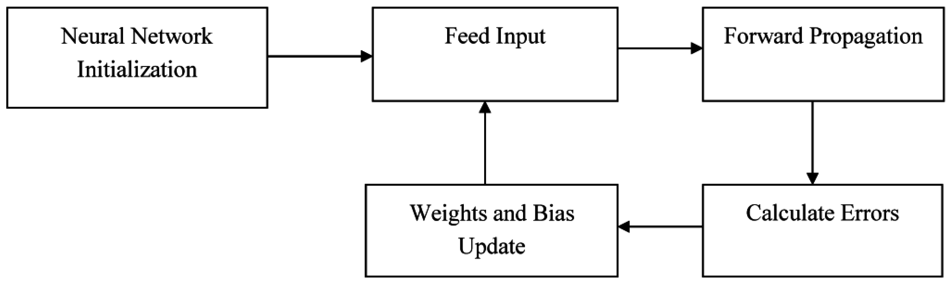
The training phase involves initialization, forward propagation and back propagation of learning. The general methodology is given in Figure 1. During testing, only forward propagation is applied to get the outputs from the supplied inputs.

During initialization, random bias values lying in the range [–1.0, 1.0] are assigned to each neuron in the hidden and output layer. Weights of the connections between the neurons are also assigned random values within the range [–1.0, 1.0]. The initialization of the network is shown in Algorithm 1.

Figure 1. Training of the neural network.

Figure 1. Training of the neural network.

Algorithm 1 Network_Initialization ()

for i from 1 to I

for j from 1 to H

w1ij = rand_between(–1, 1)

for i from 1 to H

for j from 1 to O

w2ij = rand_between(–1, 1)

for i from 1 to H, b1i = rand_between(–1, 1)

for i from 1 to O, b2j = rand_between(–1, 1)

Each input instance is fed to the neurons in the input layer. The hidden layer neurons take a weighted summation of the inputs, as shown in Equation (1). The weighted sum (z¹_i) so produced is then passed through an activation function to produce the outputs of the hidden layer (o¹_i), as shown in Equation (2). Sigmoid function is used as an activation function.

$$z_i^1=b_i^1+{\displaystyle {\sum }_{j=1}^I{w}_{ij}^1{x}_j}$$

(1)

$$o_i^1=\frac{1}{1+e^{-z_i^1}}$$

(2)

These outputs are fed into the output layer neurons, which again take the weighted sum of all the outputs (Equation (3)) and produce the final output on application of the activation function (Equation (4)).

$$z_i^2=b_i^2+{\displaystyle {\sum }_{j=1}^H{w}_{ij}^2{o}_j}$$

(3)

$$o_i^2=\frac{1}{1+e^{-z_i^2}}$$

(4)

The feed-forward phase of the ANN is given by Algorithm 2. Here, we calculate the input at a neuron and then the output is obtained from the neuron. Following this method for each neuron in the network, we calculate the final output of the network.

Algorithm 2 Feedforward

for i from 1 to H, Calculate o1i using Equations (1) and (2)

for i from 1 to O, Calculate o2i using equations (3) and (4)

BPA is implemented for the training of the network. The algorithm uses a gradient descent approach where gradient of the error function is calculated to compute the correction. The correction is propagated backward updating the bias values of the neurons and weights of the connections between the neurons. To measure the discrepancy between the actual output and the expected output, mean squared error function is implemented as given in Equation (5).

$$E=\frac{1}{2}{\left(t_j-o_j^2\right)}^2$$

(5)

where t_i is the expected output and o²_i is the actual output obtained from the network. The gradient of the error is given by Equations (6)–(8). The derivative of the error is given by Equation (6)

$$e_j^2=\frac{\partial E}{\partial o_j^2}=-\left(t_j-o_j^2\right)$$

(6)

For any general layer in the network, the derivative of the error, denoted by δ_j, is given by Equations (7)–(9).

$${\delta }_j=\frac{\partial E}{\partial z_j}=\frac{d{o}_j}{d{z}_j}\frac{\partial E}{\partial o_j}=o_j(1-o_j)\frac{\partial E}{\partial o_j}$$

(7)

$$\frac{\partial E}{\partial o_i}={\displaystyle \sum _j\frac{d{z}_j}{d{o}_i}\frac{\partial E}{\partial z_j}}={\displaystyle \sum _j{w}_{ij}\frac{\partial E}{\partial z_j}}={\displaystyle \sum _j{w}_{ij}{\delta }_j}$$

(8)

$$\frac{\partial E}{\partial w_{ij}}=\frac{\partial z_j}{\partial w_{ij}}\frac{\partial E}{\partial z_j}=o_i\frac{\partial E}{\partial z_j}=o_i{\delta }_j$$

(9)

The correction in weights of ANN is made proportional to the derivative of the error as per the gradient descent rule. The gradient descend rule can make the algorithm converge to a local minimum and converge very slowly. Hence, an additional term called momentum is added in the weight update equation, which attempts to make the weight update grow in the same direction as was done previously. The weight update is given by Equation (10).

$$w_{ij}^{new}=w_{ij}^{old}+\eta \frac{\partial E}{\partial w_{ij}}+\alpha \mathrm{\Delta }{w}_{ij}^{old}$$

(10)

where η is the learning rate whose value is set between 0 and 1. A very small value causes a very slow convergence to the local minimum, however the error at convergence is small. A very high value makes the system converge rapidly at the local minimum, while the system shows oscillations with high error on convergence. Escaping local minimum is very likely to occur with large values of learning rate. Similarly, momentum is usually kept between 0 and 1. Where a high value encourages fast convergence to the minimum at the risk of escaping the minimum, a low value contributes nothing worthy in the ANN training.

While using these equations, the bias term may be treated as a normal weight with a constant input of 1 and weight corresponding to the value of the bias. The equations involving bias can hence be easily derived.

The training of the 2-layer ANN using the general Equations (5)–(8) is given in Algorithm 3.

Algorithm 3 Train

//Calculate derivates for j from 1 to O, Calculate e2j for output layer using Equation (6) for j from 1 to O, δ2j = o2j (1 – o2j) e2j for i from 1 to H, e1i = ∑j(w2ijδ2j) for j from 1 to H, δ1j = o1j (1 – o1j) e1j //Adjust Weights and Biases for hidden to output layer for i from 1 to O   b2i ← b2i + η δ2i + α Δb2,oldi   Δb2,oldi ← η δ2i for i from 1 to H   for j from 1 to O     w2ij ← w2ij + η δ2jo2i + α Δδ2,oldj     Δδ2,°ldj ← η δ2jo2i //Adjust Weights and Biases for input to hidden layer for i from 1 to H   b1i ← b1i + η δ1i + α Δb1,oldi   Δb1,oldi ← η δ1i for i from 1 to I   for j from 1 to H     w1ij ← w1ij + η δ1jo1i + α Δwoldij     Δwoldij ← η δ1jo1i

In the validation stage, the network is trained for a variety of settings of the hyper-parameters, which includes the number of neurons (H), learning rate (η) and momentum (α). Different combinations of the hyper-parameters are tried. The aim is to get the settings of hyper-parameters, which give the best results on the validation data set. The optimal settings are noted. The trained ANN is then passed through the testing data set. This is the resultant accuracy of the system.

4. Evolution of Neural Networks

The greatest problem with the BPA is that it is bound to get stuck at the local minimum in problems where the optimization landscape is overly complicated with too many modalities. Momentum helps to some extent in escaping the local minimum. Restarting the process multiple times helps to mine out some of the possible local minimum with significantly larger computational time. However, such methods cannot be used in problems where the mapping between the inputs and outputs is highly complex and highly dimensional, wherein the modalities are very large. An associated problem with the BPA is that the performance is highly dependent on the settings of the hyper-parameters. The hyper-parameters are needed to be set manually and the chances of sub-optimality due to inherent limitations are very high.

A hybrid of GA and BPA is used to train the ANN. The GA maintains a population pool of individuals, each of which is a prospective solution to the problem. Each individual constituted in the population pool is associated with a fitness value, which is the goodness of the individual to solve the problem, and indicates the likelihood of survival of the individual after performing the evolutionary operations.

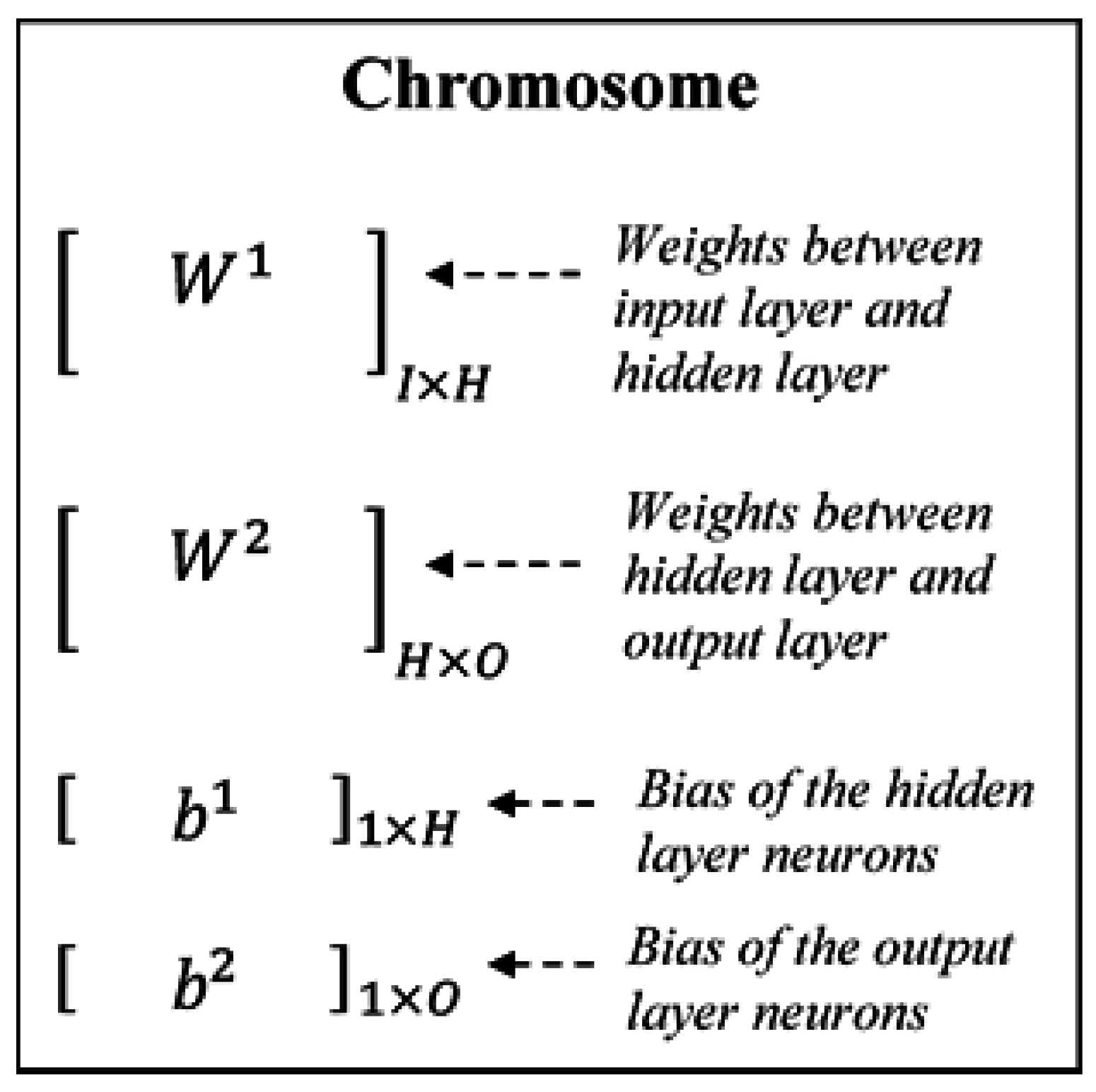
Here the problem is evolution of the ANN and hence every chromosome is an ANN encoded in a manner to ease the evolutionary process. The chromosome consists of the whole ANN with internal parameters. Constant parameters are not encoded, as they do not need to be optimized. Carrying the discussions from Section 3, a three-layered ANN is taken with an input layer, a hidden layer and an output layer, and fixed maximum number of neurons in the hidden layer (H). The number of neurons in the input layer (I) and output layer (O) are fixed for any system. The encoding is given in Figure 2. The encoding represents the weights between all the layers and the corresponding bias. The encoding is supplemented with the fitness value of the ANN, which is taken as the mean square error.

Figure 2. Structure of a chromosome.

Figure 2. Structure of a chromosome.

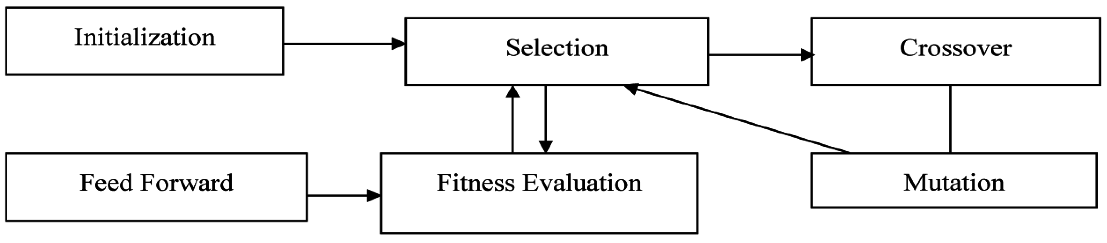
The general methodology working of GA is shown in Figure 3. First, random chromosomes are generated, which constitute the population pool. Then, individuals are selected from the pool to create individuals for the next generation. The fitter or more valued individuals are more likely to be selected. The individuals go through the evolutionary operators of crossover and mutation to build the next generation.

Figure 3. Working of Evolutionary Neural Network.

Figure 3. Working of Evolutionary Neural Network.

The process of initialization creates random chromosomes as the initial population pool. The total size of the population pool is kept constant. The pseudo code for initialization is given by Algorithm 4.

Algorithm 4 Initialization of population pool

population ← NIL for k from 1 to POOL_SIZE   for i from 1 to I     for j from 1 to H       chromosomek.w1ij = random_between(−1,1)   for i from 1 to H     for j from 1 to O       chromosomek.w2ij = random_between(−1,1)   for i from 1 to H, chromosomek.b1i = random_between(−1,1)   for i from 1 to O, chromosomek.b2i = random_between(−1,1) population ← population ∪ chromosomek

Selection is the process of stochastically selecting the individuals from the population pool. We have to select the best individuals representing ANN from the population pool, which is based on the fitness value of the network. The fewer errors there are, the better the network is and the more likely it will be selected. The selected individuals undergo certain genetic operations.

The individuals represent a real-valued encoding of the problem. The process of crossover takes two parents and creates two children by the exchange of characteristics from the parents. In real valued GA, the children must be generated in-between the parents so as to make the algorithm converge. Consequently, the weights and biases of the connections are altered by using genetic crossover. Consider two real-valued parents as x = (x₁,...,x_n) and y = (y₁,...,y_n). Let the two children generated be o¹ and o². The generation of children is such that the ith gene of the two children is given by Equations (11) and (12).

$$o_i^1=\beta y_i+\left(1-\beta \right)x_i$$

(11)

$$o_i^2=\left(1-\beta \right)y_i+\beta x_i$$

(12)

where β is a random number chosen between 0 and 1. The pseudo-code of crossover is given by Algorithm 5.

Algorithm 5 Crossover

children ← NIL for all pairs individual pairs x and y for crossover   for i from 1 to I     for j from 1 to H       β = rand_between(0, 1)       o1.w1ij = β × x.w1ij + (1 − β) × y.w1ij       o2.w1ij = (1 − β) × x.w1ij + β × y.w1ij   for i from 1 to H     for j from 1 to O       β = rand_between(0, 1)       o1.w2ij = β × x.w2ij + (1 − β) × y.w2ij       o2.w2ij = (1 − β) × x.w2ij + β × y.w2ij   for i from 1 to H     o1.b1i = β × x.b1i + (1 − β) × y.b1i     o2.b1i = (1 − β) × x.b1i + β × y.b1i   for i from 1 to O     o1.b2i = β × x.b2i + (1 − β) × y.b2i     o2.b2i = (1 − β) × x.b2i + β × y.b2i children ← children ∪ {o1,o2}

The next major evolutionary operator is mutation. Mutation attempts to move the individuals by small magnitudes in a fitness landscape, so as to explore the fitness landscape and reach towards the global minimum. Mutation modifies the internal parameters of the network in pursuit of increasing the precision and accuracy of the network. The genetic operator takes an individual and produces a child in the close vicinity. A Gaussian mutation is implemented, in which the magnitude of displacement is given by a Gaussian random number given in Equation (13).

$$f\left(x\right)=\frac{1}{\sigma \sqrt{2\pi }}{e}^{-\frac{{\left(x-\mu \right)}^2}{2{\sigma }^2}}$$

(13)

where σ is the standard deviation of the distribution and controls the magnitude by which individuals normally move in the fitness landscape. μ is the mean around which the random numbers are generated. Here, the mean is taken to be 0. The mutation is applied to all the weights and biases represented in the chromosome. The pseudo-code for mutation of chromosome x is given in Algorithm 6.

Algorithm 6 Mutation

for i from 1 to I   for j from 1 to H     r ← random Gaussian number with mean 0 and deviation σ     o1.w1ij ← x.w1ij + r     o1.w1ij ← MIN(o1.w1ij, 1), o1.w1ij ← MAX(o1.w1ij, −1) for i from 1 to H   for j from 1 to O     r ← random Gaussian number with mean 0 and deviation σ     o1.w2ij ← x.w2ij + r     o1.w2ij ← MIN(o1.w2ij, 1), o1.w2ij ← MAX(o1.w2ij, −1) for i from 1 to H   r ← random Gaussian number with mean 0 and deviation σ   o1.b1i ← x.b1i + r   o1.b1i← MIN(o1. b1i, 1), o1. b1i ← MAX(o1. b1i, −1) for i from 1 to O   r ← random Gaussian number with mean 0 and deviation σ   o1.b2i ← x.b2i + r   o1. b2i← MIN(o1. b2i, 1), o1. b1i ← MAX(o1. b2i, −1)

5. Local Search in Neuro-Evolution

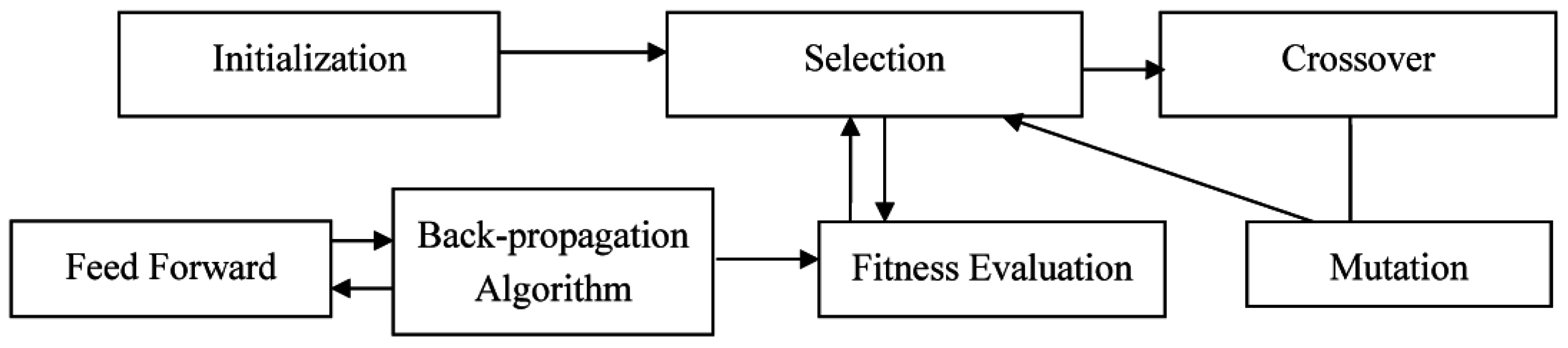
While GA can solve the inherent problems in BPA, the approach becomes very troublesome when the modality of the problem is too high, that is, it has too many local minimums. Exploitative settings of the algorithm result in fast convergence of the algorithm, however the chances of converging at a local minimum are very high. The explorative settings of the parameters make the algorithm search for global minimum, however the convergence is very slow. For a highly dimensional problem like neuro-evolution, it can take a significantly long amount of time. The BPA, on the other hand, shows a very fast convergence, which is also attributed to the use of the gradient of the error function. The purpose of this section is to fuse the two techniques and create a hybrid algorithm.

A small local search becomes very useful for the GA. The local search can quickly make the individual go near to its local minimum, to get a fair overall view of the fitness landscape. The GA is then largely responsible for the macroscopic search of the individuals in the fitness landscape, while the local search pushes all individuals to the nearest local minimum. The local searches are very fast and a few iterations of these searches takes much less time and results in a big improvement in the fitness value.

In the proposed approach, BPA is used as a local search operation for the GA. Every individual of the GA undergoes a few iterations of BPA before genetic operators are applied to it. Since BPA uses a gradient descent approach, the error are rapidly reduced in the first few iterations, enough to give a fair estimate to the GA regarding the expected fitness value. The resultant approach is summarized in Figure 4.

Figure 4. Working of Evolutionary Neural Network with Local Search.

Figure 4. Working of Evolutionary Neural Network with Local Search.

The BPA is applied once per generation. Hence, the BPA is integrated with the fitness function computation. We train the ANN in each chromosome using the same feed forward algorithm and make it learn using BPA. Fitness value is taken as the mean squared error, which is the error function of the ANN. The BPA is applied for L number of times, which is an algorithm parameter. In every iteration, the dataset is fed into the ANN, errors are computed, and the weights and biases are adjusted. The error during the last run of every instance is taken as the fitness value. The pseudo code of the local search and fitness evaluation is given as Algorithm 7.

Algorithm 7: Local Search
for every chromosomek in genetic population   for i from 0 to L     for every instance in the data set       train_and_backpropagate(chromosomek) chromosomek.fitness ← mean square error (dataset)

L, denoting the number of BPA iterations, is an algorithm parameter, which controls the relative contributions of the GA and BPA in the hybrid approach. Too large a value of this parameter resembles the multi-starter BPA approach with GA having virtually no inputs. Since the BPA will take a long time, the generations of GA would be kept at a minimum. Similarly, too small a value of this parameter makes the hybrid approach take no contributions from the BPA. It is equivalent to a global GA search. As the BPA has the largest gradient and correction at the initial iterations, the value of this parameter may be kept reasonably low, so as to contribute enough, while not taking excessive computational time.

6. Results

The system was simulated on the Breast Cancer Dataset from the UCI machine learning repository [23,24,25]. The dataset consists of nine real valued inputs. The inputs corresponds to the following attributes: clump thickness, uniformity of cell shape/size, marginal adhesion, single epithelial cell size, bare nuclei, bland chromatin, normal nucleoli and mitoses. There are a total of 583 data instances in the dataset. Each data instance is to be classified as malignant (unsafe) or benign (safe). The nine attributes were available from real world data, so it consisted of all the characteristics needed for the diagnosis of breast cancer in a patient. These values map to the following characteristics of each cell nucleus: radius (mean of distances from center to points on the perimeter), texture (standard deviation of gray-scale values), perimeter, area, smoothness (local variation in radius lengths), compactness (mathematically, perimeter²/area-1.0), concavity (severity of concave portions of the contour), concave points (number of concave portions of the contour), symmetry and fractal dimension (coastline approximation).

For the simulation, the dataset was divided into three different sets: training set (300 instances of 583 total instances, 51.45%), validation set (120 instances of 583 total instances, 20.58%) and testing set (163 instances of 583 total instances, 27.97%). The inputs were normalized. After normalization, each instance was fed to the developed ANN. The magnitude of data reserved for training is enough to capture all trends in the data set, considering that the problem is relatively simple with a simple decision boundary, indicated by the relatively small number of neurons in the hidden layer. Similarly, the magnitude of data reserved for testing is enough to give a high resolution of accuracy and minimize the effects of outliers. Therefore, the magnitude of data for this problem is not a limitation. Of course, if the dataset were small, we would have tried cross-validation.

6.1. Results and Comparisons with Back-Propagation Algorithm

The system was trained against a large number of combinations of hyper-parameters. The trends of accuracy, convergence and computational time were used to set the hyper-parameters. The intent was to maximize the performance on the validation data in acceptable computational times. The results corresponding to the best performance of the system on the validation dataset are presented. Since the number of hyper-parameters are very large, the ANN hyper-parameters were set using simulations on BPA only. Then, only the GA hyper-parameters were tuned. All the hyper-parameters were then separately analyzed.

The ANN had 19 neurons in total with nine neurons in the input layer, nine neurons in the hidden layer and one neuron in the output layer. GA operated for 50 generations with 11 individuals. BPA was used as a local search for a total of three iterations. The learning rate was set at 0.2 and momentum was set at 0.1.

The proposed method was compared with a standalone implementation of the ANN working with BPA alone. In order to make the comparisons realistic, the same architecture and hyper-parameters of the ANN were kept, as was the case with GA learning.

Results obtained from the two systems have been summarized in Table 1. The results presented are averaged over 50 independent runs. Noticeable accuracy was obtained. The GA took 2.723 s for execution, which is considerably shorter, keeping in mind the large data set and complex computations. It can be clearly seen that ANN with GA outperformed a conventional implementation of ANN with BPA alone.

Table 1. Comparative Analysis of the proposed work with Artificial Neural Network (ANN) and Back Propagation Algorithm (BPA).

Models	Type	Accuracy (%)	Standard Deviation
Evolutionary Neural Network	Validation	97.500	-
	Testing	99.579	0.314
Neural Network	Validation	96.217	-
	Testing	97.202	0.584

Table 1. Comparative Analysis of the proposed work with Artificial Neural Network (ANN) and Back Propagation Algorithm (BPA).

Models	Type	Accuracy (%)	Standard Deviation
Evolutionary Neural Network	Validation	97.500	-
	Testing	99.579	0.314
Neural Network	Validation	96.217	-
	Testing	97.202	0.584

6.2. Analysis of Neural Network Hyper-Parameters

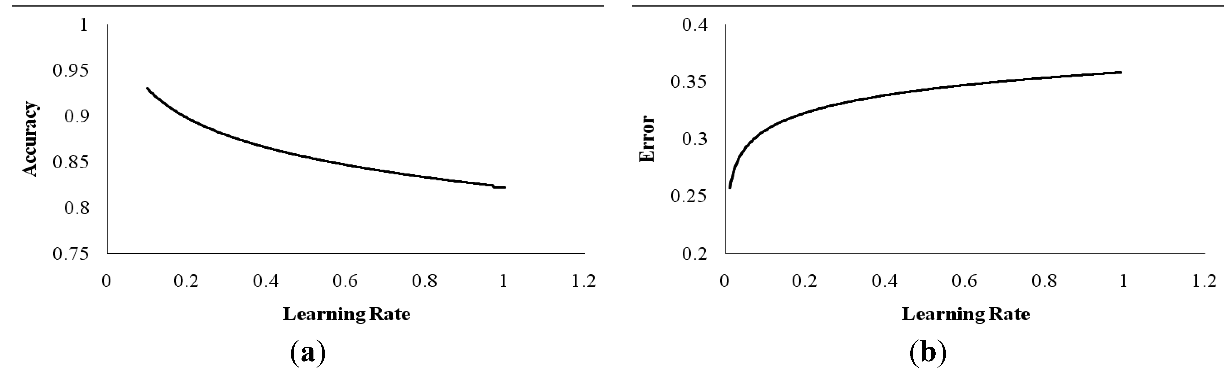
BPA is used as the learning algorithm for the training of ANN. BPA has numerous hyper-parameters whose settings severely affect the working of the overall algorithm. In this section, the various hyper-parameters are analyzed in order to get to a near-optimal setting. Learning Rate (η) describes the extent of correction applied at a unit iteration of the BPA. The larger is the step, the quicker is the convergence to a local minimum, while risking oscillations of large magnitude near the local minimum. Furthermore, the smaller is the step, the slower is the convergence with negligible oscillations. Ranging learning rate from 0.1 to 1.0 in increments of 0.1, the accuracy of the ANN is calculated and is plotted in Figure 5a. The series has been plotted as a trend line to better visualize the trends and minimize the noise due to randomness of the algorithm. Initially, the learning rate is 1, providing an accuracy of approximately 80%. With a decrease in learning rate, there was an increase in the accuracy of the ANN.

Error is inversely proportional to the accuracy. So, the behavior of error is opposite to that of the accuracy when the learning rate of the BPA is varied in the range of 0.1 to 1. The values obtained are plotted in Figure 5b. The figure is plotted as a trend line.

6.3. Analysis of Genetic Algorithm Hyper-Parameters

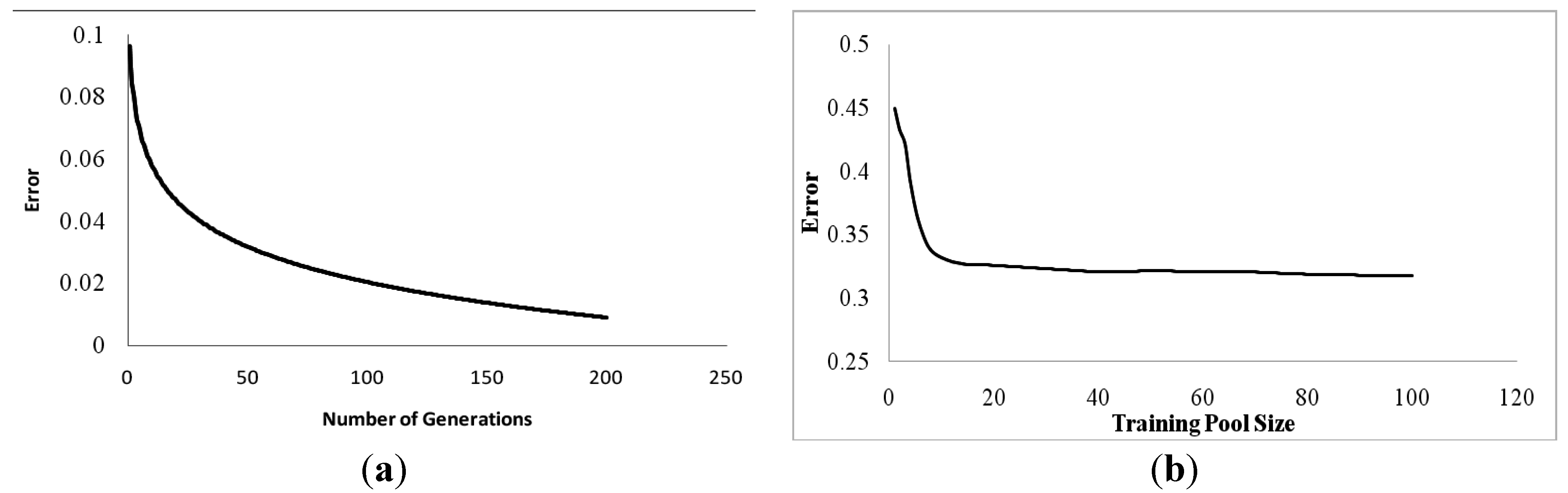
In comparison to simple ANN, the error is much less by using GA along with BPA. The hyper-parameters of both ANN and GA were analyzed in order to get the best parameter settings. Evolution needs time. The training accuracy improves with the application of mutation, selection, crossover and selection at every generation. Genes get transferred from ancestors to successors and a number of generations come into existence before the best individual is obtained. By selecting the best ANNs of each generation and evolving them further till the error function reaches global minimum, the evolutionary algorithms decrease the error to a large extent. The larger is the number of generations, the better is the evolved ANN and consequently the lesser is the error. The results of varying the number of generations and its effects on the error obtained have been plotted as a trend line in Figure 6a.

Figure 5. (a) Accuracy vs. Learning Rate. (b) Error vs. Learning Rate.

Figure 5. (a) Accuracy vs. Learning Rate. (b) Error vs. Learning Rate.

The larger is the size of the gene pool, the larger is the diversity in the population pool. The process of mutation increases the diversity of the genes in the search space and the process of crossover fuses the gene characteristics from different individuals to obtain new individuals with better characteristics. With an increase in the number of individuals, the error decreases up to a point but the computational complexity increases. At this point, further increase in the pool size has negligible effect on the error accounted. For different pool sizes, the error obtained is calculated and is plotted in Figure 6b.

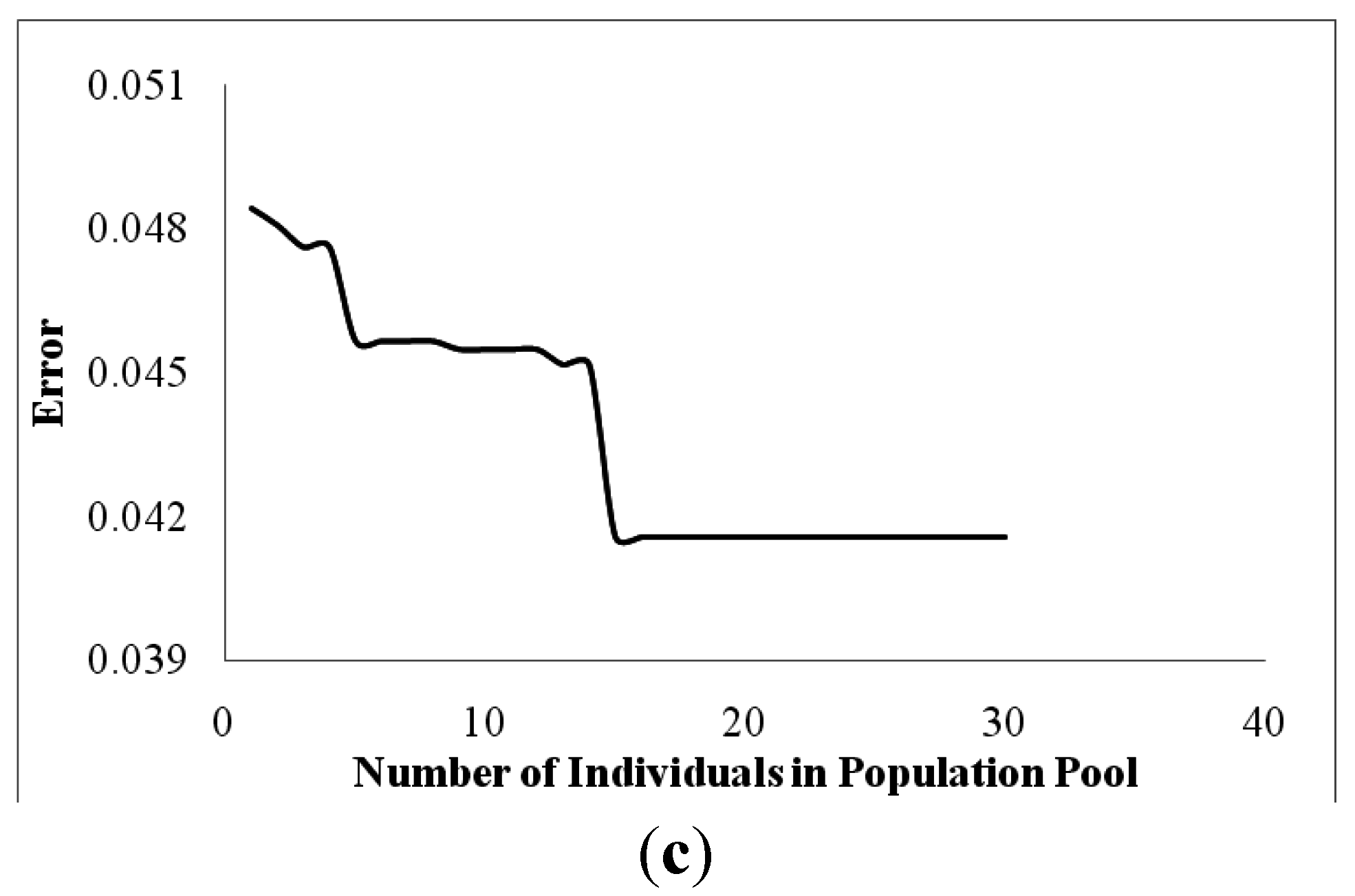
The lesser is the number of individuals, the lesser is the diversity. Increasing the number of individuals inversely affects the error accounted. We started with only two individuals in a gene pool and gradually increased the number till it reached 30. A huge decrease in error was accounted with an increase in the number of individuals. When the number of individuals in the population reached 20, negligible effect on error was accounted on further increment, because the pool was enough to explore the global optima. The effect of the number of the individuals on error accounted has been plotted in Figure 6c.

Figure 6. (a) Error vs. Number of Generations. (b) Error vs. Training Pool Size. (c) Error Accounted vs. Number of Individuals in the Population Pool.

Figure 6. (a) Error vs. Number of Generations. (b) Error vs. Training Pool Size. (c) Error Accounted vs. Number of Individuals in the Population Pool.

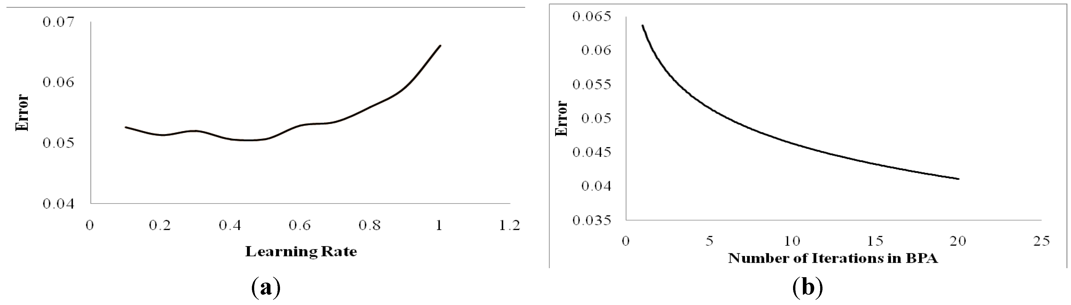
Next are the parameters of BPA, which was used as a local search. The first parameter is the learning rate (η) of the BPA used as a local search. As η increases the error also increases as shown in Figure 5a. But this time, the error is considerably less, as plotted in Figure 7a. Training the network modifies the weights and the biases in such a way that if a new input is fed into the network, the expected output is obtained. Starting with an iteration of the training loop and increasing it gradually to 20, a considerable amount of error reduction is observed. Training the network means propagating the error function to the minimum. Even though the training error reduces on increasing the number of iterations, prolonged training can lead to a large validation and testing error due to over-fitting. The results of error are plotted in Figure 7b.

Figure 7. (a) Error vs. Learning Rate. (b) Error vs. Number of iterations in BPA.

Figure 7. (a) Error vs. Learning Rate. (b) Error vs. Number of iterations in BPA.

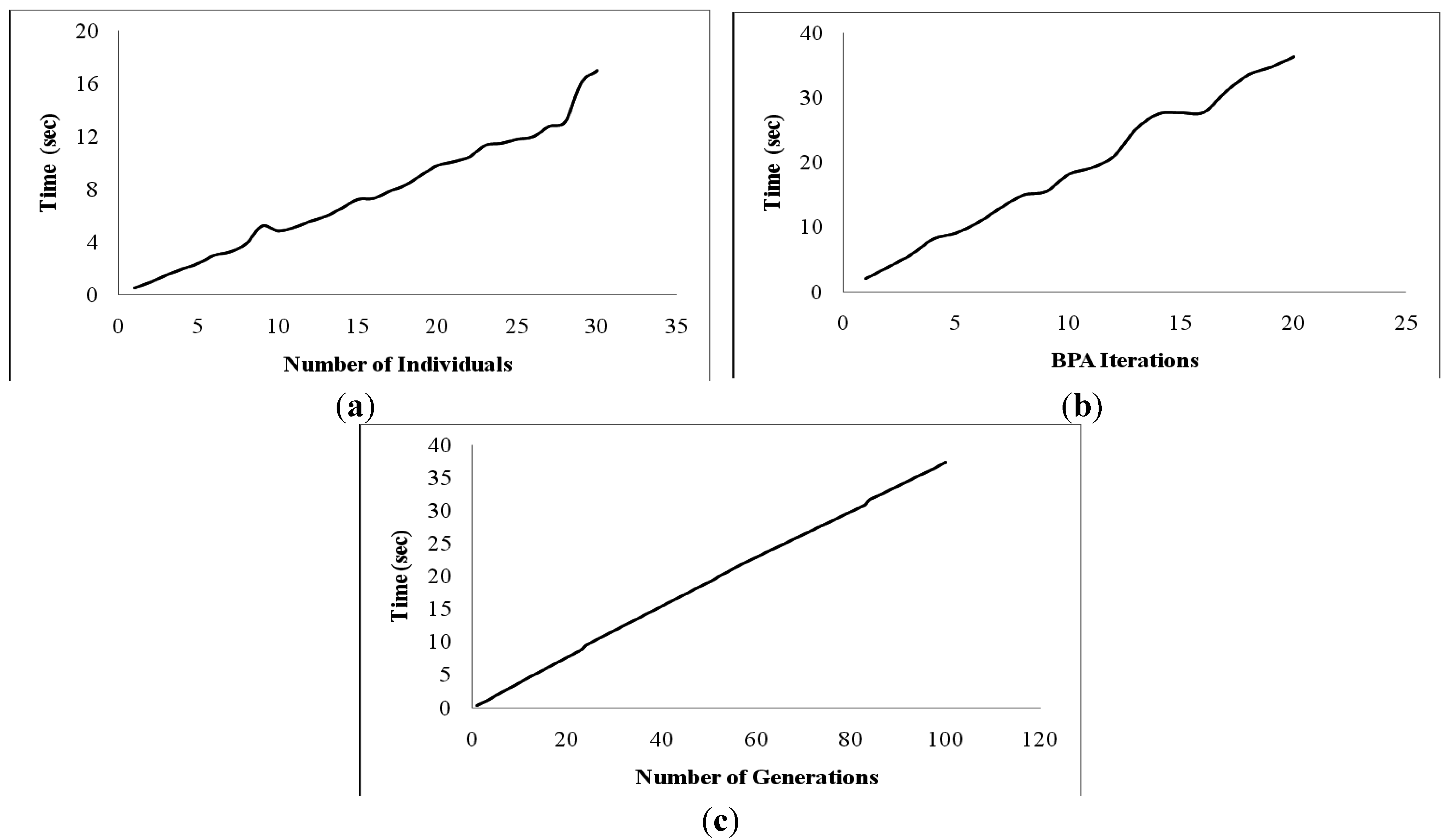
The current scenario demands algorithms, which take less time and produce notable results. Time is a huge factor in determining the efficiency of the algorithms. We have plotted the time spent in executing the algorithm for different number of individuals in the gene pool in Figure 8a, for different number of BPA iterations in Figure 8b, and for different number of generations in Figure 8c. Larger number of individuals, number of iterations of BPA and number of generations result in more computations and thus more time in the execution of the algorithm. Hence, even though the error is reduced with an increase of these parameters, the increase in computational time restricts their setting to very high values.

Figure 8. (a) Time vs. Number of individuals. (b) Time vs. BPA Iterations. (c) Time vs. Number of generations

Figure 8. (a) Time vs. Number of individuals. (b) Time vs. BPA Iterations. (c) Time vs. Number of generations

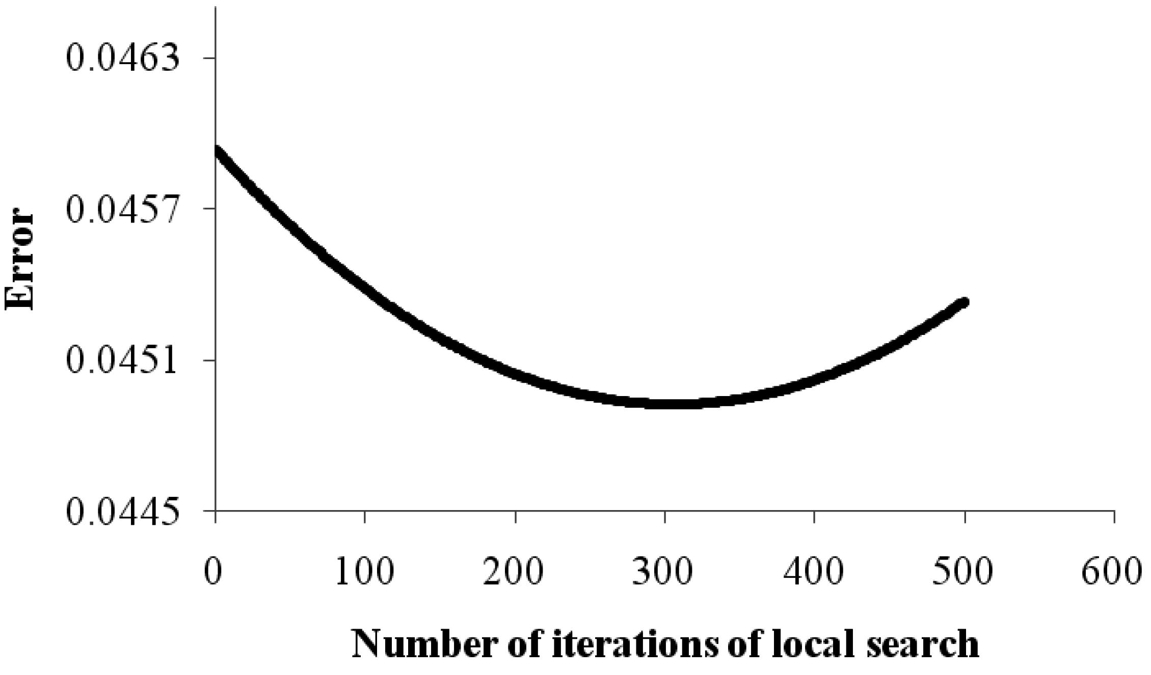
6.4. Effect of Local Search in Evolution

The aim of the paper was to study the effect of local optimization in the evolutionary process. While it is apparent that increase in the number of GA iterations (generations) and increase in the number of local search (BPA) iterations would both result in reduction in the training error, thus the individual components of both of these needs to be studied. Computational time is a big concern that limits the magnitude of training that can be performed. Hence, experiments were done keeping the computational time constant and changing the number of iterations of local search and GA. It is difficult to keep the computational time constant, and hence the total number of times the data set was fed for learning was taken as an indicator of the computational time. We allowed the algorithm to process the dataset for a fixed number of times, which for this process is given by the product of the number of BPA iterations, the number of GA iterations and the number of individuals. Keeping the number of individuals constant, we increase the number of local search iterations and decrease the number of generations such that the total computational time or the total number of times that the dataset is processed is constant. The results are recorded for a variety of readings. The results are plotted as a trend line to minimize the noise due to randomness and to better visualize the trends. The results are given in Figure 9. It is clear that neither GA nor BPA alone is good enough, considering the complicated and multi-modal optimization landscape. The hybrid approach gives the best results.

Figure 9. The effect of local search in overall optimization.

Figure 9. The effect of local search in overall optimization.

7. Conclusions

Considering the fatality of diseases, it is important to engineer solutions for automated diagnosis of patients. Historical medical records can be used as a means to engineer such solutions. ANNs have the capability to solve problems with high dimensionality. They can be trained like humans for cases where we know the output, and this training can be used for obtaining the solutions for cases where we do not know the output. The human brain attains a high level of intelligence with time by going through supervised and unsupervised learning through a series of actions and by sending electrical messages to every single connected neuron in the brain. BPA has a tendency of premature convergence to a local minimum, which leads to lower accuracy. We can avoid this premature convergence with the help of evolutionary operators.

In this paper, GA was used to improve upon the limitations of the conventional neural networks using BPA as the training algorithm. In the hybrid approach, GA was responsible for the evolution of the neural network, which uses a multi-population method for sighting the global minimum. BPA was used as a local search algorithm in the resultant approach. The BPA, using the gradient of the error function for quickly moving the individuals towards their local minimum, was used to aid GA by giving a good assessment of the fitness of the individual.

The combination of GA and BPA turned out to be a great asset when it comes to improving the accuracy of the ANN. From the pool evolved using GA, the best ANN was selected and used in producing the output, increasing the accuracy from 97.202% (without GA) to 99.579% (with GA and BPA). An increase of nearly 2% was observed with the evolution of ANN.

Future attempts will be made towards the use of multi-objective evolution of the neural network, trying different models of neural networks, attempting evolution in an ensemble of neural network models, and experimentation on other medical data sets.