
Novel Synchronization Conditions for the Unified System of Multi-Dimension-Valued Neural Networks


Abstract
:1. Introduction
2. Model Description and Preliminaries
3. Main Results
3.1. Globally Asymptotical Synchronization of USOMDVNN
3.2. Fixed-Time Synchronization of USOMDVNN
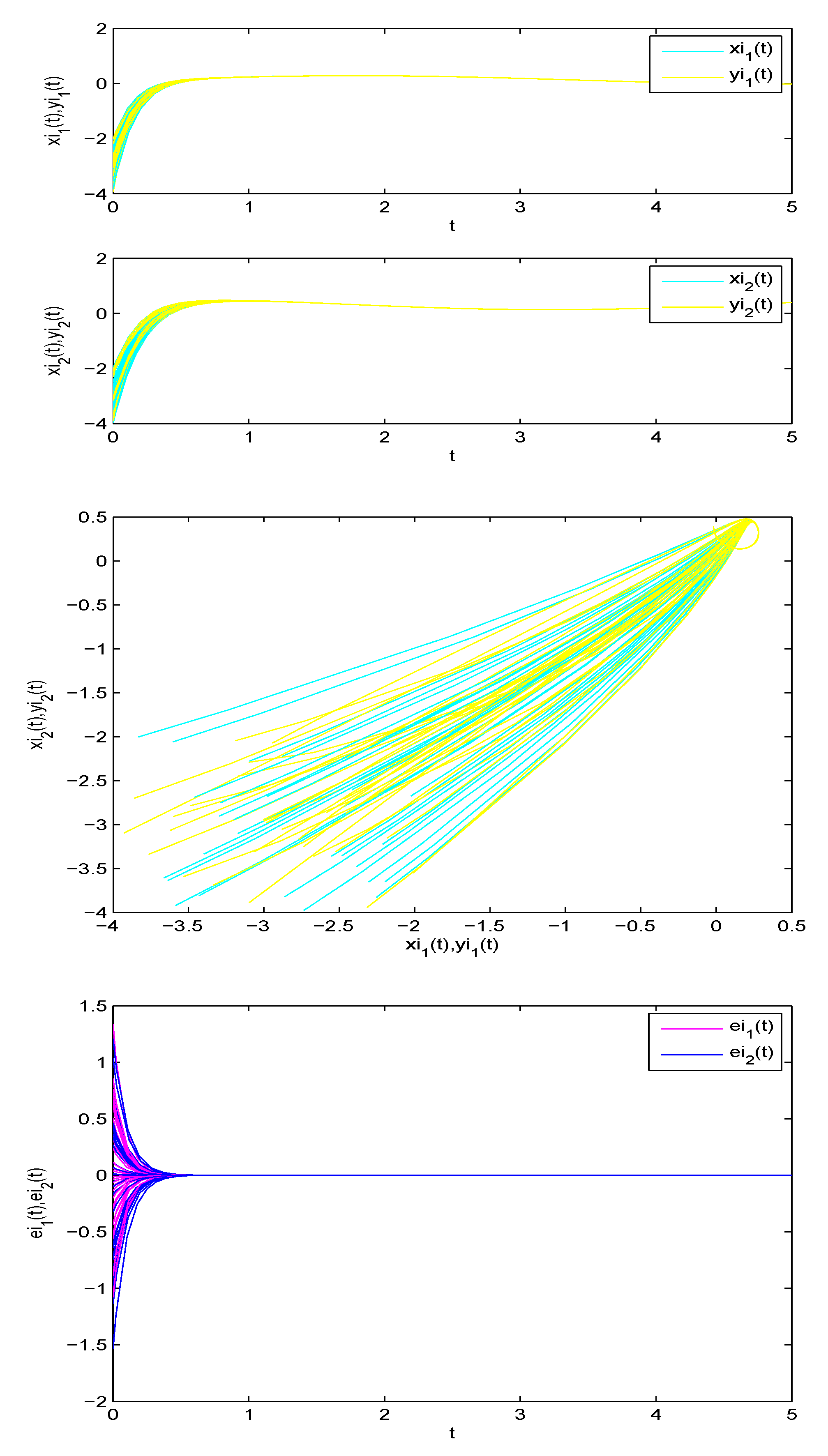
4. Numerical Simulation


| Condition | ||
|---|---|---|
| 1 | −16.37 | 2.4142 |
| 2 | −15.185 | 0.8321 |


| Condition | ||
|---|---|---|
| 1 | −6.525 | 3.9142 |
| 2 | −4.7814 | 1.1808 |
| Method | |
|---|---|
| [8] | 4.5 |
| condition 1 | 3.9142 |
| condition 2 | 1.1808 |

| Condition | ||
|---|---|---|
| 1 | −0.675 | 2.4142 |
| 2 | −1.675 | 0.8321 |
| Method | |
|---|---|
| [11] | 4.3784 |
| [45] | 4.3620 |
| [12] | 3.4259 |
| [13] | 2.3897 |
| condition 1 | 2.4142 |
| condition 2 | 0.8321 |


5. Conclusions
Author Contributions
Funding
Institutional Review Board Statement
Informed Consent Statement
Data Availability Statement
Conflicts of Interest
References
- Tyagi, S.; Martha, S.C. Finite-time stability for a class of fractional-order fuzzy neural networks with proportional delay. Fuzzy Sets Syst. 2020, 381, 68–77. [Google Scholar] [CrossRef]
- Xie, W.; Nguang, S.; Zhu, H.; Zhang, Y.; Shi, K. A novel event-triggered asynchronous H∞ control for T-S fuzzy Markov jump systems under hidden Markov switching topologies. Fuzzy Sets Syst. 2022, 443, 258–282. [Google Scholar] [CrossRef]
- Zhang, W.; Li, C.; Huang, T.; Huang, J. Fixed-time synchronization of complex networks with nonidentical nodes and stochastic noise perturbations. Phys. A 2018, 492, 1531–1542. [Google Scholar] [CrossRef]
- Chen, X.; Song, Q.; Li, Z.; Liu, Y. Stability analysis of continuous-time and discrete-time quaternion-valued neural networks with linear threshold neurons. IEEE Trans. Neural Netw. Learn. Syst. 2017, 29, 2769–2781. [Google Scholar] [CrossRef]
- Wei, R.; Cao, J. Fixed-time synchronization of quaternion-valued memristive neural networks with time delays. Neural Netw. 2019, 113, 1–10. [Google Scholar] [CrossRef]
- Zhang, R.; Zeng, D.; Park, J.H.; Lam, H.K.; Zhong, S. Fuzzy adaptive event-triggered sampled-data control for stabilization of T-S fuzzy memristive neural networks with reaction-diffusion terms. IEEE Trans. Fuzzy Syst. 2021, 29, 1775–1785. [Google Scholar] [CrossRef]
- Xiao, J.Y.; Li, Y.T.; Wen, S.P. Mittag-Leffler synchronization and stability analysis for neural networks in the fractional-order multi-dimension field. Knowl.-Based Syst. 2021, 231, 107404. [Google Scholar] [CrossRef]
- Ding, X.; Cao, J.; Alsaedi, A.; Alsaadi, F.E.; Hayat, T. Robust fixed-time synchronization for uncertain complex-valued neural networks with discontinuous activation functions. Neural Netw. 2017, 90, 42–55. [Google Scholar] [CrossRef]
- Hu, J.; Zeng, C.; Tan, J. Boundedness and periodicity for linear threshold discrete-time quaternion-valued neural network with time-delays. Neurocomputing 2017, 267, 417–425. [Google Scholar] [CrossRef]
- Li, H.; Li, C.; Huang, T.; Zhang, W. Fixed-time stabilization of impulsive Cohen-Grossberg BAM neural networks. Neural Netw. 2018, 98, 203–211. [Google Scholar] [CrossRef]
- Polyakov, A. Nonlinear feedback design for fixed-time stabilization of linear control systems. IEEE Trans. Autom. Control 2011, 57, 2106–2110. [Google Scholar] [CrossRef]
- Hu, C.; Yu, J.; Chen, Z.; Jiang, H.; Huang, T. Fixed-time stability of dynamical systems and fixed-time synchronization of coupled discontinuous neural networks. Neural Netw. 2017, 89, 74–83. [Google Scholar] [CrossRef]
- Chen, C.; Li, L.; Peng, H.; Yang, Y.; Zhao, H. A new fixed-time stability theorem and its application to the fixed-time synchronization of neural networks. Neural Netw. 2020, 123, 412–419. [Google Scholar] [CrossRef]
- Liu, H.; Wang, Z.; Shen, B.; Dong, H. Delay-Distribution-Dependent H∞ state estimation for discrete-time memristive neural networks with mixed time-delays and fading measurementss. IEEE Trans. Cybern. 2019, 50, 440–451. [Google Scholar] [CrossRef]
- Liu, H.; Wang, Z.; Shen, B.; Liu, X. Event-triggered H∞ state estimation for delayed stochastic memristive neural networks with missing measurements: The discrete-time case. IEEE Trans. Neural Netw. Learn. Syst. 2017, 29, 3727–3737. [Google Scholar]
- Zhang, R.; Zeng, D.; Park, J.H.; Lam, H.K.; Xie, X. Fuzzy sampled-data control for synchronization of T-S fuzzy reaction-diffusion neural networks with additive time-varying delays. IEEE Trans. Cybern. 2021, 51, 2384–2397. [Google Scholar] [CrossRef]
- Liu, X.; Ho, D.W.C.; Song, Q.; Xu, W. Finite/fixed-time pinning synchronization of complex networks with stochastic disturbances. IEEE Trans. Cybern. 2019, 49, 2398–2403. [Google Scholar]
- Liu, X.; Ho, D.W.C.; Xie, C. Prespecified-time cluster synchronization of complex networks via a smooth control approach. IEEE Trans. Cybern. 2020, 50, 1771–1775. [Google Scholar] [CrossRef]
- Liu, Y.; Zhang, D.; Lu, J.; Cao, J. Global μ-stability criteria for quaternion-valued neural networks with unbounded time-varying delays. Inf. Sci. 2016, 360, 273–288. [Google Scholar] [CrossRef]
- Liu, Y.; Zhang, D.; Lu, J. Global exponential stability for quaternion-valued recurrent neural networks with time-varying delays. Nonlinear Dyn. 2017, 87, 553–565. [Google Scholar] [CrossRef]
- Yang, X.; Li, C.; Song, Q.; Li, H.; Huang, J. Effects of state-dependent impulses on robust exponential stability of quaternion-valued neural networks under parametric uncertainty. IEEE Trans. Neural Netw. Learn. Syst. 2018, 30, 2197–2211. [Google Scholar] [CrossRef] [PubMed]
- Yang, X.; Li, C.; Song, Q.; Chen, J.; Huang, J. Global Mittag-Leffler stability and synchronization analysis of fractional-order quaternion-valued neural networks with linear threshold neurons. Neural Netw. 2018, 105, 88–103. [Google Scholar] [CrossRef] [PubMed]
- Xiao, J.Y.; Cao, J.D.; Cheng, J.; Zhong, S.M.; Wen, S.P. Novel methods to finite-time Mittag-Leffler synchronization problem of fractional-order quaternion-valued neural networks. Inf. Sci. 2020, 122, 320–327. [Google Scholar] [CrossRef]
- Xiao, J.Y.; Cao, J.D.; Cheng, J.; Wen, S.P.; Zhang, R.M.; Zhong, S.M. Novel inequalities to global Mittag-Leffler synchronization and stability analysis of fractional-order quaternion-valued neural networks. IEEE Trans. Neural Netw. Learn. Syst. 2021, 32, 3700–3709. [Google Scholar] [CrossRef]
- Xiao, J.Y.; Cheng, J.; Shi, K.B.; Zhang, R.M. A general approach to fixed-time synchronization problem for fractional-order multi-dimension-valued fuzzy neural networks based on memristor. IEEE Trans. Fuzzy Syst. 2021, 30, 968–977. [Google Scholar] [CrossRef]
- Xiao, J.Y.; Zhong, S.M.; Wen, S.P. Unified analysis on the global dissipativity and stability of fractional-order multidimension-valued memristive neural networks with time delay. IEEE Trans. Neural Netw. Learn. Syst. 2021. Online ahead of print. [Google Scholar] [CrossRef]
- Xiao, J.Y.; Zhong, S.M.; Wen, S.P. Improved approach to the problem of the global Mittag-Leffler synchronization for fractional-order multidimension-valued BAM neural networks based on new inequalities. Neural Netw. 2021, 133, 87–100. [Google Scholar] [CrossRef]
- Hardy, G.; Littlewood, J.; Poly, G. Inequalities; Cambridge University Press: Cambridge, UK, 1952. [Google Scholar]
- Ali, M.S.; Hymavathi, M.; Senan, S.; Shekher, V.; Arik, S. Global asymptotic synchronization of impulsive fractional-order complex-valued memristor-based neural networks with time varying delays. Commun. Nonlinear Sci. Numer. Simul. 2019, 78, 104869. [Google Scholar]
- Rajchakit, G.; Sriraman, R. Robust passivity and stability analysis of uncertain complex-valued impulsive neural networks with time-varying delays. Neural Processing Lett. 2021, 53, 581–606. [Google Scholar] [CrossRef]
- Rajchakit, G.; Chanthorn, P.; Niezabitowski, M.; Raja, R.; Baleanu, D.; Pratap, A. Impulsive effects on stability and passivity analysis of memristor-based fractional-order competitive neural networks. Neurocomputing 2020, 417, 290–301. [Google Scholar] [CrossRef]
- Li, H.; Kao, Y.; Li, H.L. Globally beta-Mittag-Leffler stability and beta-Mittag-Leffler convergence in Lagrange sense for impulsive fractional-order complex-valued neural networks. Chaos Solitons Fractals 2021, 148, 111061. [Google Scholar] [CrossRef]
- Yang, X.J.; Li, C.D.; Huang, T.W.; Song, Q.K.; Huang, J.J. Synchronization of fractional-order memristor-based complex-valued neural networks with uncertain parameters and time delays. Chaos Solitons Fractals 2018, 110, 105–123. [Google Scholar] [CrossRef]
- Aadhithiyan, S.; Raja, R.; Zhu, Q.; Alzabut, J.; Niezabitowski, M.; Lim, C.P. Modified projective synchronization of distributive fractional order complex dynamic networks with model uncertainty via adaptive control. Chaos Solitons Fractals 2021, 147, 110853. [Google Scholar] [CrossRef]
- Chanthorn, P.; Rajchakit, G.; Thipcha, J.; Emharuethai, C.; Sriraman, R.; Lim, C.P.; Ramachandran, R. Robust stability of complex-valued stochastic neural networks with time-varying delays and parameter uncertainties. Mathematics 2020, 8, 742. [Google Scholar] [CrossRef]
- Xiao, J.Y.; Guo, X.; Li, Y.T.; Wen, S.P.; Shi, K.B.; Tang, Y.Q. Extended Analysis on the global Mittag-Leffler synchronization problem for fractional-order octonion-valued BAM neural networks. Neural Netw. 2022, 154, 491–507. [Google Scholar] [CrossRef]
- Vadivel, R.; Hammachukiattikul, P.; Gunasekaran, N.; Saravanakumar, R.; Dutta, H. Strict dissipativity synchronization for delayed static neural networks: An event-triggered scheme. Chaos Solitons Fractals 2021, 150, 111212. [Google Scholar] [CrossRef]
- Arbi, A.; Cao, J.D.; Alsaedi, A. Improved synchronization analysis of competitive neural networks with time-varying delays. Nonlinear Anal. Model. Control 2018, 23, 82–107. [Google Scholar] [CrossRef]
- Arbi, A. Novel traveling waves solutions for nonlinear delayed dynamical neural networks with leakage term. Chaos Solitons Fractals 2021, 152, 111436. [Google Scholar] [CrossRef]
- Arbi, A.; Tahri, N.; Jammazi, C.; Huang, C.X.; Cao, J.D. Almost anti-periodic solution of inertial neural networks with leakage and time-varying delays on timescales. Circuits Syst. Signal Processing 2022, 41, 1940–1956. [Google Scholar] [CrossRef]
- Ali, M.S.; Hymavathi, M.; Rajchakit, G.; Saroha, S.; Palanisamy, L.; Hammachukiattikul, P. Synchronization of fractional order fuzzy BAM neural networks with time varying delays and reaction diffusion terms. IEEE Access 2020, 8, 186551–186571. [Google Scholar] [CrossRef]
- Anbuvithya, R.; Sri, S.D.; Vadivel, R.; Gunasekaran, N.; Hammachukiattikul, P. Extended dissipativity and non-fragile synchronization for recurrent neural networks with multiple time-varying delays via sampled-data control. IEEE Access 2021, 9, 31454–31466. [Google Scholar] [CrossRef]
- Vadivel, R.; Hammachukiattikul, P.; Rajchakit, G.; Ali, M.S.; Unyong, B. Finite-time event-triggered approach for recurrent neural networks with leakage term and its application. Math. Comput. Simul. 2021, 182, 765–790. [Google Scholar] [CrossRef]
- Xiao, J.Y.; Zhong, S.M. Synchronization and stability of delayed fractional-order memristive quaternion-valued neural networks with parameter uncertainties. Neurocomputing 2019, 363, 321–338. [Google Scholar] [CrossRef]
- Parsegov, S.; Polyakov, A.; Shcherbakov, P. Nonlinear fixed-time control protocol for uniform allocation of agents on a segment. Decis. Control 2013, 363, 321–338. [Google Scholar] [CrossRef]
Publisher’s Note: MDPI stays neutral with regard to jurisdictional claims in published maps and institutional affiliations. |
© 2022 by the authors. Licensee MDPI, Basel, Switzerland. This article is an open access article distributed under the terms and conditions of the Creative Commons Attribution (CC BY) license (https://creativecommons.org/licenses/by/4.0/).
Share and Cite
Xiao, J.; Li, Y. Novel Synchronization Conditions for the Unified System of Multi-Dimension-Valued Neural Networks. Mathematics 2022, 10, 3031. https://doi.org/10.3390/math10173031
Xiao J, Li Y. Novel Synchronization Conditions for the Unified System of Multi-Dimension-Valued Neural Networks. Mathematics. 2022; 10(17):3031. https://doi.org/10.3390/math10173031
Chicago/Turabian StyleXiao, Jianying, and Yongtao Li. 2022. "Novel Synchronization Conditions for the Unified System of Multi-Dimension-Valued Neural Networks" Mathematics 10, no. 17: 3031. https://doi.org/10.3390/math10173031