


Breast Abnormality Boundary Extraction in Mammography Image Using Variational Level Set and Self-Organizing Map (SOM)

 , , and
Abstract
: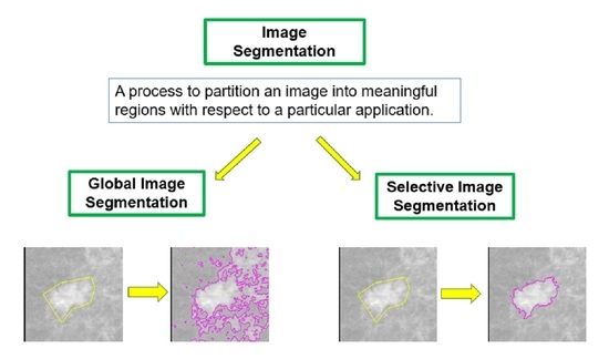
1. Introduction
2. Review of the Existing Models
2.1. Chan and Vese (CV) Model
2.2. SOM-Based Chan–Vese (SOMCV) Model
2.3. Primal-Dual Selective Segmentation 2 (PD2) Model
3. The Proposed Models
3.1. Derivation of Euler Lagrange (EL) Equation
3.2. A New Variant of the SSOM Model
3.3. Steps of the Algorithm for the Proposed SSOM and SSOMH Models
| Algorithm 1: Algorithm for the SSOM Model. |
|
| Algorithm 2: Algorithm for SSOMH Model. |
|
3.4. Convergence Analysis
- is a closed mapping;
- is continuous;
- is closed at ;
- is a decent function of and ;
- The sequence is contained in a compact set, .
4. Experimental Results
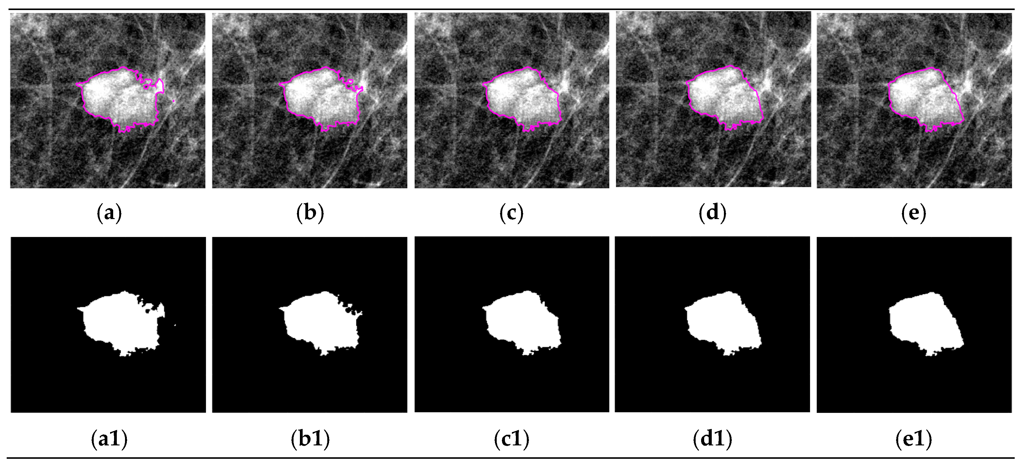
4.1. Segmentation Results of Test Images from the INbreast Database
4.2. Segmentation Results of Test Images from the CBIS-DDSM Database
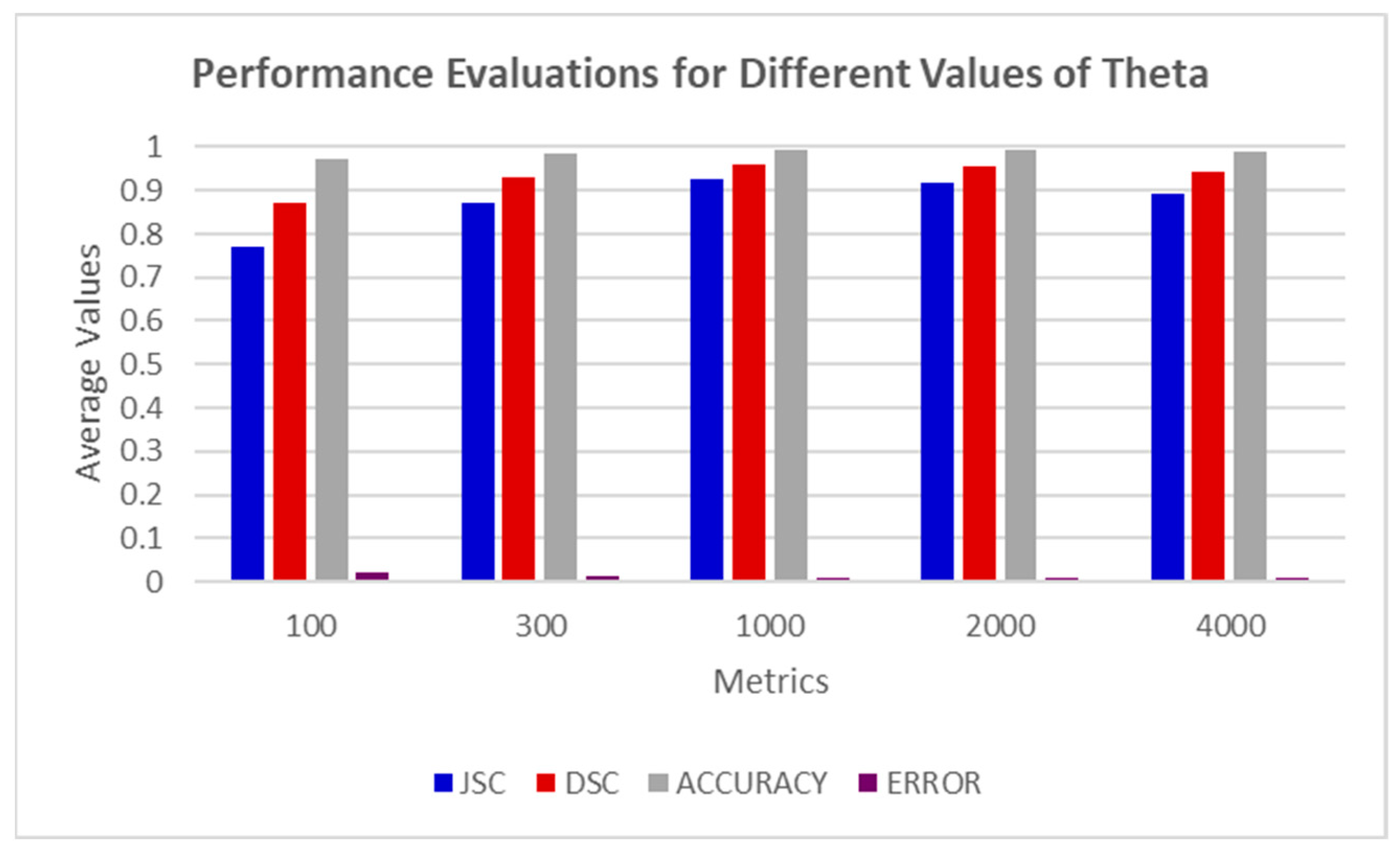
4.3. Results of SSOMH Model with Different Values of Area Parameter θ
5. Conclusions
Author Contributions
Funding
Data Availability Statement
Conflicts of Interest
References
- Ministry of Health. Malaysia National Cancer Registry 2012–2016; Ministry of Health: Putrajaya, Malaysia, 2019. Available online: https://drive.google.com/file/d/1BuPWrb05N2Jez6sEP8VM5r6JtJtlPN5W/view (accessed on 1 November 2021).
- Spreafico, F.S.; Cardoso-filho, C.; Cabello, C.; Sarian, L.O.; Zeferino, L.C.; Vale, D.B. Breast Cancer in Men: Clinical and Pathological Analysis of 817 Cases. Am. J. Men’s Health 2020, 14, 1–6. [Google Scholar] [CrossRef] [PubMed]
- Shamsi, M.; Islamian, J.P. Breast cancer: Early diagnosis and effective treatment by drug delivery tracing. Nucl. Med. Rev. 2017, 20, 45–48. [Google Scholar] [CrossRef]
- Yasiran, S.S.; Jumaat, A.K.; Manaf, M.; Ibrahim, A.; Wan Eny Zarina, W.A.R.; Malek, A.; Laham, M.F.; Mahmud, R. Comparison between GVF Snake and ED Snake in Segmenting Microcalcifications. In Proceedings of the 2011 IEEE International Conference on Computer Applications and Industrial Electronics (ICCAIE), Penang, Malaysia, 4–7 December 2011; pp. 597–601. [Google Scholar]
- Chen, K. Introduction to variational image-processing models and applications. Int. J. Comput. Math. 2013, 90, 1–8. [Google Scholar] [CrossRef]
- Rick, A.; Bothorel, S.; Bouchon-Meunier, B.; Muller, S.; Rifqi, M. Fuzzy techniques in mammographic image processing. In Fuzzy Techniques in Image Processing; Physica: Heidelberg, Germany, 2000; pp. 308–336. [Google Scholar]
- Yearwood, A.B. A Brief Survey on Variational Methods for Image Segmentation. 2010, pp. 1–7. Available online: researchgate.net/profile/Abdu-Badru-Yearwood/publication/323971382_A_Brief_Survey_on_Variational_Methods_for_Image_Segmentation/links/5abd38e8a6fdcccda6581b05/A-Brief-Survey-on-Variational-Methods-for-Image-Segmentation.pdf (accessed on 1 November 2021).
- Vlachos, I.K.; Sergiadis, G.D. Intuitionistic Fuzzy Image Processing. In Soft Computing in Image Processing; Springer: Berlin/Heidelberg, Germany, 2007; pp. 383–414. [Google Scholar]
- Chowdhary, C.L.; Acharjya, D.P. Segmentation of mammograms using a novel intuitionistic possibilistic fuzzy c-mean clustering algorithm. In Nature Inspired Computing; Advances in Intelligent Systems and Computing; Springer: Singapore, 2018; pp. 75–82. [Google Scholar] [CrossRef]
- Ghosh, S.K.; Mitra, A.; Ghosh, A. A novel intuitionistic fuzzy soft set entrenched mammogram segmentation under Multigranulation approximation for breast cancer detection in early stages. Expert Syst. Appl. 2021, 169, 114329. [Google Scholar] [CrossRef]
- Chowdhary, C.L.; Mittal, M.; P., K.; Pattanaik, P.A.; Marszalek, Z. An efficient segmentation and classification system in medical images using intuitionist possibilistic fuzzy C-mean clustering and fuzzy SVM algorithm. Sensors 2020, 20, 3903. [Google Scholar] [CrossRef] [PubMed]
- Chaira, T. An Intuitionistic Fuzzy Clustering Approach for Detection of Abnormal Regions in Mammogram Images. J. Digit. Imaging 2021, 34, 428–439. [Google Scholar] [CrossRef]
- Atiqah, N.; Zaman, K.; Eny, W.; Wan, Z.; Rahman, A.; Jumaat, A.K.; Yasiran, S.S. Classification of Breast Abnormalities Using Artificial Neural Network. AIP Conf. Proc. 2015, 1660, 050038. [Google Scholar] [CrossRef]
- Ronneberger, O.; Fischer, P.; Brox, T. U-net: Convolutional networks for biomedical image segmentation. In Proceedings of the International Conference on Medical Image Computing and Computer-Assisted Intervention: 2015 18th International Conference, Munich, Germany, 5–9 October 2015; Part III. pp. 234–241. [Google Scholar]
- Michael, E.; Ma, H.; Li, H.; Kulwa, F.; Li, J. Breast Cancer Segmentation Methods Current Status and Future Potentials. Biomed Res. Int. 2021, 2021, 9962109. [Google Scholar] [CrossRef] [PubMed]
- Saravanan, R.; Sujatha, P. A State of Art Techniques on Machine Learning Algorithms: A Perspective of Supervised Learning Approaches in Data Classification. In Proceedings of the 2018 Second International Conference on Intelligent Computing and Control Systems (ICICCS), Madurai, India, 14–15 June 2018; pp. 945–949. [Google Scholar]
- Barbu, T.; Marinoschi, G.; Moroanu, C.; Munteanu, I. Advances in Variational and Partial Differential Equation-Based Models for Image Processing and Computer Vision. Math. Probl. Eng. 2018, 2018, 1701052. [Google Scholar] [CrossRef]
- Jumaat, A.K.; Chen, K. A Reformulated Convex and Selective Variational Image Segmentation Model and its Fast Multilevel Algorithm. Numer. Math. Theory Methods Appl. 2019, 12, 403–437. [Google Scholar]
- Rahmati, P.; Adler, A.; Hamarneh, G. Mammography segmentation with maximum likelihood active contours. Med. Image Anal. 2012, 16, 1167–1186. [Google Scholar] [CrossRef] [PubMed]
- Ciecholewski, M. Malignant and benign mass segmentation in mammograms using active contour methods. Symmetry 2017, 9, 277. [Google Scholar] [CrossRef]
- Chan, T.F.; Vese, L.A. Active contours without edges. IEEE Trans. Image Process. 2001, 10, 266–277. [Google Scholar] [CrossRef] [PubMed]
- Saraswathi, D.; Srinivasan, E.; Ranjitha, P. An Efficient Level Set Mammographic Image Segmentation using Fuzzy C Means Clustering. Asian J. Appl. Sci. Technol. 2017, 1, 7–11. [Google Scholar]
- Somroo, S.; Choi, K.N. Robust active contours for mammogram image segmentation. In Proceedings of the 2017 IEEE International Conference on Image Processing (ICIP), Beijing, China, 17–20 September 2017; pp. 2149–2153. [Google Scholar]
- Hmida, M.; Hamrouni, K.; Solaiman, B.; Boussetta, S. Mammographic mass segmentation using fuzzy contours. Comput. Methods Programs Biomed. 2018, 164, 131–142. [Google Scholar] [CrossRef]
- Radhi, E.A.; Kamil, M.Y. Segmentation of breast mammogram images using level set method. AIP Conf. Proc. 2022, 2398, 020071. [Google Scholar]
- Badshah, N.; Atta, H.; Ali Shah, S.I.; Attaullah, S.; Minallah, N.; Ullah, M. New local region based model for the segmentation of medical images. IEEE Access 2020, 8, 175035–175053. [Google Scholar] [CrossRef]
- Jumaat, A.K.; Chen, K.E. An optimization-based multilevel algorithm for variational image segmentation models. Electron. Trans. Numer. Anal. 2017, 46, 474–504. [Google Scholar]
- Jumaat, A.K.; Chen, K. Three-Dimensional Convex and Selective Variational Image Segmentation Model. Malays. J. Math. Sci. 2020, 14, 81–92. [Google Scholar]
- Jumaat, A.K.; Chen, K. A fast multilevel method for selective segmentation model of 3-D digital images. Adv. Stud. Math. J. 2022, 127–152. Available online: https://tcms.org.ge/Journals/ASETMJ/Special%20issue/10/PDF/asetmj_SpIssue_10_9.pdf (accessed on 1 November 2021).
- Acho, S.N.; Rae, W.I.D. Interactive breast mass segmentation using a convex active contour model with optimal threshold values. Phys. Med. 2016, 32, 1352–1359. [Google Scholar] [CrossRef]
- Ali, H.; Faisal, S.; Chen, K.; Rada, L. Image-selective segmentation model for multi-regions within the object of interest with application to medical disease. Vis. Comput. 2020, 37, 939–955. [Google Scholar] [CrossRef]
- Ghani, N.A.S.M.; Jumaat, A.K. Selective Segmentation Model for Vector-Valued Images. J. Inf. Commun. Technol. 2022, 5, 149–173. Available online: http://e-journal.uum.edu.my/index.php/jict/article/view/8062 (accessed on 1 November 2021).
- Nguyen, T.N.A.; Cai, J.; Zhang, J.; Zheng, J. Robust Interactive Image Segmentation Using Convex Active Contours. IEEE Trans. Image Process. 2012, 21, 3734–3743. [Google Scholar] [CrossRef] [PubMed]
- Ghani, N.A.S.M.; Jumaat, A.K.; Mahmud, R. Boundary Extraction of Abnormality Region in Breast Mammography Image using Active Contours. ESTEEM Acad. J. 2022, 18, 115–127. [Google Scholar]
- Zhang, K.; Song, H.; Zhang, L. Active contours driven by local image fitting energy. Pattern Recognit. 2010, 43, 1199–1206. [Google Scholar] [CrossRef]
- Abdelsamea, M.M.; Gnecco, G.; Gaber, M.M. A SOM-based Chan-Vese model for unsupervised image segmentation. Soft Comput. 2017, 21, 2047–2067. [Google Scholar] [CrossRef]
- Mumford, D.; Shah, J. Optimal approximations by piecewise smooth functions and associated variational problems. Commun. Pure Appl. Math. 1989, 42, 577–685. [Google Scholar] [CrossRef]
- Osher, S.; Sethian, J.A. Fronts propagating with curvature-dependent speed: Algorithms based on Hamilton-Jacobi formulations. J. Comput. Phys. 1988, 79, 12–49. [Google Scholar] [CrossRef]
- Altarawneh, N.M.; Luo, S.; Regan, B.; Sun, C.; Jia, F. Global Threshold and Region-Based Active Contour Model For Accurate Image Segmentation. Signal Image Process. 2014, 5, 1–11. [Google Scholar] [CrossRef]
- Chen, B.L. Optimization Theory and Algorithms, 2nd ed.; Tsinghua University Press: Beijing, China, 1989. [Google Scholar]
- Moreira, I.C.; Amaral, I.; Domingues, I.; Cardoso, A.; Cardoso, M.J.; Cardoso, J.S. INbreast: Toward a Full-field Digital Mammographic Database. Acad. Radiol. 2012, 19, 236–248. [Google Scholar] [CrossRef] [PubMed]
- Lee, R.S.; Gimenez, F.; Hoogi, A.; Miyake, K.K.; Gorovoy, M.; Rubin, D.L. Data Descriptor: A curated mammography data set for use in computer-aided detection and diagnosis research. Sci. Data 2017, 4, 170177. [Google Scholar] [CrossRef] [PubMed]
- Azam, A.S.B.; Malek, A.A.; Ramlee, A.S.; Suhaimi, N.D.S.M.; Mohamed, N. Segmentation of Breast Microcalcification Using Hybrid Method of Canny Algorithm with Otsu Thresholding and 2D Wavelet Transform. In Proceedings of the 2020 10th IEEE International Conference on Control System, Computing and Engineering (ICCSCE), Penang, Malaysia, 21–22 August 2020; pp. 91–96. [Google Scholar] [CrossRef]


| Model | JSC | DSC | Accuracy | Error |
|---|---|---|---|---|
| SOMCV | 0.434 | 0.584 | 0.735 | 0.265 |
| IIS | 0.801 | 0.887 | 0.961 | 0.040 |
| U-NET | 0.519 | 0.674 | 0.847 | 0.153 |
| PD2 | 0.819 | 0.899 | 0.962 | 0.038 |
| SSOM | 0.883 | 0.937 | 0.976 | 0.024 |
| SSOMH | 0.884 | 0.938 | 0.977 | 0.023 |
| Model | Computation Time (Seconds) | |
|---|---|---|
| Training | Testing | |
| SOMCV | 0.05 | 1.67 |
| U-NET | 327.00 | 0.76 |
| PD2 | Not Related | 71.03 |
| SSOM | 0.05 | 1.42 |
| SSOMH | 0.05 | 1.39 |
| Model | JSC | DSC | Accuracy | Error |
|---|---|---|---|---|
| SOMCV | 0.425 | 0.576 | 0.695 | 0.304 |
| IIS | 0.449 | 0.616 | 0.778 | 0.222 |
| U-NET | 0.569 | 0.712 | 0.893 | 0.107 |
| PD2 | 0.768 | 0.867 | 0.945 | 0.055 |
| SSOMH | 0.856 | 0.920 | 0.964 | 0.036 |
| Model | Computation Time (Seconds) | |
|---|---|---|
| Training | Testing | |
| SOMCV | 0.05 | 1.79 |
| U-NET | 307.00 | 0.73 |
| PD2 | Not Related | 98.54 |
| SSOMH | 0.05 | 0.8 |
Disclaimer/Publisher’s Note: The statements, opinions and data contained in all publications are solely those of the individual author(s) and contributor(s) and not of MDPI and/or the editor(s). MDPI and/or the editor(s) disclaim responsibility for any injury to people or property resulting from any ideas, methods, instructions or products referred to in the content. |
© 2023 by the authors. Licensee MDPI, Basel, Switzerland. This article is an open access article distributed under the terms and conditions of the Creative Commons Attribution (CC BY) license (https://creativecommons.org/licenses/by/4.0/).
Share and Cite
Ghani, N.A.S.M.; Jumaat, A.K.; Mahmud, R.; Maasar, M.A.; Zulkifle, F.A.; Jasin, A.M. Breast Abnormality Boundary Extraction in Mammography Image Using Variational Level Set and Self-Organizing Map (SOM). Mathematics 2023, 11, 976. https://doi.org/10.3390/math11040976
Ghani NASM, Jumaat AK, Mahmud R, Maasar MA, Zulkifle FA, Jasin AM. Breast Abnormality Boundary Extraction in Mammography Image Using Variational Level Set and Self-Organizing Map (SOM). Mathematics. 2023; 11(4):976. https://doi.org/10.3390/math11040976
Chicago/Turabian StyleGhani, Noor Ain Syazwani Mohd, Abdul Kadir Jumaat, Rozi Mahmud, Mohd Azdi Maasar, Farizuwana Akma Zulkifle, and Aisyah Mat Jasin. 2023. "Breast Abnormality Boundary Extraction in Mammography Image Using Variational Level Set and Self-Organizing Map (SOM)" Mathematics 11, no. 4: 976. https://doi.org/10.3390/math11040976