1. Introduction
A control system is a tool that directs and regulates the behavior of a device or process to the desired values by generating and executing a set of control commands and inputs. One of the new control methods that have a clear and active system model in the controller structure is the model predictive control (MPC) method [
1,
2,
3,
4,
5]. Predictive control refers to a set of algorithms that calculate the control signal to optimize the future behavior of a system. This method has been developed since the 1970s and has been widely used in industrial processes. However, most MPC techniques are focused on discrete time and less so on continuous time. Various methods and techniques have been developed in recent years to solve the problem of continuous-time prediction control, which can be mentioned as follows [
6,
7,
8,
9,
10].
In [
11], based on the direct multiple throwing methods, the forecast horizon is divided into subintervals, and by discretizing the control variables and parameterizing the state variables, the optimal control problem with infinite dimension to the nonlinear programming problem. After completing these steps, the NLP problem is solved using fast numerical methods based on the derived information. In [
12], in each sampling interval, the control variable is considered a constant function. The main feature of the proposed method is the fragmentary nature of the control signal. This feature leads to a solvable optimization problem in which the number of control variables is reduced. In [
13], to reduce the computational volume and speed up the optimization process, by considering a set of orthogonal real functions, the control function is expressed as a series of them. The article [
14], first turns the problem of optimal control into a problem of nonlinear programming with the method of orthogonal accompaniment. Then, to find the absolute minimum of the optimization problem, it uses global optimization methods. In [
15], using the direct method, the continuous-time predictor control problem and the optimal control problem are converted into NLP problems at any time of sampling, i.e., by parameterization and discretization of control and state variables, and it is then solved using the nonlinear programming method.
Moreover, in [
16], the authors addressed the issue that the discretization of the optimal control problem in MPC is often performed at points of equal distance, and only if the sampling intervals are small enough, and if this discretization has the necessary accuracy. For this purpose, to improve the discretization accuracy and prevent the use of a large number of subsets, a quasi-spectral method has been used that approximates the state and control variables with Lagrange polynomials. In [
17], the problem of tracking for nonlinear systems using MPC is stated. In this way, by first obtaining successive derivations of the system output equation and using them in the Taylor expansion of the system output, the tracking error in the predictor horizon is approximated by the Taylor series expansion. Then, the present optimization problem is solved using conventional methods. In [
18], the authors proposed a design of model predictive control for discrete-time nonlinear systems using global optimization. Since the problem of nonlinear programming may be nonconvex, if it was first convex, it is treated using existing methods and then solved after linearization. In 2010, the authors proposed a solution to the continuous-time linear regulator problem. First, the period was subdivided into sub-bases by appropriate methods, and in each subperiod, the control function was parameterized into one of three methods: zero-order maintenance, partial linear maintenance, and one-order maintenance. Then, by converting the optimal control problem into the form of a finite-dimensional optimization problem, they determined the unknown parameters in the parameterizations. In this way, the optimal control variables are determined [
19]. The problem of nonlinear prediction control using a free derivative optimization algorithm is proposed in [
20]. Since optimization methods are based on gradients, they are not suitable for functions that are not derivative. Therefore, the free derivative algorithm was investigated and used in this paper. Of course, first, the optimal control problems in predictive control were parameterized using the throwing method, and, then, the resulting nonlinear programming problem was solved using a free derivative algorithm. There are also many other challenges in the field of control. For example, regarding trajectory tracking, various research studies have been carried out in [
21,
22,
23,
24,
25,
26], which can be interesting for those interested. On the other hand, with progress in various control fields, new methods were also proposed to solve existing challenges [
27,
28,
29,
30]. Among these challenges, we can mention the efficiency of robot transmission. In many studies, methods have been proposed to increase the transfer efficiency of robots. Among the proposed methods, we can mention event-triggered control [
31,
32,
33,
34,
35,
36].
According to the studies, in all of the above methods, while solving the problem of continuous-time predictor control, linearization, discretization, or parameterization methods have been used, and none of them has solved the problem of continuous-time predictor control. On the other hand, as we know, the issue of robust control in continuous-time space is rich. Therefore, these are the motivations of this paper, to propose continuous-time prediction control, and it is shown that the design of continuous-time nonlinear predictive controller design is equivalent to a system of differential-algebraic equations. Then, by solving this device using the semianalytical method of the homotopy perturbation method, the control function and the optimal state function are determined continuously.
The general structure of the sections of this article is such that first, the problem is studied in this research, i.e., the problem of continuous-time predictor control is stated in the second part. Since, at each moment of updating the algorithm, an optimal control problem must be solved, so in the third section, the optimal control problem and its solution approaches are repeated. On the other hand, to solve the problem of optimal control, an indirect method has been used, As a result, differential-algebraic equations with boundary conditions are created. To solve this device, the semianalytical method of homotopy perturbation has been used, which is mentioned in the fourth section. In the fifth section, the proposed design algorithm for predicting continuous-time systems is presented. In the sixth section, numerical examples and simulations, and in the seventh section, the conclusion is presented.
2. Problem Statement of Continuous-Time Predictive Control
Consider the following nonlinear continuous-time system:
With the state
, the initial condition is
, the output is
, and the control input is
, where
U is a compact set containing the origin. The nonlinear function
and
are smooth (continuous and derivative) with respect to all components. Here, it is assumed that system (1) has a unique solution for each initial condition
∈
nd for each continuous control function
[
37,
38,
39,
40].
According to the designer’s goal, which is usually to bring the state or output of the system to the desired value with minimal control effort, a cost function with the following infinite horizon is considered:
where
is a continuous function. Thus, problems (1) and (2) form an optimization problem with differential-algebraic constraints. If this optimization problem can be solved for the infinite horizon and there is also no model or system mismatch, then the control function found at the moment
t = 0 can be applied to the system at all times that
t ≥ 0. This is not the case in general, and because of confusion and model-system mismatch, the actual system behavior is different from the predicted behavior of the model. In this paper, to compensate for this difference, slide horizon control techniques such as predictive control can be used.
In predictive control, first, based on the current conditions of state variables, predicting the future behavior of the system from the system model and considering the cost function, the optimal controls are calculated. Then, the calculated optimal controls are applied to the dynamic system in a small part of the time interval. By moving the sampling interval forward and repeating this process, a control loop is created. This closed control loop is obtained by calculating the optimal controls of the instantaneous conditions of the state variables. According to the idea of predictive control and the theory of optimal control, it can be said that the design of the predictive controller for continuous-time systems (1) and (2) is performed according to the following Algorithm 1 in four steps:
| Algorithm 1: Predictive controller for continuous-time systems (1) and (2) |
| 0. The HP prediction horizon, update step, δ > 0 (note that δ is not necessarily a constant value but is smaller than the prediction horizon), and consider the sequence of update moments , such that . |
| 1. Measure or determine the state of the system at the , moment. |
| 2. Define the optimal control problem below, and solve it to determine the answer of |
| x( |
| where represents the set of all continuous functions of the segment . |
| 3. Apply control on the system in the range and ignore the remaining control signal. |
| 4. Repeat the above process for the next update moment . |
In the next sections, we will study and examine the equations as well as their control structures. For further information on these equations, you can refer to references [
41,
42,
43,
44,
45].
3. Optimal Control Problem and Approaches to Solve It
As stated in
Section 2, in each step of predictive control, we encounter an OC problem that can be expressed as follows:
The purpose of solving the optimal control problem is to determine the acceptable control function
, which causes the system to follow the acceptable state function
and minimize the
function. To solve this problem and ensure the stability of the steady state, the fin function
, which is a function of the finite time and the final state, is added to the cost function, and, thus, the cost function
is changed as follows:
Definition 1. A pair of is an acceptable answer for (3) if it holds true in the constraints of the problem.
Definition 2. The acceptable answer is the weak local minimum of the problem (3) with the cost function (4) if it is said that if we have for , > 0 and for all acceptable answers for that apply to conditions and . The local minimum is usually called the optimal answer.
Definition 3. The answer of is called the absolute minimum if the above conditions are met for , = ∞.
In general, there are three common methods to solve the problem of optimal control: the dynamic programming method, the direct method, and the indirect method. In the dynamic programming method [
11], an optimization policy is obtained by applying the “optimization principle”, which leads to solving sequential equations. In direct methods [
12], through the discretization and parameterization of variables, the optimal control problem becomes a nonlinear programming problem. Then, the resulting problem is solved using conventional algorithms. In the indirect methods, using the changing calculus and the Pontryagin minimum principle, the necessary optimal conditions, which constitute a two-point boundary value problem, are extracted. Then, by solving it with the relevant methods, the control function and the optimal state function are obtained. In this paper, the indirect method is utilized to solve the optimal control problem. The following is an indirect case study.
Indirect Method of Solving Optimal Control Problems
In the indirect method of solving the optimal control problem, due to the benefit of the analytical process and the issues of change calculation, the obtained answer is valid at least in the necessary conditions. Therefore, it seems that this method can provide the optimal answer with high accuracy among the optimal control problem-solving methods [
46,
47,
48].
Theorem 1. Assume that is the local minimum of the problem (3) with the cost function (4). Then, the function also has a derivative continuous state , such that, according to the Hamiltonian function:
The following relationships are established:
and
Equation emphasizes the “Pontryagin minimization principle”, where must minimize the Hamiltonian
Theorem 2. Suppose that
is an acceptable answer to the problem (3) with a cost function (4) that holds in the necessary conditions of optimality. If is a derivative and convex of any of the components with respect to for any , then (x(t),u(t)) is an absolute minimum of the optimal control problem.
According to the hypotheses of the above theorems, by solving the device (6), we can find the optimal solution to the optimal control problem (3) with the cost function (4). The set of equations (6) is a boundary value problem, such that if the differential equations and algebraic equations are nonlinear and its initial and boundary conditions are linear, it is difficult to find an accurate and analytical solution. In [
14], the semianalytical method of homotopy perturbation is used to solve it.
4. Homotopy Perturbation Method
Most of the phenomena we encounter in nature and technology are modeled using nonlinear differential equations, which, in many cases, it is not possible to find the exact answer. There are various semianalytical and numerical methods for solving nonlinear differential equations. The semianalytical method of homotopy perturbation is used to solve nonlinear equations [
15] of the system of differential-algebraic equations with initial values [
16], partial differential equations [
17], etc.
The hematopoietic disorder method is a combination of the classical disorder method and the homotopy method [
48]. The perturbation method is based on the existence of a parameter or small variables (perturbation) in the equation. To improve this method and apply it to unbalanced equations, some solutions have been proposed [
49,
50]. In this way, first, using the concept of homotopy in topology, an attempt has been made to construct a homotopic equation relating to the desired equation. In this homotopic equation, there is a perturbation parameter that changes in the range [1 and 0]. Then, the disorder method was applied to the homotopic equation. In the perturbation method, first, the solution of the equation is considered as a series of powers according to the perturbation parameter with unknown coefficients (function). Then, by substituting that series in the homotopic equation and equating the same power coefficients of the perturbation parameter, linear equations are obtained, which, by solving them sequentially, unknown functions in the series are obtained. To explain the main idea of the homotopy perturbation methodology, the following differential equation is considered:
where
is a general differential operator,
is a boundary operator, and
f(
t) is a known analytical function. In general, operator
can be divided into
and
, where
and
are linear and nonlinear operators, respectively. Thus, Equation (8) can be formulated as:
To solve Equation (9), first, the
homotopic is constructed that holds in the following condition:
where
is an unknown function,
is a substitution parameter, and
is an initial approximation of the solution of the differential Equation (8) that must hold in the boundary condition. It is clear from Equation (10) that when
p = 0, it is
, and when
p = 1, it is
. In other words, by changing
p from zero to one, the answer of
changes uniformly from
to
. Suppose the answer to Equation (9) is written as a series of
:
where
are unknown functions that are obtained according to the perturbation method. By placing
p = 1 in (10), the approximate answer to Equation (8) is obtained:
The convergence rate of the series (11) depends on the actual solution of Equation (7) for the A(
) operator. By substituting Equation (10) for homotopy (9) and equating the same power coefficients p on both sides of the equation, the following equations are obtained:
where
are the coefficients
in the nonlinear operator
ℵ:
where
are easily obtained by solving Equation (13).
5. The Proposed Method
As stated in
Section 2, according to Algorithm 1, the continuous-time prediction control problem is performed repeatedly in four steps. Now, considering the system dynamics, cost function, and indirect method of solving the optimal control problem, we can present the following algorithm to solve the continuous-time prediction control problem. Consider the following cost function and dynamic system:
The design of the predictive controller for the problem (14), which is a feedback controller in the framework of sliding horizon control, is carried out by solving the system of differential-algebraic equations according to the following Algorithm 2 in four steps:
| Algorithm 2: Predictive controller for the problem (14) |
| 0. The HP forecast horizon, the update step , (note that δ is not necessarily a fixed value but is defined as smaller than the forecast horizon), and the sequence of update moments , such as . |
| 1. Solve the system of differential-algebraic equations of the following DAEs using the method of homotopy perturbation to obtain approximate answers of state functions, both state and control, in the range of |
| 2. Apply control over the system in the range of and ignore the rest of the control signal. |
| 3. Determine the system state at moment with the state function obtained in step (1), . |
| 4. Repeat the above process for the next update moment . |
To perform the first step of the above algorithm, we go through the following steps:
In the hematopoietic disorder method, first, a homotopy is made corresponding to each of the equations (algebraic and differential) of the device (15). Approximate answers for the device (15) are considered a series of arbitrary order s, with unknown coefficients, such as the following, which, by substituting them in the constructed homotopies, the unknown functions of the series are obtained:
Then, by setting
p = 1, the approximate answers of the device (15) are determined:
To solve the device (15) by the method of homotopy perturbation, the initial values of the state variables, , are not known. Therefore, α ∈ are first considered unknowns. Then, after solving the device, unknown values of α are obtained according to the boundary condition.
Note 1. To implement the designed time controller, we implement it as a data sample so that the effect of discretization can be seen in the implementation of the designed continuous controller in digital systems.
Stability
In MPC, an optimal infinite horizon control problem is approximated by a sequence of finite horizon problems in the context of a slippery horizon control. In general, the stability of the closed-loop system is not guaranteed due to the use of finite predictive horizons. To achieve sustainability, various methods and techniques have been proposed. In [
44], considering hypotheses on system dynamics, the sentence adds the finite
condition to the cost function and the final unequal constraint
to the constraints of the optimal open-loop control problem. Then, the existence and method of selecting the fine matrix show the final state P and the final region Ω in such a way that the condition of the stability of the closed-loop system is guaranteed. Of course, the stated conditions are sufficient for sustainability and are not necessary. The presence of an added final inequality constraint makes it difficult to solve the optimal open-loop control problem, and the online execution of the problem is difficult in terms of computational time.
In [
49], it is shown that a suitable choice for the forecasting horizon can ensure the establishment of the final inequality constraint Lemma 2, as described in [
39]. Then, in Theorem 1, in [
38], the stability conditions of the closed-loop system are stated. In [
45], the stability analysis of sliding horizon controllers based on the Lyapunov function as the final penalty term was investigated. Theorem 4 in [
20] states the existence of a forecast horizon that guarantees the stability of the closed-loop system.
6. Simulation
In this section, to show the capability and efficiency of the proposed algorithm, the performance of the proposed method for designing a predictive controller for a CE150 laboratory helicopter is reviewed. In a helicopter, the angles of the main and lateral rotation planes are fixed, and the only function of the blades is to maintain angular balance in both vertical and horizontal planes with angular characteristics and . The only control inputs of the helicopter are the number of revolutions of its blades, which are denoted by u1 and u2. The torque produced by the main blade mainly affects the vertical plane Elevation (), and the torque produced by the side blade affects the horizontal plane Azimuth (). By examining the controllability and visibility conditions of the two horizontal and vertical SISO subsystems, we make sure that both are controllable.
In this section, the goal is to control the separate SISO path horizontally. In practice, two independent SISO subsystems can be created by tightening each of the two separate screws embedded in the horizontal and vertical planes to prevent the helicopter from moving and by not commanding the locked path entrance. To begin the design of the controller, we first consider the nonlinear differential equations of the helicopter governing state space:
In the stated dynamic model, four state variables express the state and behavior of the system at any given time, and there is a control variable that controls how the system behaves. The parameters of this model are given in
Table 1, where
is the rotor thrust and
is the moment of inertia for which the moments of inertia terms can be found using the definition assuming that the point mass weight is concentrated at the motors and the counterweight. Further, the rest of the parameters are constant coefficients.
Since the cost function is written based on state variables, the following equations must be solved to obtain the equilibrium
point, assuming the reference
output, and the state in which the helicopter is directly forward and at an angle
r:
By solving the above equations, the equilibrium point is obtained:
The goal is to keep the helicopter at equilibrium; therefore, to design the controller, we consider the cost function as follows:
According to Algorithm 2, by solving the system of differential equations with the following boundary conditions using the method of homotopy perturbation in each update interval, the state function and the optimal control function are obtained:
with border conditions
and
By implementing the proposed method, the approximate solutions of system states and control signals are calculated as follows.
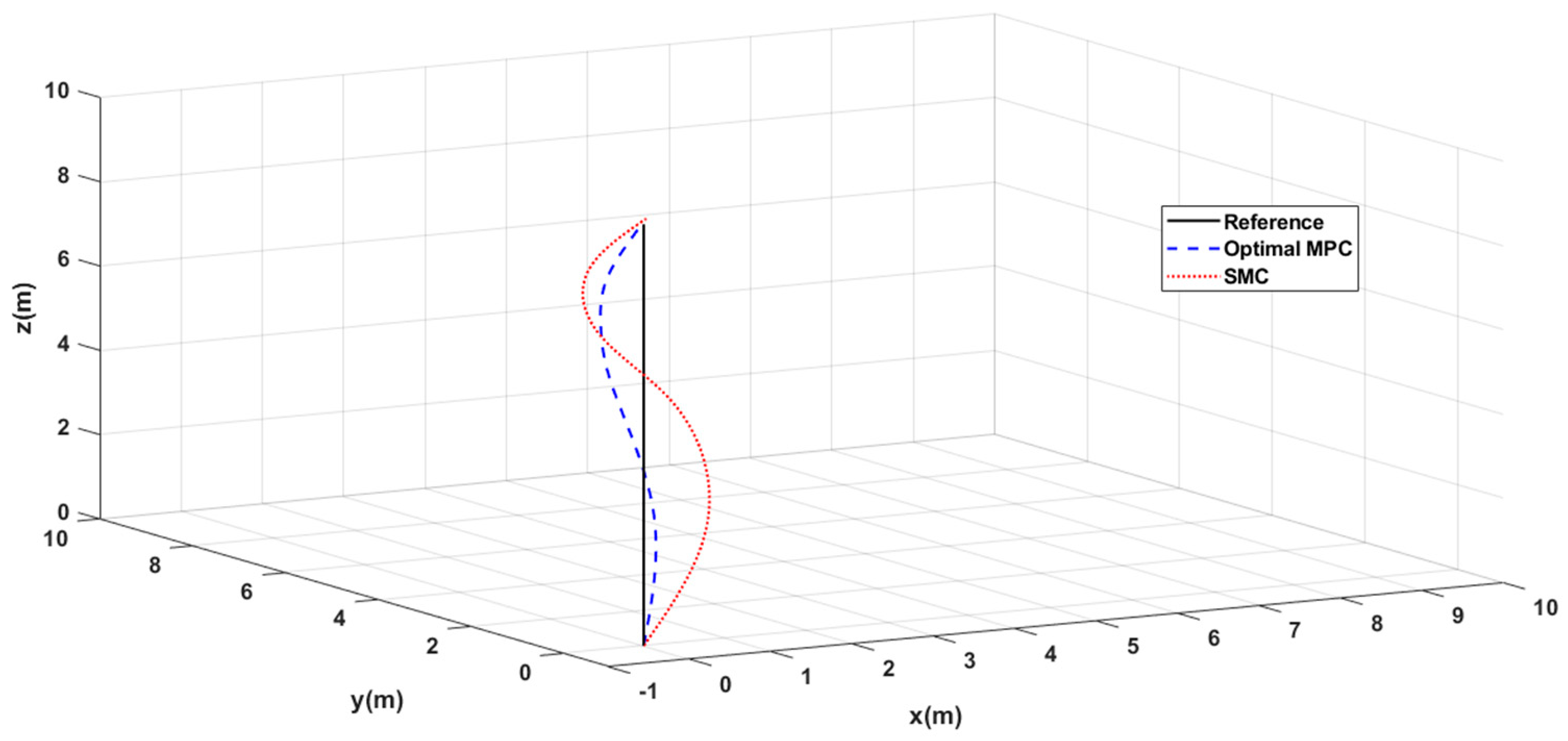
In the first scenario, it is assumed that the helicopter flies in a vertical movement from point (0, 0, 0) to point (0, 0, 10), as displayed in
Figure 1.
In
Figure 1, our proposed optimal MPC method is compared with the sliding model control method presented in [
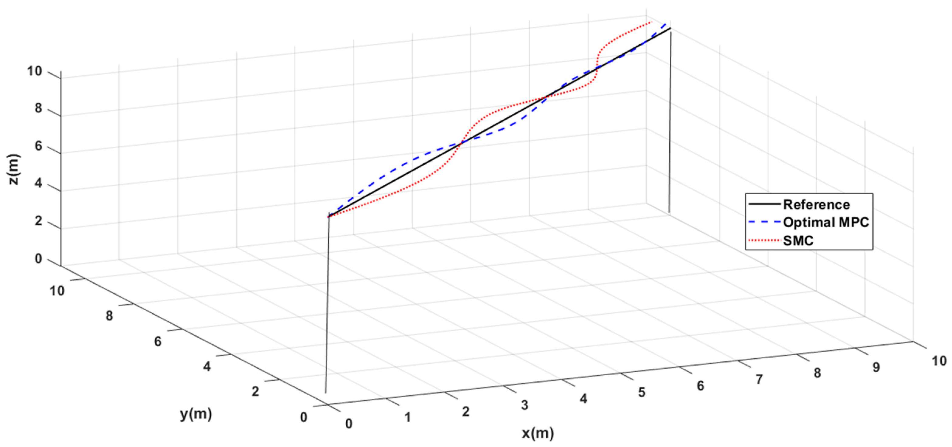
48]. As can be seen, our proposed method deviates less from the path and has a better performance. In the second scenario, the performance of the control system in the horizontal movement of the helicopter from point (0.0.10) to point (10.10.10) is evaluated, as illustrated in
Figure 2.
As can be inferred from
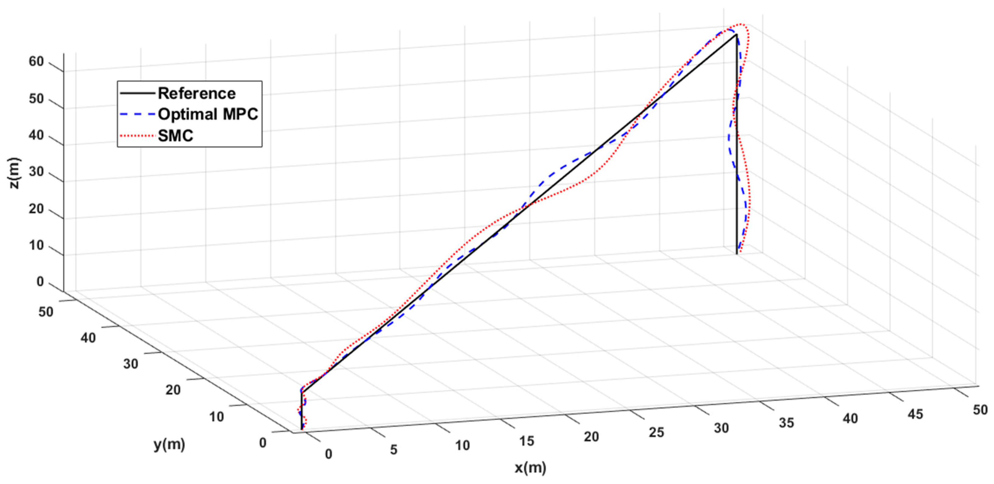
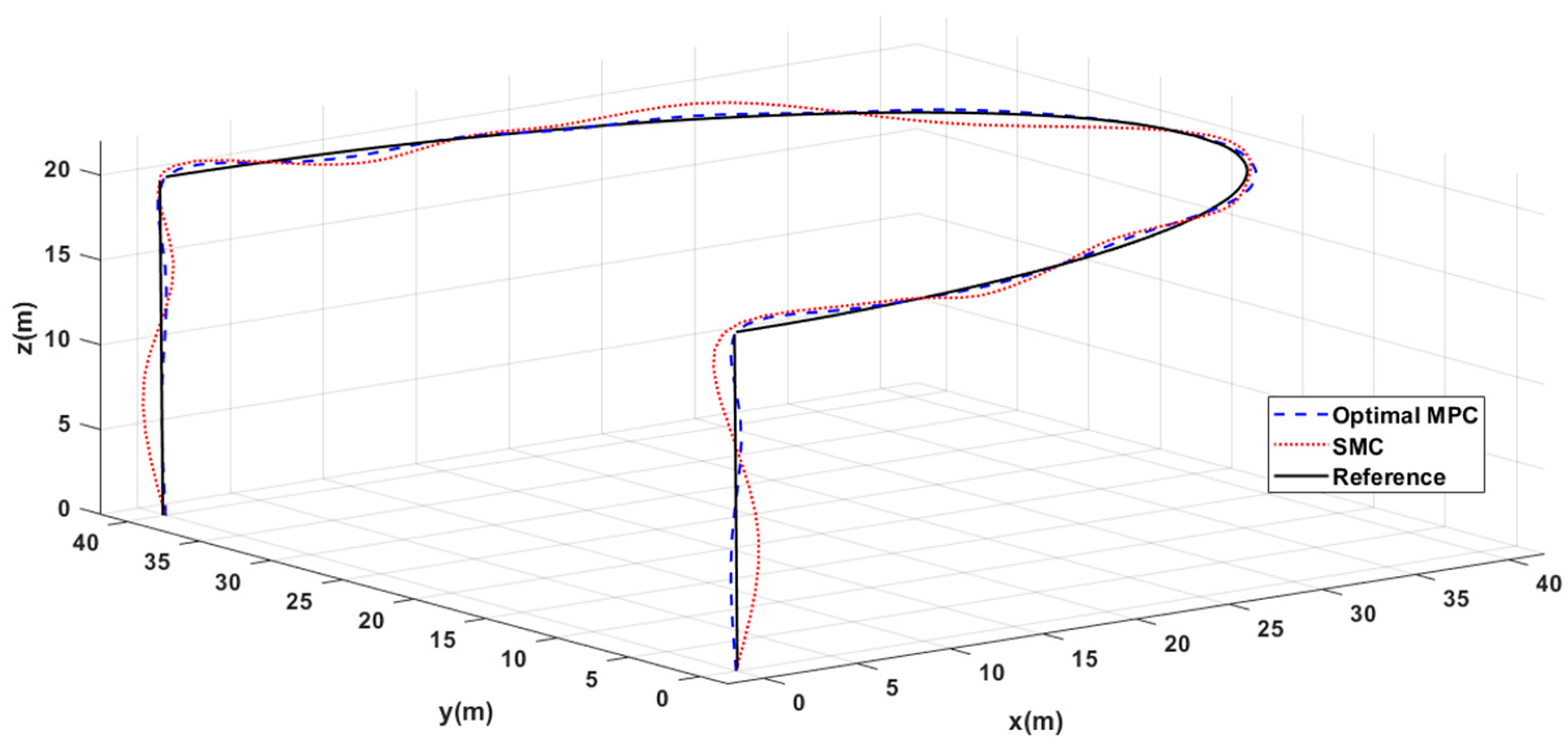
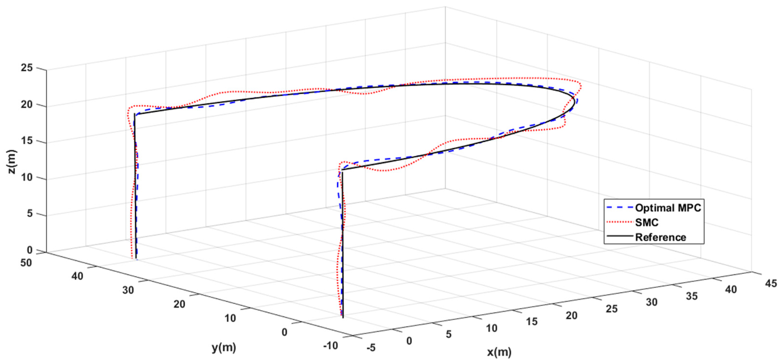
Figure 2, the performance of the optimal MPC control system is better than SMC in horizontal movement and has less deviation and error. In the third scenario, both take-off and landing are defined and there is diagonal movement. In this scenario, the helicopter first goes from point (0.0.0) to point (0.0.10) and then to point (50.50.60). In the last movement, it lands vertically at the point (50.50.0) (see
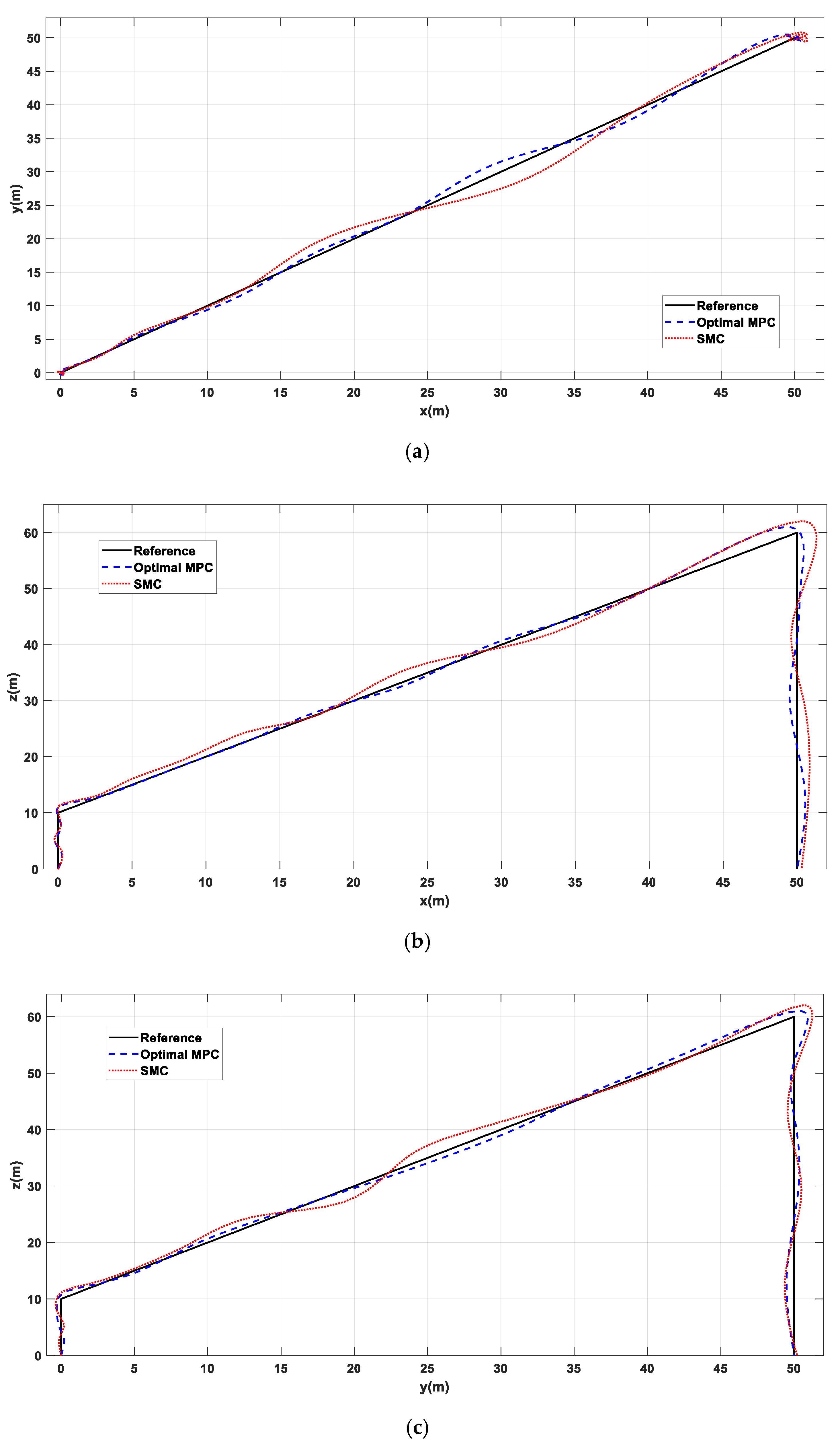
Figure 3). For more clarity, the third scenario is viewed from different angles in
Figure 4,
Figure 5 and
Figure 6.
Next, in the fourth scenario, moving along a curved path and on a semicircle is considered (
Figure 5). As can be seen in
Figure 5, the proposed method demonstrates good performance while moving on the curved path, and the control system has been able to keep the helicopter on the path. Next, the wind force is increased from 10 m/s to 15 m/s and applied to the helicopter in different directions, as shown in
Figure 6. It can be observed from
Figure 6 and
Figure 7 that the proposed control system performed very well when faced with relatively strong wind force, while the SMC method has an error of more than 3 m from the desired path.
Table 2 shows the comparison results for the proposed method against the three methods presented in other articles based on the root mean square error (RMSE) criterion.
Finally,
Table 2 shows the RMSE along the x, y, and z-axes. As can be seen, the proposed method (last column of the table) has the best performance among all methods. The reason for this problem is the use of the homotopic perturbation technique for finding the optimal analytical answer in the MPC structure.
7. Conclusions
In this paper, a new analytical method for optimal model predictive control (MPC) design was presented. In the other works, the continuous-time MPC design has finally been transformed into a discrete-time system and solved as a discrete time. On the other hand, as we know, the issue of robust control in continuous-time space is rich and strong. Therefore, these are the motivations of this paper, to propose continuous-time MPC, and it has been shown that the design of a predictive controller for continuous-time nonlinear systems is equivalent to a set of differential-algebraic equations (DAEs) with boundary conditions. By solving the mentioned sets sequentially based on homotopic perturbation, the control function and state function are obtained. Unlike methods that assume the control function at constant update intervals, this method specifies the control function and the optimal state function at all times. The presented method was tested on a small-sized helicopter, and the desired results were obtained. For this, we must have a successful design of a helicopter model. The status of the helicopter can be controlled from the following four control inputs: collective, longitudinal cyclic, lateral cyclic (main rotor), and pedal (tail rotor) commands. By obtaining the linear model in different conditions, it is possible to provide an accurate design for the helicopter. It should also be noted that, in general, helicopter control is performed using the main rotor and tail. This flying system is very sensitive to wind force, which was also addressed in the simulation. A comparison with the SMC method showed that the proposed method performs much better in all motion scenarios. The values of RMSE(x), RMSE(y), and RMSE(z) using the proposed controller are equal to 0.76, 0.71, and 0.59, respectively, which shows the superiority of this type of controller compared to other controllers.


