1. Introduction
Agriculture has assumed a significant role in contemporary society due to the increasing global population and climate change, both of which can impact the worldwide food supply. Consequently, promoting the use of technology to optimize production processes is essential for enhancing productivity, which can be vulnerable to diseases. Many crop supervision tasks require intensive labor and considerable time for expert analysis to determine the current state of crops.
Recent advancements in computer vision and artificial intelligence techniques offer promising solutions for automating the detection and classification of leaf diseases. Deep-learning methods have shown impressive performance across various crops. However, despite their effectiveness, these models often lack interpretability, making it challenging to understand the reasoning behind their decisions [
1]. Some efforts have focused on enhancing models for detecting plant diseases, with a particular emphasis on the critical role of visualization [
2]. These studies have demonstrated significant success in accurately localizing infected regions in leaf images and highlighting them with heat map overlays. Despite the promising outcomes of using eXplainable Artificial Intelligence (XAI) methods in plant disease detection, it is recognized that the field of XAI is still developing. Current explanation maps remain inadequate for fully supporting decision-making processes in this domain [
1].
Interpretability in Convolutional Neural Networks (CNNs) refers to the ability to understand, explain and attribute the decisions and predictions that the network makes. It is a crucial aspect for analyzing why a model makes certain decisions, which can be of particular importance in critical applications.
The initial visualization and interpretation works on CNNs were developed for AlexNet CNN to explore and find architectures that outperform a specific problem [
3] and to provide tools to visualize the neurons of a CNN in response to specific inputs, as well as to analyze activation patterns in response to different types of activation [
4]. Local Interpretable Model-agnostic Explanations (LIME) is then introduced as a solution based on the approximation of the original model by identifying a model that is locally faithful to the classifier on an interpretable representation, such as a binary vector indicating the presence or absence of a contiguous zone of similar pixels [
5]. On the other hand, using game theory, SHapley Additive exPlanations (SHAP) is presented as a unified measure of feature importance that is approximated by several methods and, according to its authors, best matches human intuition [
6].
In order to identify the areas of an image that represent greater importance when classifying with a CNN-based model, recent initiatives have been oriented towards methods based on class activation mapping (CAM) [
7]. One of the most representative methods is Gradient-Weighted CAM (GradCAM), which computes the local importance from the gradient of the output of a given convolutional layer (usually the last one) with respect to the class predicted by the model [
8]. GradCAM++ is presented as an enhancement to GradCAM that uses second-order gradients to improve object localization or multiple occurrences of the same class in an image [
9], while XGradCAM is presented as an improvement to GradCAM in terms of both sensitivity and conservation, where sensitivity is understood as the consistency between the removal of input features and the respective change in output, and conservation refers to the magnitude of the output equivalent to the sum of the explanation responses [
10].
Other recent examples of class activation mapping methods include HiResCAM, LayerCAM and EigenCAM. HiResCAM starts from the computation of the gradient with respect to the feature maps, and then obtains an attention map from the sum along the feature dimension of the element-wise products of the gradient and the feature maps. In order to reflect the model computations, such operations are performed when the gradients indicate that some elements of the feature map should be scaled or have their sign reversed [
11]. A variant of the latter method, GradCAMElementWise, performs an element-wise multiplication of activations with gradients and then applies a ReLU (Rectified Linear Unit) operation before summation [
12]. In LayerCAM, to obtain the class activation map of a layer, the activation value of each location in the feature map is multiplied by a weight that depends on the backward class-specific gradients; for locations with positive gradients, their gradients are used as the weight, while locations with negative gradients are assigned zero [
13]. An alternative that, according to its authors, does not rely on feature weighting such as gradient backpropagation or class relevance scoring, is the so-called EigenCAM method, which uses the principal components of the learned representations of the convolutional layers to create the visual explanations [
14].
The purpose of the methods related so far is primarily designed to illustrate which parts of an image influence the decision of a convolutional neural network. These methods have been validated on different CNNs architectures, including Inception (LIME), ResNet (SHAP, GradCAM, XGradCAM) and VGG16 (SHAP, GradCAM, GradCAM++, XGradCAM, LayerCAM, EigenCAM), with VGG16 and ResNet being the most commonly used architecture types when validating feature visualization methods using class maps. In addition to the above, it is important to keep in mind that the great diversity of methods for the identification of key regions for a classifier makes the selection of a specific method not straightforward [
15]. Also, the diversity of CNN architectures and their evolution can hinder the process of selecting and analyzing CAM-type methods.
As is well known, CNNs revolutionized computer vision research by involving feature extraction learning in training without the need for manual extraction processes [
16,
17]. In addition to this, Vision Transformers (ViT), derived from the original work on natural language processing tasks, have become a competitive option thanks to their scalability in relation to model and dataset size [
18]. Under this scenario, standard CNNs were also modernized towards the structure of a hierarchical Vision Transformer, without introducing any attention-based modules [
16]. In this way, CNNs can be as scalable as vision transformers, highlighted especially in scenarios requiring low complexity. This family has been oriented to maintain the simplicity and efficiency of CNNs and has been named ConvNext [
16], and its evolution, ConvNext2, is based on self-supervised learning [
18].
As previous research has pointed out, the quality of heat maps depends both on the methods by which they are calculated and on the performance of the classifier (model+data) [
19]. Consequently, this paper evaluates the interpretability of CNN models in the classification of coffee leaf rust. In particular, three CNN architectures (VGG16, Resnet50 and ConvNext-T) are evaluated via the seven CAM techniques both qualitatively and quantitatively using a ROAD metric.
The rest of the paper is structured as follows:
Section 2 provides the fundamentals of ConvNext networks, the selected CAM methods, and the ROAD metric.
Section 3 describes the coffee leaf dataset, the pre-trained models and the evaluation method.
Section 4 presents preliminary qualitative results for some example data and qualitative results evaluated on the test dataset. Finally,
Section 5 concludes the research results.
3. Materials and Methods
3.1. Dataset
In this study, several datasets were leveraged to aggregate a comprehensive repository of images utilized across the training, validation and testing stages of CNN model design and evaluation for the detection of coffee leaf rust. These datasets include Rocole [
27], Bracol [
28], Digipathos [
29], D&P [
30] and Licole [
31]. They encompass instances of both healthy leaves and various disease types such as rust (R: Hemileia vastatrix), leaf miner (LM: Leucoptera coffellum), phoma (P: Phoma spp), cercospora (C: Cercospora coffeicola), spider mite (RSM: Oligonychus yothersi), bacterial blight (BB: Pseudomonas syringae), blister spot (BS: Colletotrichum gloeosporioides) and sooty mold (SM: Capnodium spp).
The datasets under consideration demonstrate a notable breadth of diversity, encompassing various elements such as the presence of distractors, diverse illumination conditions (whether from artificial sources or natural sunlight), a spectrum of backgrounds and varying quantities of leaves per individual image. To prepare the dataset for analysis, meticulous preparatory procedures were executed. These tasks encompassed the precision cropping of images to isolate coffee leaves, the meticulous removal of distractors including undesired objects such as the hands of coffee growers, the exclusion of images featuring diseases other than rust, and the elimination of artificial backgrounds. The resultant dataset consists of 1686 images classified as healthy, 1723 images depicting rust, and 1928 images portraying other diseases (specifically, LM, P, C, RSM, BB, BS, and SM). The allocation for training, validation, and testing purposes involved distributing 70%, 20%, and 10% of the total images, respectively. Additionally, all the jpg images were uniformly resized to dimensions of pixels to facilitate consistent computational processing and analysis using RGB color space.
3.2. Pre-Trained Models
The CAM maps were calculated from three CNN classifiers based on VGG, ResNet, and ConvNext. The first two correspond to the two most used architectures in the evaluation of CAM methods proposed in the literature. The third one corresponds to one of the most recent architectures designed to be competitive in the context of computer vision applications. In this case, the two most widely used CNN architectures in the literature for evaluating CAM methods (VGG and ResNet) were selected, and one of the most recent pre-trained CNN architectures (ConvNext) that are widely available (e.g., in frameworks such as Tensorflow or PytTorch) for transfer learning and/or fine tuning tasks was added.
The selected architectures were used from the pre-trained models and weights available in PyTorch. The version selected in the case of VGG was VGG16, in the case of ResNet it was ResNet50, and for ConvNext the lighter version of ConvNext was used (ConvNext-T). In all three cases, the architecture classification stage was adjusted to three classes.
A fine tuning process was applied to the three pre-trained models using the training and validation subsets of the dataset explained above. This pre-training was performed on all model layers for 50 epochs, with an Adam optimizer, and learning rate decay. A checkpoint was also used to save the model, only upon an improvement in validation accuracy. The performance achieved during model fine tuning is shown in
Table 3 and
Table 4.
3.3. Selected CAM Methods
To identify the regions of importance in the decision-making of the selected classification models, class activation mapping methods were used, starting from the pioneering GradCAM scheme towards those that have made proposals to improve different aspects of the interpretation of the model output. The selected CAM schemes are listed below:
GradCAM;
XGradCAM;
HiResCAM;
LayerCAM;
GradCAM++;
GradCAMElementWise;
EigenCAM.
3.4. Evaluation Using ROAD
As discussed so far, feature attribution methods such as those based on CAM aim to identify the importance of input features for a model’s decision, within what is known as XAI. As the supply of such methods has increased, so has the need to establish techniques to evaluate these methods [
26].
This type of strategy for evaluating distribution methods is generally based on perturbing the input features that have been identified by the model as important/unimportant. Here, it is assumed that affecting the most important input features affects the performance of the model, while affecting less important features has little impact on the performance of the model [
26]. An example of such features can be the pixels of the regions identified via the attribution method (e.g., CAM).
According to the proposed methodology, the output feature map of the selected CNN architectures was evaluated using a CAM-type method. Subsequently, this CAM map was evaluated using the ROAD metric and the results were compared in order to evaluate the consistency of the selected CNN architectures. The objective here was to address the veracity/fidelity of explanation with respect to model prediction, i.e., to assess correctness, in the context of a recent classification of quantitative evaluation of Explainable AI methods [
32]. The type of evaluation method selected consisted of removing features from the input as a function of explanation (CAM) and measuring the change in predictive model output [
32].
4. Results and Discussion
This section shows the results of the application of the proposed methodology on the dataset outlined above. These results are presented first for the visual analysis of the results, and then the consolidated quantitative results for the test data are shown.
4.1. Preliminary Results (Qualitative)
In order to illustrate the differences between the regions of importance identified by the CAM methods in any of the three architectures, three examples with different levels of rust severity are shown.
Figure 3,
Figure 4 and
Figure 5 first show the original image evaluated and then the seven CAM maps (GradCAM, XGradCAM, HiResCAM, LayerCAM, GradCAM++, GradCAMElementWise, and EigenCAM) obtained with each of the three architectures.
In the case of
Figure 3, it is observed that the CAM maps obtained after applying the VGG16-based model show significant differences among them, mainly associated with the localization of the zones. However, some results show high similarity as in the case of HiResCAM, LayerCAM, and GradCAMElementWise. The results obtained using the ResNet50 architecture show a higher correlation between them, in terms of the localization and intensity of the most important zones (red tones). The differences found are mainly related to the size of the area. On the other hand, the CAM maps obtained with the ConvNext-T architecture present greater consistency among themselves in terms of localization and intensity, particularly for the first six methods shown. In this case, only the last method (EigenCAM) differs significantly from the other six.
The second test image shows a higher number of areas with rust presence (
Figure 4). First, the results for VGG16 show a great diversity of results among the different CAM methods evaluated. For example, there are methods that identify a single zone (GradCAM), methods that identify a large number of regions (HiResCAM, LayerCAM, GradCAMElementWise) or methods that identify regions outside the affected zone (GradCAM++). In the case of ResNet50-based results, from a similarity point of view, it is possible to group the results into two groups: The first identifies a small region of great importance inside the leaf, but also identifies regions outside the leaf (GradCAM, XGradCAM, HiResCAM). The second group highlights a wider area inside the leaf, covering a larger number of affected areas, but also identifies areas outside the leaf (LayerCAM, GradCAM++, GradCAMElementWise, EigenCAM). Something similar happens with the results obtained by ConvNext-T. In this case, the first group shows a small region near the leaf tip with the presence of rust, which is cataloged as being of great importance (GradCAM, XGradCAM, HiResCAM, LayerCAM). The second group identifies much of the leaf, with the leaf tip being of greatest importance, although the heat map includes areas that fall outside the leaf.
The third example (
Figure 5) shows a leaf with little presence of rust in specific areas. Again, some of the results obtained with the VGG16 architecture are similar to each other, but others vary substantially. In the case of ResNet50, the results show a similar trend to the two previous examples, where they can be framed in two groups that vary mainly by the size of the identified area. On the other hand, the results obtained with ConvNext-T show a great consistency, being very similar to each other.
4.2. Consolidated Results (Quantitative)
The proposed methodology was applied on the entire test dataset in order to evaluate the consistency of the results. In this regard, for each of the three selected CNN architectures (VGG16, ResNet50, and ConvNext-T), tests were performed with each of the seven CAM methods evaluated on the 480 images. In other words, in each architecture we have ROAD metric results for each type of CNN architecture, that is, a total of results.
Since the visual results show considerable similarities between the maps obtained with different CAM methods, especially for the ConvNext-T architecture, scatter plots were made to show the relationship between the ROAD metrics of two given CAM methods. For comparison purposes, the ROAD metric obtained with the fundamental CAM method, i.e., GradCAM, was fixed on the X-axis. In this way, the Y-axis varies with each of the other six selected CAM methods.
Figure 6 shows the scatter plots after calculating the ROAD metric on the test dataset evaluated with the VGG16 architecture. The results in this plot show that there is no correspondence between the results obtained with different CAM methods. For example, in methods such as XGradCAM, GradCAM++ or EigenCAM, it is observed that in a large number of cases, positive metric values in GradCAM correspond to negative metric values for the other CAM method and vice versa. Another aspect that stands out in this figure is that there is no proportionality between the values of the two axes, i.e., there is no relationship that illustrates that if one of the two metrics increases, the other also increases and vice versa.
Figure 7 shows the scatter plots after calculating the ROAD metric on the test dataset evaluated with the ResNet50 architecture. There is a fundamental aspect that stands out in the scatter plots of this graph: the proportionality of the results. In this case, a trend of proportionality is observed around a line of slope 1. That is, in these results, although there is a large variability around the hypothetical line of slope 1, there is a trend that as the X-axis values increase, the Y-axis values increase. This characteristic is an important difference with respect to the results obtained with VGG16.
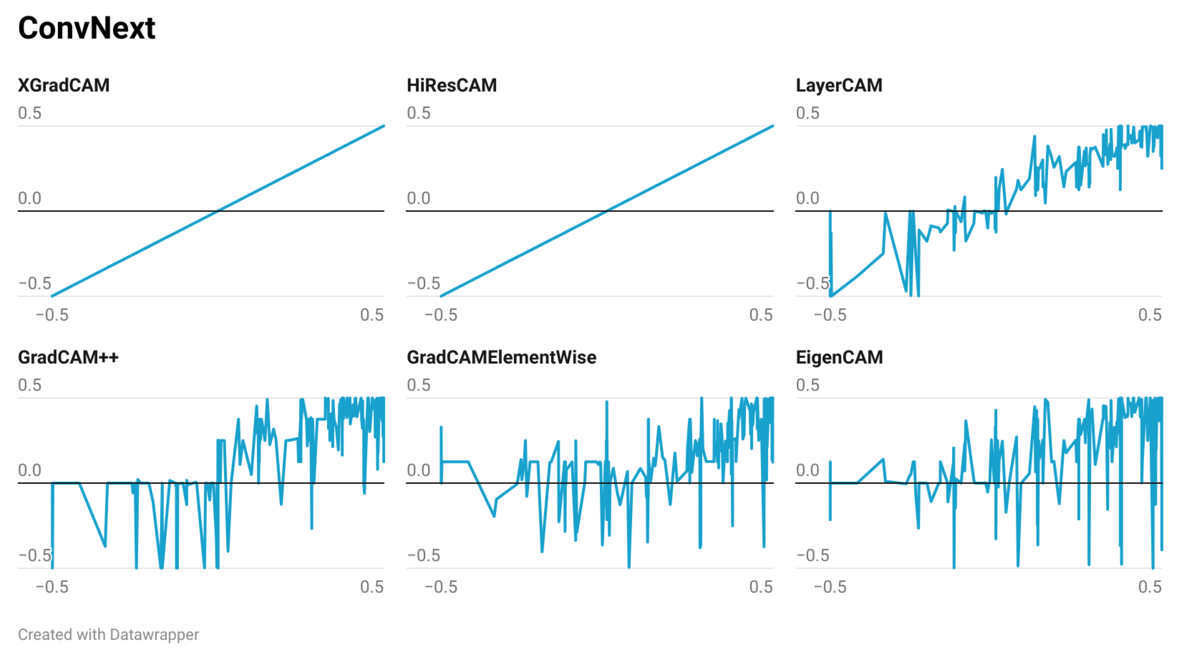
Finally,
Figure 8 shows the scatter plots after calculating the ROAD metric on the test dataset evaluated with the ConvNext-T architecture. The first thing that stands out in this plot is that the results of the XGradCAM and HiResCAM methods are highly similar to the results obtained with GradCAM. The values in these two plots, although they look like a perfect straight line, have slight differences as illustrated by the ROAD values shown in
Figure 3,
Figure 4 and
Figure 5d. However, what is corroborated here is that the importance of the regions identified through the GradCAM, XGradCAM, and HiResCAM methods have a nearly equal impact according to the ROAD metric values. Thirdly, the results obtained with the LayerCAM method show a trend proportional to the results obtained with GradCAM, i.e., it articulates around a straight line of slope 1, but with much less variation compared to the results of the ResNet50 architecture. In the case of the other three methods evaluated, the results do not present high similarities. However, the results using ConvNext-T are similar for four of the seven CAM methods evaluated, as shown in
Figure 3,
Figure 4 and
Figure 5d.
According to the results shown, the identification of regions of importance for CNN-based classifiers presents more stable results when using the ConvNext-T architecture. As shown in
Figure 3,
Figure 4 and
Figure 5d, the locations of the regions identified by all CAM methods in the ConvNext architecture are very similar to each other, and their importance in the classifier decision process evaluated with the ROAD metric shows the same trend for four of the seven CAM methods evaluated.
These results show a large variability between the regions identified by either method in two of the most commonly used architectures when evaluating CAM methods. In contrast, the regions of importance identified by the methods in the ConvNext-T architecture are highly similar in most cases.
The consistency in the output CAM maps delivered by the ConvNext architecture represents a competitive advantage thanks to the great diversity of evaluation methods that support this type of explanation. Although the present study was focused on evaluating correctness, in order to describe the fidelity of the explanation with respect to the model, by masking input features and the respective evaluation of the change in the output of the predictive model, it is possible to use heat maps to evaluate other properties of the quality of the explanation. For example, it may be possible to evaluate completeness, continuity, contrastivity, covariate complexity, compactness or coherence, as described in a recent study on Explainable AI [
32].
In terms of the type of architecture, an aspect that can make a difference has to do with the use of depth-wise convolutions. This ensures that in each operation performed by the network, information is only mixed across one dimension (either spatial or channel), but not both at the same time [
16]. This validation can be further studied by considering architectures that use this type of convolution such as Xception-[
33] or MobileNet [
34]-based architectures.
Another aspect to consider here has to do with the type of data or specific problem on which the proposed methodology has been evaluated. Although the present study has focused on coffee leaf rust classification, a first alternative may be to consider extending these results to the detection of rust on other crops, or other leaf diseases. Beyond this, it is possible to apply similar studies on other classification problems or even object detection.


