Multi-Objective Optimized GPSR Intelligent Routing Protocol for UAV Clusters

Abstract

Unmanned aerial vehicle (UAV) clusters offer significant potential in civil, military, and commercial fields due to their flexibility and cooperative capabilities. However, characteristics such as dynamic topology and limited energy storage bring challenges to the design of routing protocols for UAV networks. This study leverages the Deep Double Q-Learning Network (DDQN) algorithm to optimize the traditional Greedy Perimeter Stateless Routing (GPSR) protocol, resulting in a multi-objective optimized GPSR routing protocol (DDQN-MTGPSR). By constructing a multi-objective routing optimization model through cross-layer data fusion, the proposed approach aims to enhance UAV network communication performance comprehensively. In addition, this study develops the above DDQN-MTGPSR intelligent routing algorithm based on the NS-3 platform and uses an artificial intelligence framework. In order to verify the effectiveness of the DDQN-MTGPSR algorithm, it is simulated and compared with the traditional ad hoc routing protocols, and the experimental results show that compared with the GPSR protocol, the DDQN-MTGPSR has achieved significant optimization in the key metrics such as the average end-to-end delay, packet delivery rate, node average residual energy variance and percentage of node average residual energy. In high dynamic scenarios, the above indicators were optimized by 20.05%, 12.72%, 0.47%, and 50.15%, respectively, while optimizing 36.31%, 26.26%, 8.709%, and 69.3% in large-scale scenarios, respectively.

1. Introduction

UAVs are widely used in military and civil applications, including public protection and disaster relief [1], surveillance and reconnaissance [2], border monitoring [3], autonomous tracking [4], search and destruction operations [5], public safety [6], homeland security [7], fisheries monitoring [8], transportation monitoring [9] and network relay [10]. Compared to a single unmanned platform, UAV clusters offer an efficient solution for complex missions due to their high flexibility and distributed deployment, allowing for extended operation areas and enhanced capabilities in monitoring, reconnaissance, and multi-target execution.

Due to restricted communication distances, most source nodes cannot communicate directly with the destination node and must relay information through neighboring nodes. In semi-autonomous or autonomous states, the communication capability of UAV clusters is mainly constrained by dynamic topology and limited energy storage, posing challenges for designing routing protocols. Key challenges include highly dynamic topology, unstable link connections [11], limited transmission range and on-board energy [12], and the effects of network size and node density [13].

UAV clusters move unpredictably and randomly for extended periods, making it crucial to develop intelligent routing protocols that quickly adapt to network changes. Effective routing decision-making is vital for improving data delivery rates and reducing network delay, optimizing overall performance.

Traditional routing protocols are categorized into topology-based and geolocation-based protocols. Topology-based protocols include (1) proactive routing protocols: examples are Destination-Sequenced Distance-Vector (DSDV) [14] and Optimized Link State Routing (OLSR) [15], which are slow to react to dynamic topologies, leading to delays, routing loops, and blind routes [16]. (2) Reactive Routing Protocols: examples are Dynamic Source Routing (DSR) [17] and Ad Hoc on-Demand Distance Vector Routing (AODV) [18]. In large UAV networks, these may face routing failures, increased delay, and high bandwidth consumption. (3) Hybrid Routing Protocol (HRP): this combines proactive and reactive approaches, maintaining different routing tables for area and out-of-area members [19]. However, they face higher computational complexity and overhead due to complex clustering processes [20].

Geolocation-based routing protocols differ from topology-based protocols by not relying on complex routing tables but using the location information of destination nodes and neighbors for path selection. This makes them more suitable for highly dynamic UAV networks. A typical geolocation routing protocol is Greedy Perimeter Stateless Routing (GPSR) [21], which relies on instantaneous location information for better performance in dynamic environments. However, GPSR is sensitive to node density, and GPSR only focuses on distance information when forwarding without considering factors such as node load, which may lead to problems such as link congestion, thus reducing network performance.

Recently, optimizing traditional routing protocols with machine learning algorithms has become a major research focus. These protocols adaptively learn the environment state, predict topological changes, and improve communication quality and energy efficiency. The main categories are reinforcement learning (RL)-based, deep learning (DL)-based, and deep reinforcement learning-based (DRL).

The main contributions in this study are as follows:

• Mathematical modeling of multi-objective routing optimization problem: combines the multi-objective optimization mechanism of DDQN, transforming the route forwarding process into a Markov decision process (MDP) and modeling the multi-objective routing optimization problem by comprehensively considering multiple routing performance metrics in a mixed-objective way.
• DDQN-based GPSR optimization: uses DDQN to improve the traditional GPSR routing mechanism, constructing a DDQN network model to solve the routing problem.
• NS-3-based implementation and validation: combines the NS-3 network simulator with an AI framework via the NS3-AI interface to integrate and validate the DDQN-MTGPSR intelligent routing protocol, showing superior performance in large-scale, highly dynamic networks compared to other routing protocols.

The rest of the paper is structured as follows. Section 2 reviews related research on UAV cluster routing protocols. Section 3 presents the mathematical modeling of the routing optimization problem. Section 4 describes the design process of the DDQN-MTGPSR protocol. Section 5 covers the simulation experiments and analysis. Section 6 summarizes the research and suggests directions for future improvement.

2. Related Work

2.1. Improved Routing Protocols Based on RL

The core advantage of the RL algorithm lies in the design of its abstract formulation, which enables the algorithm to be independent of the specific prediction of topology and the precise estimation of channel conditions, endowing the algorithm with strong versatility and adaptability, and showing excellent application advantages under dynamic or unknown network conditions.

Recent literature [22] has introduced Q-Learning (QL) into routing protocol studies, proposing the Q-Routing Protocol, which outperforms non-adaptive algorithms based on counting shortest paths and routes efficiently even with changing network loads. Study [23] proposed the Q-Learning-based Geographic Routing Protocol (QGeo). Experiments show that QGeo outperforms traditional location-based protocols in terms of delivery rate and network overhead in high-mobility UAV scenarios. However, QGeo does not balance exploration and exploitation strategies to find better relay UAVs, nor does it consider energy consumption. Further literature [24] proposed Reward Function Learning for QL-Based Geographic Routing Protocol (RFLQGEO). RFLQGEO offers fewer retransmissions, lower average end-to-end delay, and a higher delivery rate than QGeo. Its limitations include not considering mobility control mechanisms, exploration and exploitation methods, or energy consumption. Study [25] designed the Geolocation Ad Hoc Network (GLAN) routing system using geolocation information and developed the Adaptive GLAN (AGLAN) system. This system applies RL to adapt to changing environments and introduces a pseudo-attention function in RL, improving learning efficiency. However, it only considers geolocation conditions during design.

2.2. Improved Routing Protocols Based on DL

DL predicts the future state of a network by training with sample data to avoid connection failures and congestion, making it suitable for studying complex network routing protocols [26].

A distributed routing algorithm based on local geolocation information has been proposed in the literature [27], which constructed a dataset using historical flight data to train Deep Neural Networks (DNN), considering end-to-end delay, network capacity, and path lifetime in the optimization process. Simulation results show that this DL-assisted routing algorithm outperforms existing location-based protocols in these metrics, though its computational complexity and power consumption increase due to the Pareto frontier problem in DL. Study [28] utilized the learning ability of neural networks and the explanatory ability of fuzzy logic to find routing next hops, optimize quality of service (QoS) metrics, and improve network performance. The algorithm considers distance, movement trends, and queuing delays but not energy consumption. Experiments based on real historical flight data demonstrate significant improvements in end-to-end delay and transmission rate.

2.3. Improved Routing Protocols Based on DRL

In large-scale, highly dynamic unmanned clusters networks, reliable communication routing needs to meet the requirements of efficient energy utilization, low latency, node load balancing, etc. to achieve reliable data transmission. Since traditional single-objective optimization is difficult to comprehensively weigh various indicators that affect routing performance, such as link quality, latency, energy consumption, distance, and hole probability, multi-objective routing optimization problem design based on the above indicators can achieve the purpose of comprehensively improving network performance. In

Table 1. Comparison of consideration factors for different routing protocols.

Routing Protocol	Protocol Type	Geographical Position	Energy Consumption Factor	Routing Hole	Transmission Speed/Delay Factor	Relative Moving Trend
Q-Routing [22]	RL	✓	✗	✗	✗	✗
QGEO [23]	RL	✓	✗	✗	✓	✗
RFLQGEO [24]	RL	✓	✗	✗	✓	✓
GLAN [25]	RL	✓	✗	✗	✗	✗
DL-Aided Routing [27]	DL	✓	✗	✗	✓	✗
NF-Routing [28]	DL	✓	✗	✗	✓	✓

, this paper classifies and summarizes the characteristics of the above-mentioned improved geolocation routing protocols and intuitively shows the indicators covered and not covered in the design process of each routing protocol. In

Table 2. A summary of the advantages and disadvantages of the application of RL and DL concepts in large-scale and highly dynamic unmanned clusters.

Type	Routing Protocol	Application Scenario	Application Advantage	Application Disadvantage
RL-Routing	[22,23,24,25]	Large-scale and highly dynamic unmanned cluster networks	Abstract formulation design, Strong versatility and adaptability, Applications on dynamic or unknown networks.	Not applicable to large-scale networks, Application of multiple objectives in routing problem.
DL-Routing	[27,28]		Explore the relationship between environmental characteristics and optimal paths.	Network architecture design training datasets, Overfitting issues.

, this paper classifies and summarizes the advantages and disadvantages of the improved routing protocols based on RL and DL ideas when applied to large-scale, highly dynamic unmanned clusters.

Currently, most UAV cluster routing protocols based on RL use the QL algorithm, but they have several shortcomings in UAV networks: (1) As the number of network nodes increases, the state and action spaces expand significantly, making it time-consuming to learn large Q-tables and difficult to ensure algorithm convergence, which hinders adaptation to large-scale network scenarios. (2) Most current routing protocols rarely consider multiple performance indicators such as distance, energy consumption, delay, and link quality, limiting their effectiveness in practical applications.

In addition to RL techniques, routing protocols can explore the relationship between local network topology, geographic location, and link states using DL. However, further research is needed to address challenges such as designing appropriate deep network architectures, constructing relevant training datasets, and addressing potential overfitting issues.

The DRL algorithm, developed from RL, combines DL’s perception capabilities with RL’s decision-making abilities. DRL-based dynamic routing algorithms can better perceive the changing multidimensional parameters of the environment, establish a mapping between environmental data and routing decisions, and are ideal for learning dynamic network topologies and traffic conditions [12]. This study uses an optimized DRL algorithm, Deep Double Q-Learning Network (DDQN), to design a Multi-Objective Optimized GPSR-based protocol, termed DDQN-MTGPSR.

3. Mathematical Modeling of Multi-Objective Routing Optimization Problems

Traditional multi-objective routing optimization problems are often solved by meta-heuristic algorithms such as Simulated Annealing (SA), Genetic Algorithm (GA), and Particle Swarm Optimization (PSO). However, these algorithms do not guarantee finding an approximate optimal solution and face issues like delayed convergence and high computational complexity [29], especially in large-scale, highly dynamic, and complex network environments [30].

In recent years, the DRL algorithm has demonstrated excellent performance in solving multi-objective optimization problems, particularly for large-scale and highly dynamic UAV cluster networks, DRL has emerged as an effective solution for multi-objective routing optimization, capable of adapting to complex and changing environments [31].

3.1. Deep Double Q-Learning Network

The sequential behavioral decision problem of the DDQN algorithm is defined by the MDP, which introduces an Agent that learns a value function, which is associated with Bellman’s equation, and together, guide the agent’s decision-making process. In this study, we use this model to model the routing process of UAV clusters. MDP consists of the tuple $\left\{S,A,P,R\right\}$, where S, A, P, and R denote the state space, action space, state transfer probability, and the reward function, respectively. The agent takes an action $a$ at $s$ according to the policy $\pi$. The environment sends a reward $r$ to the agent based on the agent’s action $a$ and transfers to the next state $s’$. The agent acquires the experience tuple$e=(s,a,r,s^{\prime })$. The goal of the intelligence is to learn the optimal strategy to maximize the desired reward.

The DDQN algorithm is a variant of Q-learning, a non-strategic RL algorithm based on model-free values, based on the action value function$Q(s,a)$, iteratively updating the Q-value function using Bellman’s equation and gradually approximating the optimal value function to obtain higher rewards. The Bellman’s optimal equation for QL is:

$$Q^{*}\left(s,a\right)=r\left(s,a\right)+\gamma {\displaystyle \sum }_{s^{\prime }\in S}P(s^{\prime }|s,a)\underset{a\in A}{\text{max}{Q}^{*}\left(s^{\prime },a^{\prime }\right) }$$

(1)

where $(s,a)$ denotes the reward value for taking action a under s, $\gamma$ denotes the discount factor, and $P\left(s^{\prime }\right|s,a)$ denotes the execution of action $a$ the probability of transferring from states to s’ afterward. $Q^{*}(s,a)$ is approximated by the following equation:

$$Q(s,a)\leftarrow Q(s,a)+\alpha [r+\gamma Q(s^{\prime },a^{\prime })-Q(s,a\left)\right]$$

(2)

where $\alpha$ represents the learning rate. The optimal policy ${\pi }^{*}$ is the policy that makes $Q(s,a)$ approach $Q^{*}(s,a)$.

The DDQN uses a deep neural network to approximate $Q(s,a)$, which gradually learns an accurate action value function to select the optimal action by introducing a deep neural network, defining an empirical playback region, computing the target value, and updating the network parameters in a gradient descent inverse manner.

(1) Experience playback: the experience playback mechanism works by storing experiences in order to compose a sequence of experiences $D=\{e_1,e_2,...e_n\}$. During training, experience samples are randomly selected from D randomly selected experience samples and adopts the gradient descent algorithm when updating network parameters, which improves the efficiency of utilizing historical data and reduces data correlation.

(2) Target network $w’$: DDQN utilizes a deep neural network to approximate the action value function, which is denoted as $Q(s,a;{\theta }_i)$, where ${\theta }_i$ denotes the parameters of the network at the i-th iteration. The optimization objective value is $y^{DDQN}=r+\gamma Q\left(s^{\prime },\underset{a}{\mathrm{a}\mathrm{r}\mathrm{g}\mathrm{m}\mathrm{a}\mathrm{x}}Q\left(s^{\prime },a;{\theta }_i\right);{{\theta }_i}^{-}\right),$the objective value is calculated by the target network $w’$ and evaluation network $w$, $s’$is the next state, $a’$ denotes the possible actions, and ${{\theta }_i}^{-}$ is the parameter of the target network. Throughout the training process, the DDQN updates the network parameters inversely by minimizing the loss function, and the loss function at the i-th update is as follows:

$$L_i({\theta }_i)=E_{(s,a,r,s^{\prime })}\left[{(y^{DDQN}-Q(s,a;{\theta }_i\left)\right)}^2\right]$$

(3)

For the parameters (weights) of the (3), the partial derivation of the parameters (weights) is obtained by (4):

$${\nabla }_{{\theta }_i}{L}_i\left({\theta }_i\right)=E_{(s,a,r,s^{\prime })}\left[\right(y-Q(s,a;{\theta }_i)\left){\nabla }_{{\theta }_i}Q\right(s,a;{\theta }_i\left)\right]$$

(4)

Target Network $w’$ and evaluation network $w$ have the same network structure, where the network parameters ${\theta }_i$ of the evaluation network are used to update the parameters ${\theta }_i$ of the target network after every N iterations.

3.2. MDP Modeling of the Routing Forwarding Process

(1) State space: let the state space of the node i where the packet is currently located be $s_t$, $s_t=\{s_{1,t},s_{2,t},...,s_{n,t}\}$, where $s_{j,t}$ denotes the state information of the neighboring node $j$of $i$ at the moment$t$, and $n$ denotes the number of all neighbor nodes of this node, and this study defines $s_{j,t}$ as:

$$s_{j,t}=\{SN{R}_{i,j},E_j^{grade},T_j^{wait},d_{i,dst},d_{j,dst},P_{ho{p}_2},{\mathrm{c}\mathrm{o}\mathrm{s}}_{j,d}\},j\in NBR(i)$$

(5)

where $NBR\left(i\right)$ denotes the set of neighbors of the node; $SN{R}_{i,j}$ denotes the signal-to-noise ratio (SNR) between the current node $i$ and the neighbor node $j$, reflecting the link quality; $E_j^{grade}$ denotes the residual energy level of the candidate neighbor node; $T_j^{wait}$ denotes the expected total waiting delay of the packet in the neighbor node $j$; $d_{i,dst}$ indicates the distance between node i and destination; $d_{j,dst}$ denotes the distance between the neighbor node j and destination node; $P_{ho{p}_2}$ denotes the probability of a routing hole occurring in neighboring node j; ${\mathrm{c}\mathrm{o}\mathrm{s}}_{j,d}$ indicates $j’s$ relative movement trend with respect to the destination node.

• Signal-to-noise ratio (SNR)

$SNR$ is an important indicator of the quality of a communication link. For wireless communication environments, a higher SNR indicates better signal quality. It is assumed that the energy of the received signal $S\left(k\right)$outside the packet $k$ acceptance interval is 0. The received power of the signal is derived from the path loss propagation model as well as the signal transmit power. The calculation is based on the Friis free-space propagation model (Friis), which takes into account the attenuation of the signal with increasing propagation distance [32]. The calculation process is shown in (6):

$$P_l(d)=P_l(d_0)+n10{\mathrm{l}\mathrm{o}\mathrm{g}}_{10}({\displaystyle \frac{d}{d_0}})$$

(6)

where $P_l\left(d\right)$ is s the received power at distance d, is the reference distance, n is the path loss exponent (usually within 2 to 6), $d_0$ is the reference distance, $P_l\left(d_0\right)$ is the received power at the reference distance of $d_0$ ($d_0$ usually set to 1 m), is the reference distance, and d is the actual distance between the receiver and the transmitter. Based on the Friis propagation model to define the calculation method of the reference distance received power $P_l\left(d_0\right)$:

$$P_l(d_0)={\displaystyle \frac{P_t{G}_t{G}_r{\lambda }^2}{16{\pi }^2{d}_0^{2}L}}$$

(7)

where $P_t$ denotes the signal transmit power, $G_t$ denotes the gain of the transmit antenna (default value 1 dBm), $G_r$ denotes the gain of the receive antenna (default value 1 dBm), $\lambda$ denotes the radio carrier wavelength, $d_0$ denotes the reference distance, and $L$ denotes the system loss (default value 1).

The receiving end utilizes the formula (8) to calculate $SNR\left(k\right),$ the signal-to-noise ratio of the packet k:

$$SNR(k)=10\mathrm{l}\mathrm{g}({\displaystyle \frac{S_k}{N_i\left(k\right)+N_f}})=10\mathrm{l}\mathrm{g}({\displaystyle \frac{P_l\left(k\right)}{N_i\left(k\right)+N_f}})$$

(8)

where $N_f$ represents the noise floor, which is a characteristic constant of the receiving circuit. $N_i\left(k\right)$ represents the interference noise, which is the sum of the energies of all other signals received on the same channel. $N_i\left(k\right)$ can be expressed as:

$$N_i(k)={\sum }_{m\ne k}S\left(m\right)$$

(9)

The base noise of the receiver needs $N_f$ to take into account the thermal noise and the non-ideality of the receiver, which is calculated as follows:

$$N_f=NF\cdot Nt$$

(10)

where $NF$ is the noise figure, $Nt$ is the thermal noise power. $Nt=kTB$, $k=1.3803\times {10}^{-23}$ is the Boltzmann constant in J/K, T = 290 K is the temperature, and B is the channel width in Hz.

• Residual energy percentage

Energy utilization is an important performance indicator for the operation of unmanned clustered networks, and optimizing the energy consumption problem is critical. In order to balance the energy consumption of the nodes within the network, this study considers adding the residual energy share metrics of the candidate neighbors in the next-hop selection process $E_j^{grade}$, which is calculated as described below:

$$E_j^{grade}={\displaystyle \frac{E_{re{m}_j}}{E_{ini{t}_j}}}$$

(11)

where $E_{re{m}_j}$ denotes the remaining energy of neighbor node j and $E_{ini{t}_j}$ denotes the initial energy of neighbor node j, and the ratio of the two can evaluate the energy consumption after a period of time.

• Expected total waiting delay within the node

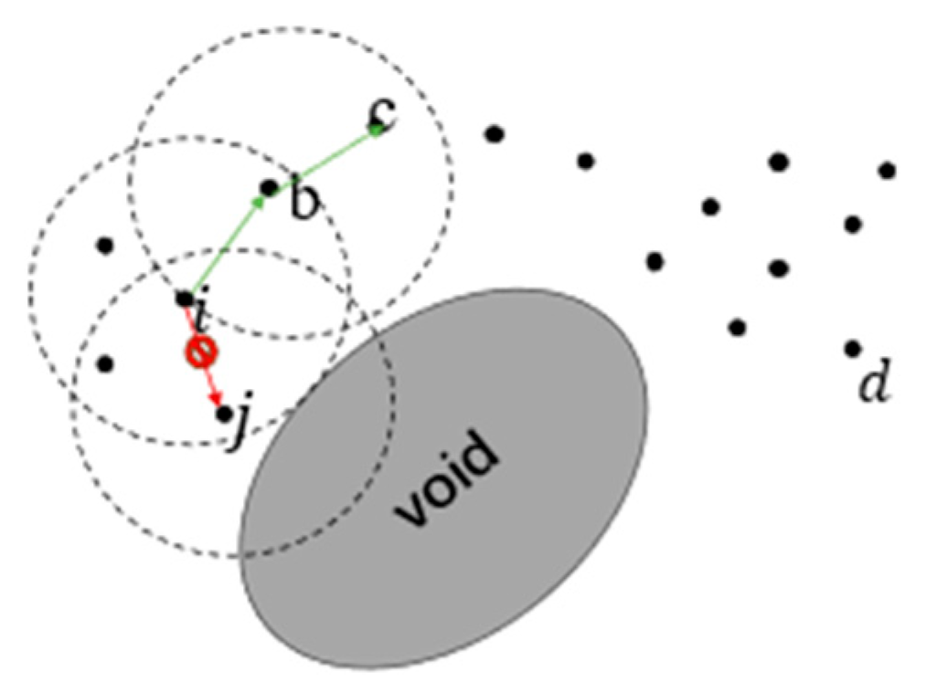
In this study, we approximate the expected total waiting delay of a packet in the node j, representing that if the node i chooses to send the data packet to neighbor j, the packet will be processed after the waiting time of $T_j^{wait}$. The computational procedure of $T_j^{wait}$ is developed as follows:

$$T_j^{wait}=T_j^t+T_j^q$$

(12)

where $T_j^t$ denotes the transmission delay of all packets in the MAC layer of the candidate neighbor node j, $T_j^q$ denotes the expected queuing delay in the IP layer. The processing delay and the propagation delay are not considered in this study since the processing delay can be of a subtle or even lower order of magnitude, while the propagation delay in UAV clusters on the order of hundreds of meters is on the order of nanoseconds. The calculation of $T_j^t$ and $T_j^q$are shown as (13) and (14):

$$T_j^t={\displaystyle \frac{DataSiz{e}_p}{DataRat{e}_{dev}}}$$

(13)

$$T_j^q=T_q^{avg}\cdot su{m}_{pkt}$$

(14)

where $DataSiz{e}_p$ indicates the length of all packets in the link layer in bits. $DataRat{e}_{dev}$ denotes the device's data transfer rate. Further, to estimate the queuing delay of all packets in j , we utilize the total number of packets in the queue $su{m}_{pkt}$ and the average queuing delay of packets $T_q^{avg}$. Further, this study estimates the queuing delay by a method of calculating the dynamic average queuing delay based on a fixed window.

This method maintains a fixed number of packet counts $N$ as an observation window and calculates the average queuing delay within the current window $T_q^{avg}$. Once the total number of packets counted is greater than the current window $N$, it is necessary to clear the state for the monitoring of the next window, including the reset of the cumulative value of the queuing delay and the value of the queuing packet count, this average delay calculation is defined as follows (15). This average delay calculation is defined as shown:

$$T_q^{avg}=\frac{{{\displaystyle \sum }}_{i=1}^{count}{t}_i^{De}-t_i^{En}}{count}$$

(15)

where $count$ indicates the total number of queued packets in the window at the current moment $(count\le N)$, $t_i^{De}$ denotes the outgoing queue moment of the i-th packet, $t_i^{En}$ denotes the moment when the i-th packet enters the queue. It should be noted that every time a packet is queued out of the buffer, the average delay is updated.

• Routing void possibilities $P_{ho{p}_2}$,

  $$P_{ho{p}_2}=d_{(i^{hop2},dst)}^{\mathrm{m}\mathrm{i}\mathrm{n}}/d_{i,dst}$$

  (16)

As (16) shows, where $d_{(i^{hop2},dst)}^{\mathrm{m}\mathrm{i}\mathrm{n}}$ denotes the shortest distance of a two-hop neighbor node from the destination node estimated by the current node $i$ based on the perimeter topology information of the forwarding node $j$. In this study, we utilize the method in literature [33] to calculate the surrounding topology information NBT of all the nodes and broadcast it periodically with the HELLO beacon. The nodes receiving the message will estimate $d_{(i^{hop2},dst)}^{\mathrm{m}\mathrm{i}\mathrm{n}}$ based on the NBT and further get $P_{ho{p}_2}$.

If $P_{ho{p}_2}>1$, it means that once the current node $i$ chooses $j$as the next hop, node $j$ is likely to have the routing hole problem. The principle is shown in Figure 1, if node $i$ chooses the neighbor j as the next hop ($j$ is closest to the destination), when the packet is forwarded to $j$, there is a high probability of a routing hole after the packet is forwarded. Therefore, calculating $d_{(i^{hop2},dst)}^{\mathrm{m}\mathrm{i}\mathrm{n}}$ in node $i$ based on $j$‘s neighboring topology information can prevent data from being forwarded to node$j$ and falling into a routing hole.

• Relative movement trends ${\mathrm{c}\mathrm{o}\mathrm{s}}_{j,d}$.

${\mathrm{c}\mathrm{o}\mathrm{s}}_{j,d}$ indicates the relative movement trend of the candidate neighbor node with respect to the destination node dst, which is defined by the computation method as Equation (17) shown:

$${\mathrm{c}\mathrm{o}\mathrm{s}}_{j,d}={\displaystyle \frac{{\stackrel{⃑}{V}}_j\cdot \stackrel{⃑}{l_j{l}_{dst}}}{‖{\stackrel{⃑}{V}}_j‖‖\stackrel{⃑}{l_j{l}_{dst}}‖}}$$

(17)

where ${\stackrel{⃑}{V}}_j$ denotes the speed vector of node j, $\stackrel{⃑}{l_j{l}_{dst}}$ denotes the distance vector from the node j to the destination node.

(2) Action space: $A=\{n_1,n_2,n_3....n_n\}$, denotes the set of all neighbor nodes of the current node i, where $n_j$ denotes the j-th neighboring node, and n denotes the total number of nodes. If there is a packet forwarding requirement for the current node, the next hop node needs to be decided as routing in this set.

(3) Transfer probabilities: DDQN belongs to a model-free approach, which does not require explicit knowledge of the state transfer probabilities of MDP, and can learn the optimal policy through interaction with the network environment.

(4) Reward function R: the reward mechanism is an important factor in refining the strategy. If the chosen action leads to a weak reward, the agent can choose other actions in the future under the same conditions to obtain other reward possibilities [34].

In this study, we give all the objective metrics of the multi-objective routing optimization problem in the reward mechanism of DDQN-MTGPSR to provide behavioral guidance for routing decisions [35]. The reward mechanism $r_{i,j}$ of DDQN-MTGPSR is as (19) shown:

$$r_{i,j}=\{\begin{array}{ll}{k}_1{e}^{-T_j^{wait}}+k_2{e}^{-P_{ho{p}_2}}+k_3{e}^{-d_{j,dst}}+k_{4}SN{R}_{i,j}+k_5{E}_j^{grade}& ,j is’t dst\\ r_{\max }& ,jisdst\end{array}$$

(18)

where $k_1$ to $k_5$ are the weight values and ${\sum }_{i=1}^5{k}_i=1,k_i>0$. Finally, the algorithm will tend to select the next hop node with less delay, better link quality, more energy left, lower possibility of routing hole, and shorter distance to the destination. In this study, the Min-Max Scaling method is chosen to normalize the state eigenvalues.

4. DDQN-MTGPSR Protocol Design

4.1. Broadcast Beacon and Routing Table Optimization

DDQN-MTGPSR periodically broadcasts beacons containing the local node’s ID, location, residual energy, mobility mode (speed and direction), estimated total waiting delay, and neighboring topology information (NBT). Upon receiving a beacon, a node calculates the SNR and parses the packet, storing the information in its routing table, referred to as $RT$in this study.

Table 3. Improved GPSR routing table RT.

Field 1	Field 2	Field 3	Field 4	Field 5	Field 6	Field 7	Field 8
${ID}_1$	coordinate (geometry)	moving model	delay	energy	${NBT}_1$	${SNR}_{1,i}$	timestamp
${ID}_2$	coordinate (geometry)	moving model	delay	energy	${NBT}_2$	${SNR}_{2,i}$	timestamp
......	......	......	......	......	……	……	......
${ID}_n$	coordinate (geometry)	moving model	delay	energy	${NBT}_n$	${SNR}_{n,i}$	timestamp

is the improved GPSR routing table RT, which needs to be maintained, and if no broadcast packet is received from a neighbor node for a period longer than T, the neighbor information is removed from the routing table.

4.2. DDQN Network Construction

Figure 2 demonstrates the application of the DDQN model to the UAV cluster routing decision problem, reflecting the interaction between the model and the network environment. The agent uses the current network state $s_t$ and selects the next hop routing node based on the policy $\pi$ to select the next-hop routing node, and the network state is further transformed to $s_{t+1}$ after the environment performs the action and gives a reward $r_t$.

If there is a demand for packet forwarding in the current node, it needs to get the state information of each neighbor as shown in (5) according to the destination node information stored in the packet and the routing table of this node, and integrated into the state space $s_t$. Each network of DDQN consists of input layer $IN$, hidden layer $Hd$, and output layer $L_o$. The hidden layer consists of a convolutional layer $Conv$ and two fully connected layers ${Fc}_1$ and ${Fc}_2$. If the total number of neighbor nodes is $N_{nb}$, then the input data is a two-dimensional matrix of size $N_{nb}\times 7$, where 7 is the number of state eigenvalues.

Convolutional layer for hidden layer $Conv:$ The size of the convolutional kernel is $2\times 2$, stride is 1, and no padding in both height and width directions. The convolutional layer has a total of $N_{nr}=(N_{nb}-1)\times (n_{FeatureMap}-1)\times n_{FeatureMap}$ neurons, where $n_{FeatureMap}$ denotes the number of feature maps (equals 7). Fully connected layers ${Fc}_1$ and ${Fc}_2$: the number of neurons of ${Fc}_1$ can be taken in the interval range of $[4N_{nb},6N_{nb}]$, the number of neurons of ${Fc}_2$ can take the value of $N_{nb}$. Each fully connected layer uses a rectified linear unit (ReLU).

Input $s_t$ into the DDQN model and complete the mapping from $N_{nb}\times 7$ dimensional environmental data to one-dimensional output data, and the final output layer $L_o$ outputs the Q-values corresponding to all $N_{nb}$ nodes. Further, based on the Q-values corresponding to the actions and based on the policy $\pi$ to decide the next hop routing node. In order to balance the relationship between exploration and utilization as much as possible, we adopt the $\epsilon -greedy$ strategy, in which the agent has the probability of $\epsilon (\epsilon <1)$ choosing a random action with unknown reward and the probability of $(1-\epsilon )$ choosing the action with the highest value among the existing actions with when making decisions.

4.3. DDQN-MTGPSR Routing Decision

DDQN-MTGPSR optimizes the original forwarding mode of GPSR by not only considering the distance between neighbor nodes and destination nodes but by extracting the set of neighbor state information of the current node where the packet is located and then inputting it into the DDQN for the next hop decision. The operation of the routing decision system can be divided into two processes: 1) the routing table creation and maintenance and 2) the routing decision process for the DDQN-MTGPSR protocol. This study summarizes the DDQN-MTGPSR routing decision process in Algorithm 1.

Algorithm 1: DDQN-MTGPSR Routing Algorithm
1	Initialization: Learning rate $\alpha$, discount factor $\gamma$, $\epsilon$, experience playback area $D$, $Ste{p}_N$;
2	Initialization: Evaluation DDQN network parameters $\theta$;
3	Initialization: Target DDQN network parameters ${\theta }^{-}$;
Phase 1: Routing table creation and maintenance phase:
4	if arrive at HELLO beacon send time do
5	Each node sends a beacon;
6	Each node extracts the fields based on the received broadcast packets and computes the $SN{R}_{i,j}$
7	The node reacquaints itself with its neighbors and updates $R{T}_i$;
8	end if
Phase 2: Route Forwarding Phase:
9	if currently need to forward data packets do
10	Initiate the DDQN-MTGPSR routing algorithm:
11	Calculate the status information of all neighboring nodes based on $R{T}_i$:
12	$s_{j,t}=\{SN{R}_{i,j},E_j^{grade},T_j^{wait},d_{i,d},d_{j,dst},P_{ho{p}_2},{\mathrm{c}\mathrm{o}\mathrm{s}}_{j,d}\},j\in NBR(i)$;
13	Construct the state space of this node $s_t=\{s_{1,t},s_{2,t},...,s_{n,t}\}$;
14	Enter $s_t$ into the DDQN network to get the corresponding Q values for all neighbors;
15	if DDQN is in training phase do
16	Select the next jump according to $\epsilon -greedy$;
17	$r_t=r_{i,j}$;
18	The status is transferred to $s_{t+1}$;
19	Store the experience $e_t=\left(s_t,a_t,r_t,s_{t+1}\right)$to $D$;
20	Randomizing small batches of experience $(e_1,....,e_m)$ from $D$;
21	Calculate the loss function;
22	Adam optimizer gradient descent minimizes the loss function to update the parameters $\theta$of network $w$;
23	Update ${\theta }^{-}$ with $\theta$ every $Ste{p}_N$;
24	else
25	Select the next hop based on the maximum value;
26	end if
27	end if

Where $\epsilon$ takes the value of 0.1, $\alpha$ takes the value of 0.001 and $\gamma$ takes the value of 0.95. Until the simulation is terminated, all the nodes within the network will keep repeating the route establishment and maintenance phase and the DDQN-MTGPSR based routing decision making phase as described above, to assist in forwarding the packets within the network from the source node to the destination node.

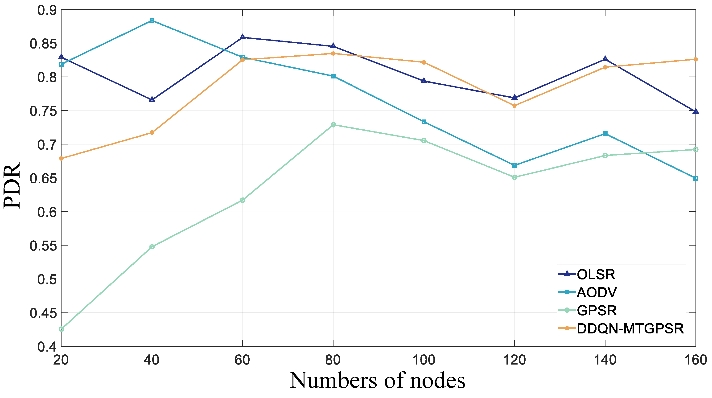
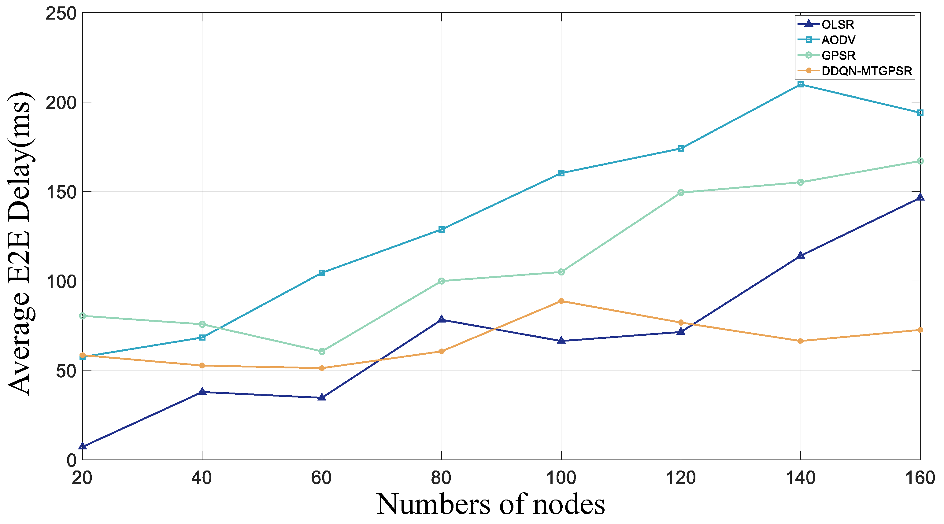
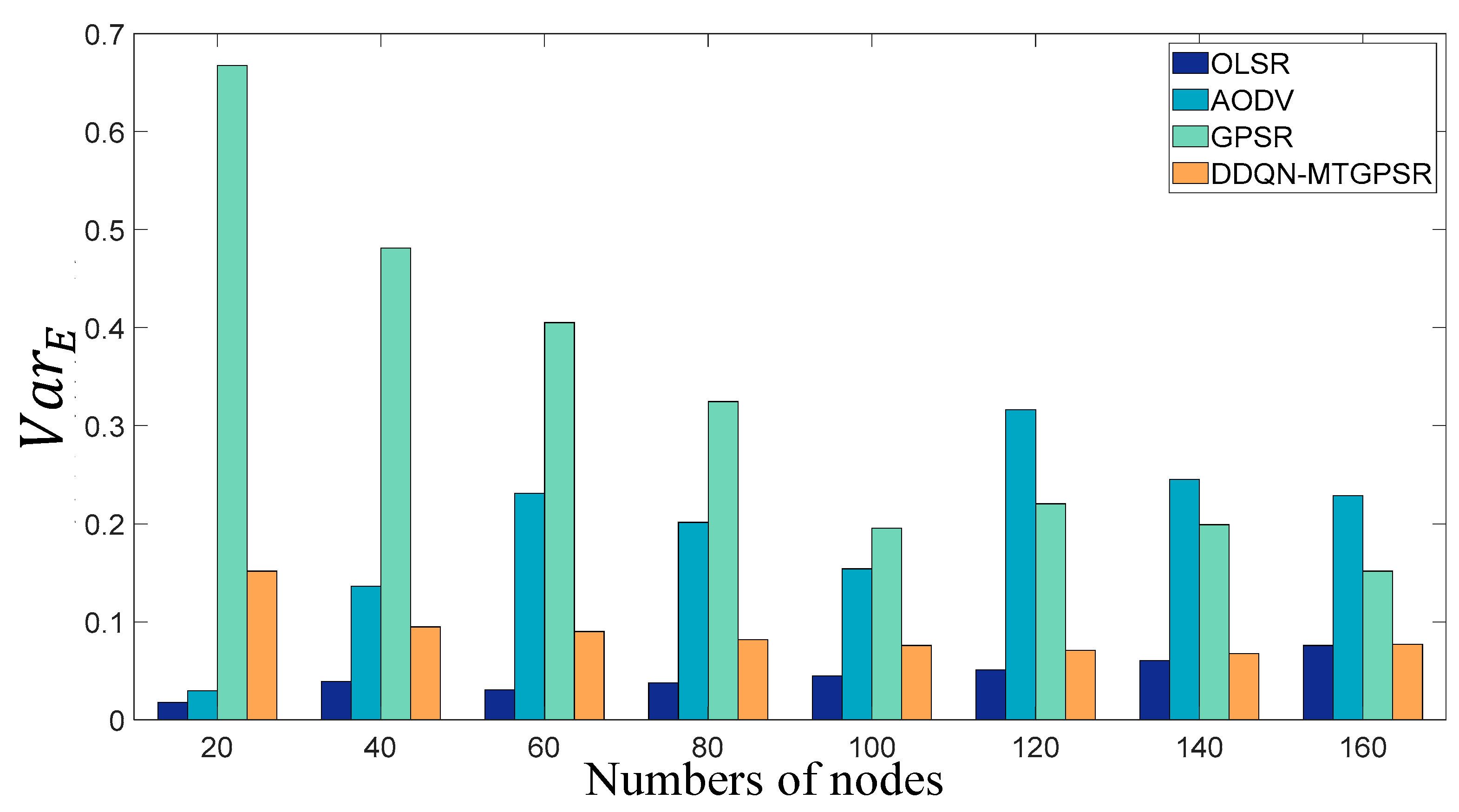
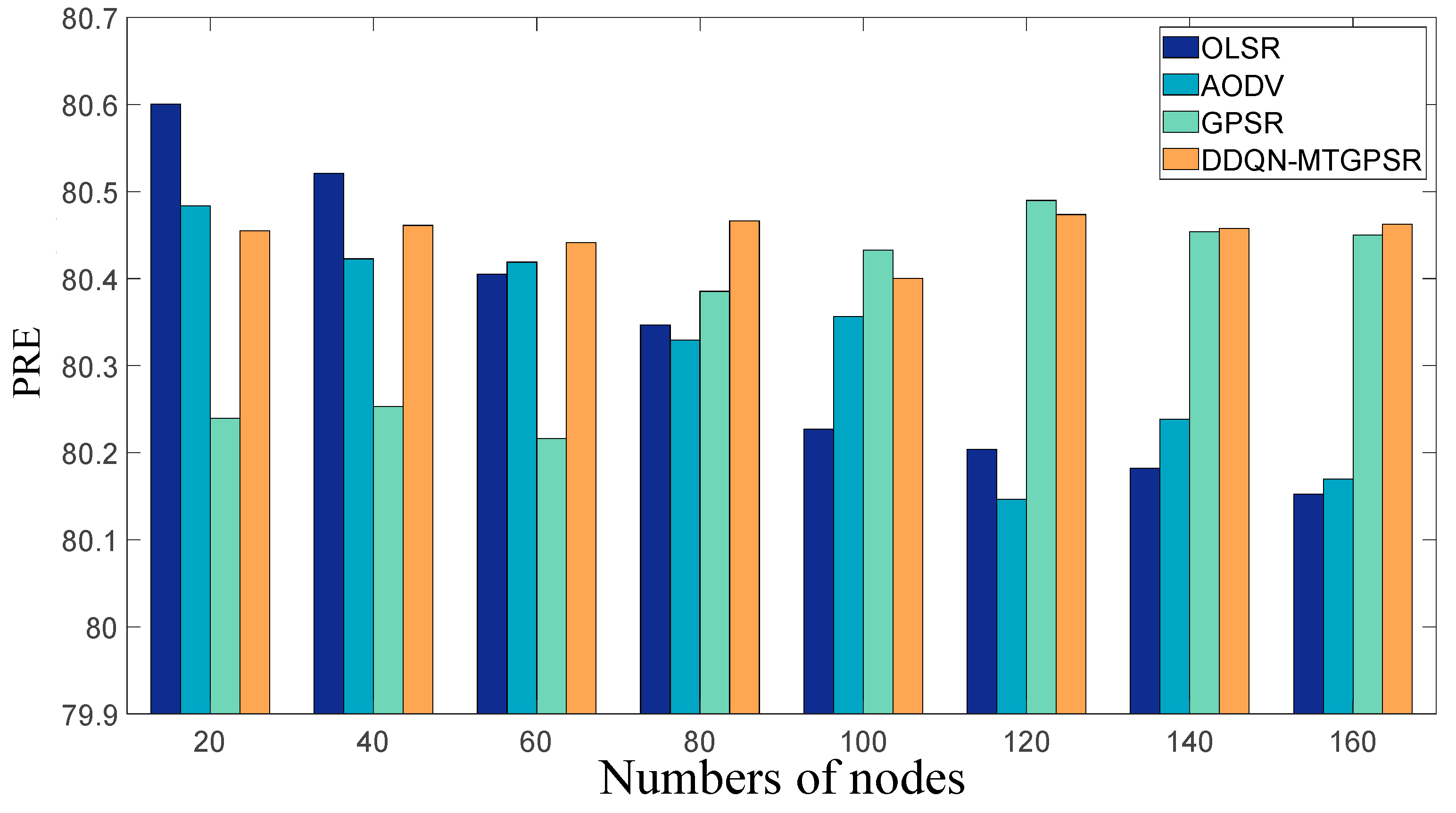
5. Experiments and Analysis of Results

5.1. Simulation Architecture

NS-3 is a network simulator with the advantage of providing full-stack analog simulation from the physical layer to the application layer, but it is unable to implement AI algorithms. Therefore, this study relies on the NS3-AI interface provided by NS-3 to assist the communication between the NS-3 environment and AI framework. The NS3-AI is the NS-3 AI algorithm interface for network research, which is an interaction module between NS-3 and several Python-based AI frameworks, and it can be realized through shared memory for efficient and fast data exchange between the AI algorithms and NS-3 [36]. This module consists of two parts: the NS-3 interface developed in C++ and the AI interface developed in Python. It is the core module for transferring data from one C++ program to another Python program. The NS-3 simulator and the AI framework run in different processes, and data transfer is mainly carried out in two cases: sending NS-3 simulation data to the AI model in Python and testing Python output values in NS-3. The NS-3 simulator is used to establish networks and topological structures and generate simulation data required by artificial intelligence algorithms. The AI framework uses the data in NS-3 to train the model and returns the output of the model to NS-3 for testing. This paper uses the NS3-AI interface and implements DDQN through the AI framework to ensure the continuous interaction between environmental state information and routing decision results during the simulation process.

In NS-3, this study modifies the original GPSR module, extracts the environment state information $s_t$ and inputs it into the shared memory of the NS3-AI interface during the simulation process. Based on the NS3-AI to realize the adaptation of the data structure at both ends, the AI framework PyTorch can immediately obtain the state information from NS-3 through the shared memory, input it into the DDQN, and obtain the routing decision result. The routing decision result is returned to NS-3 through shared memory, and the node forwards the next hop.

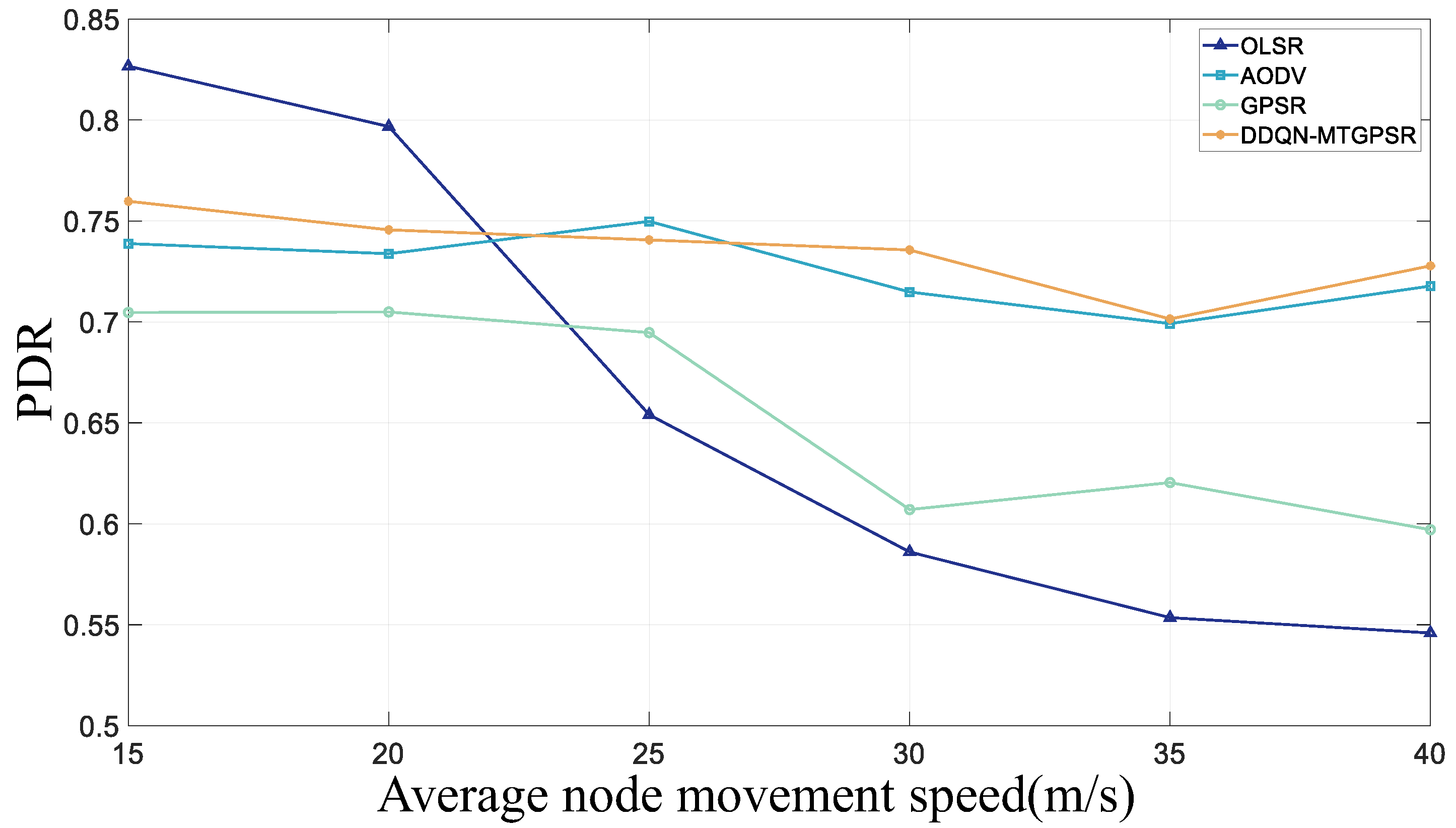
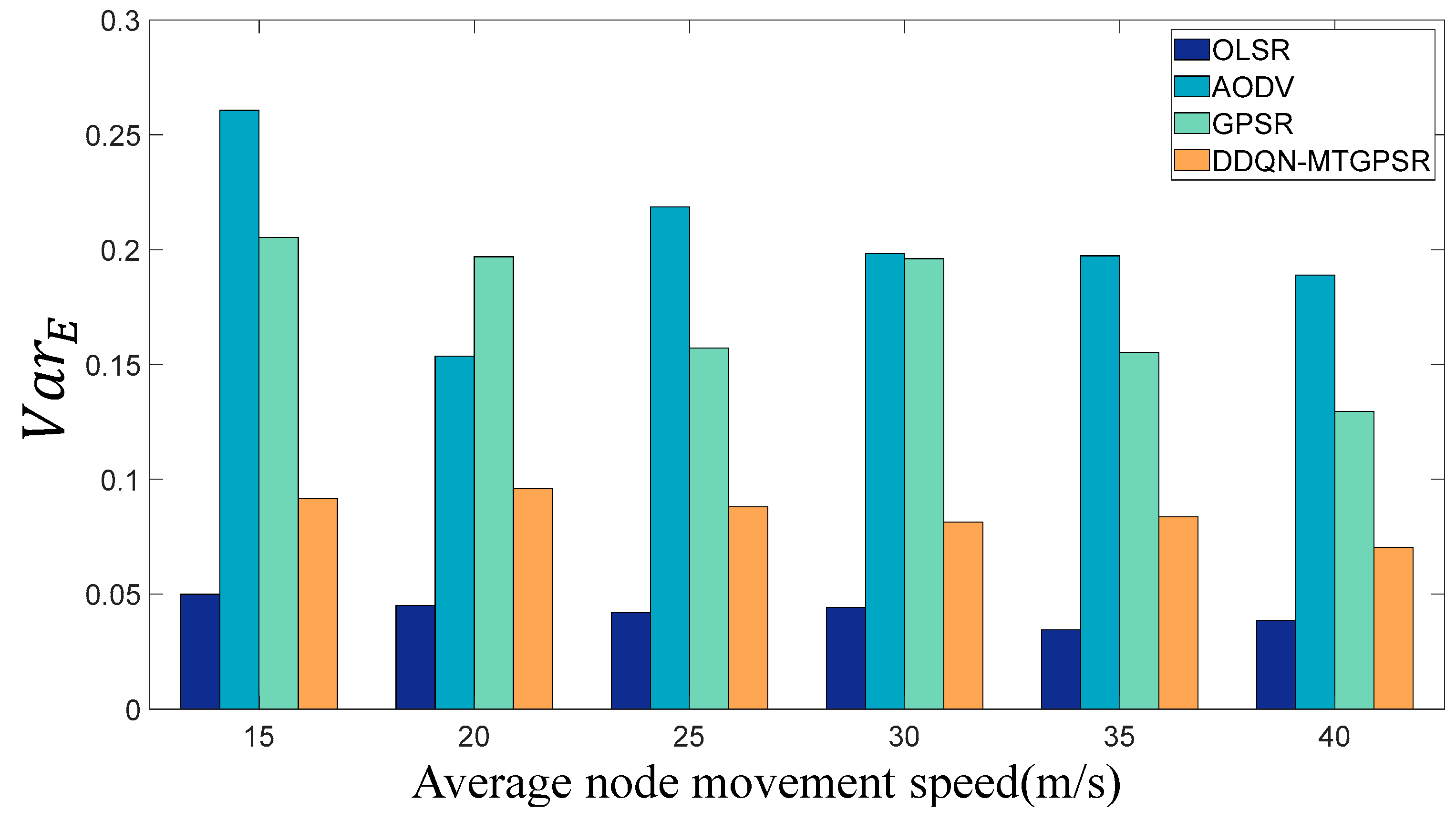
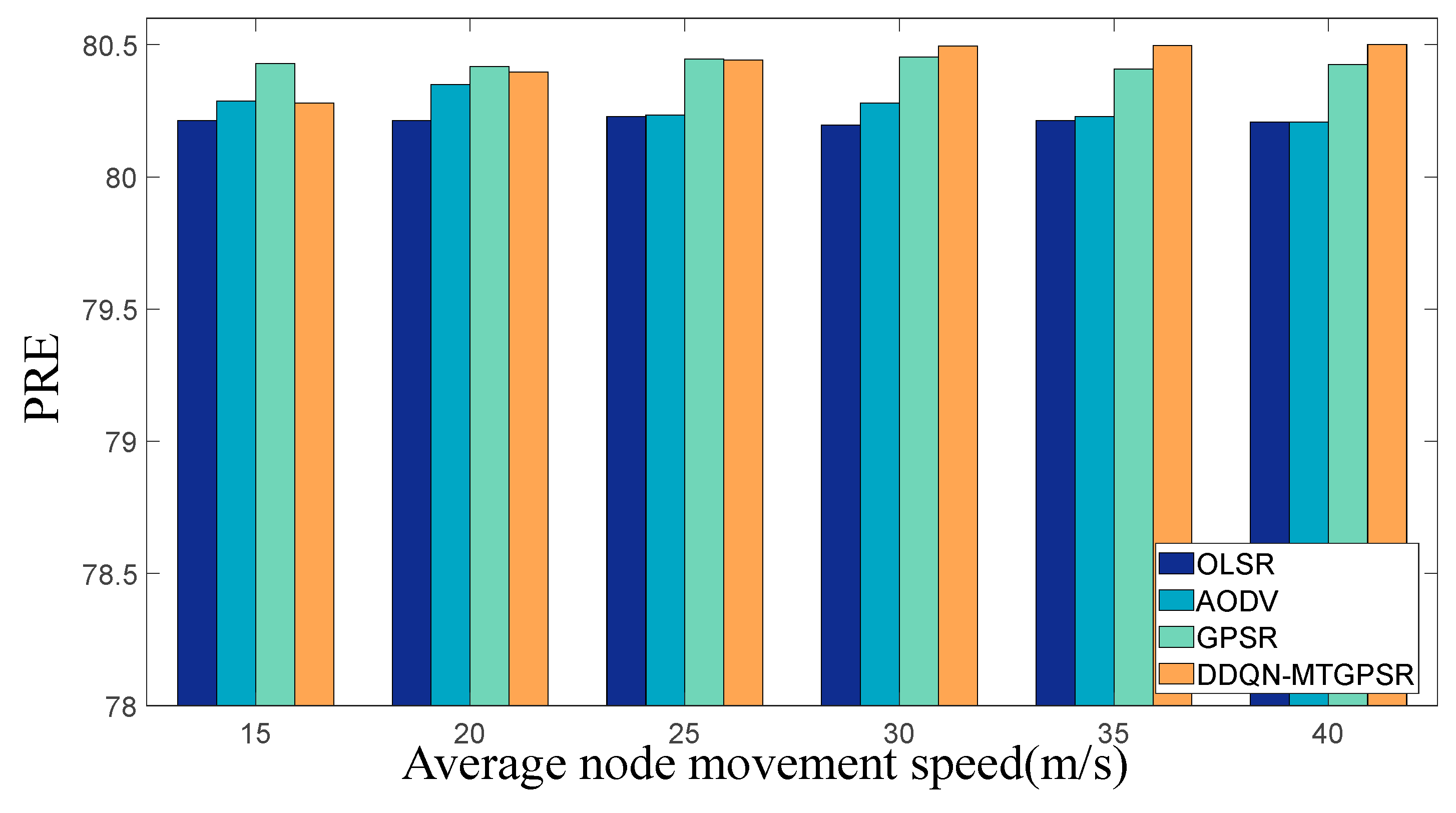
5.2. Experimental Parameters and Results

The experiment sets up 10 nodes that are respectively responsible for sending and receiving services, sending traffic at a constant rate from the beginning of the simulation. Comparison experiments are conducted for the same network scenario to test the performance of different routing protocols in network performance under different network size and mobile speed conditions, respectively. The network performance evaluation metrics are packet delivery rate (PDR), average end-to-end delay (average E2E delay), node average residual energy variance ($Va{r}_E$), and percentage of node average residual energy (PRE). The parameters of the simulation experiment are shown in

Table 4. Table of parameters related to simulation experiments.

Simulation Parameters	Parameter Value
operating system	Ubuntu 20.04
software version	NS-3.30.1
transport layer protocol	UDP
comparative routing protocols	OLSR, AODV, GPSR, DDQN-MTGPSR
MAC/PHY layer protocol	IEEE 802.11b
radiant power	20 dBm
transmission rate	2 Mbps
packet transmission rate	2.048 kb/s
packet length	64 bytes
channel fading model	Friis propagation model
initial energy	300 J
nodal distribution range	$2000 \mathrm{m}\times 2000 \mathrm{m}$
node movement model	randomized waypoint model (RWP)
simulation time	100 s

.

Designing comparative experiments under two different dimensions of average node movement speed and the scale of network, three ad hoc traditional routes with better performance were selected: OLSR [15], AODV [18], and GPSR [21], with the proposed DDQN-MTGPSR algorithm in different scenarios for comparison testing.

(1) Control variable: average speed of node movement.

The effect of different movement speeds on the performance of the routing protocol is tested in NS-3. The initial average mobility speed is set to 15 m/s, incremented to 40 m/s in a gradient of 5, and the total number of nodes is fixed to 100 (moderate network size).

As Figure 3 shows, as the speed of node movement increases, the overall packet delivery rates for several routing protocols show a decreasing trend, albeit to varying extents. The OLSR protocol, which is an active routing protocol that requires regular transmission of control information to maintain the routing table, experiences the most significant decline in packet delivery rates. This is due to the increased frequency of network topology changes with faster movement speeds, which makes OLSR unable to update routing information in time, leading to packet loss. In comparison, AODV, GPSR, and DDQN-MTGPSR show a slower decline in packet delivery rates as the node movement speed increases. Among these, GPSR experiences the lowest packet delivery rates at the same movement speed, while the differences in packet delivery rates between AODV and DDQN-MTGPSR are less pronounced, especially when speed increases. AODV is a demand-driven routing protocol that only establishes routing paths when data forwarding is required, thus ensuring more reliable forwarding paths and maintaining a relatively high level of packet delivery rates. DDQN-MTGPSR algorithm encourages the selection of higher-quality, less congested links, which have a lower likelihood of experiencing holes, thereby reducing the risk of packet loss. Compared to the traditional GPSR, the average packet delivery rate of DDQN-MTGPSR is improved by 12.72%.

As Figure 4 shows, when facing increased node mobility speeds, the Average E2E Delay of OLSR exhibits unstable oscillation behavior with the average node moving speed change. Its proactive management and updating of routing tables lead to frequent adjustments when nodes move at high speeds, necessitating the frequent updating of these tables, which in turn causes significant fluctuations in end-to-end delay. Among all, AODV experiences the highest end-to-end delay under the same conditions of node activity. GPSR and its improved version, DDQN-MTGPSR, exhibit decreasing latencies, mainly due to the on-demand nature of AODV’s routing establishment, which can cause additional delays when the network topology changes rapidly. Traditional GPSR makes routing decisions based on the next hop’s location without going through a full routing discovery process, leading to generally lower delay compared to AODV. The DDQN-MTGPSR algorithm balances multiple routing performance indicators, showcasing a superior end-to-end delay compared to GPSR and AODV, especially under certain node mobility speeds, approaching the OLSR performance. In comparison to traditional GPSR, the end-to-end delay of DDQN-MTGPSR is, on average, reduced by 20.05%.

As Figure 5 shows, the increase in $Va{r}_E$, due to node movement speed, when using OLSR with DDQN-MTGPSR, is not notably significant. OLSR boasts an active routing and multi-point forwarding mechanism, which distributes network control messages and energy consumption evenly across nodes. Even as the speed of nodes increases, the energy consumption per node stays relatively consistent, rendering the variance in energy consumption insensitive to velocity changes. DDQN-MTGPSR incorporates the remaining energy level of neighboring nodes, prioritizing the selection of nodes with higher remaining energy for forwarding, thus helping to balance energy consumption among nodes. Despite DDQN-MTGPSR’s introduction of link quality and routing hole, which enhances the connectivity, it still operates based on local topologies, leading to slightly higher variance compared to OLSR. Comparatively, AODV and GPSR display consistently higher variances. AODV is an on-demand routing protocol, and GPSR relies on local information of one-hop neighbor locations, neither of which can meticulously obtain the entire network topology or achieve an even distribution of energy usage. This can lead to some nodes shouldering more of the routing discovery and data forwarding tasks, contributing to an uneven distribution of energy consumption. However, GPSR exhibits lower variance than AODV thanks to its location-aware routing strategy, which more efficiently adapts to topological changes when dealing with rapidly moving nodes. It quickly directs attention to the next hop closer to the destination, avoiding the additional energy expenditure that arises from searching for new routes, a characteristic that AODV frequently engages in during these scenarios. The average residual energy variance of nodes for DDQN-MTGPSR is reduced by 50.15% on average as compared to GPSR.

As Figure 6 shows, when the speed is low because GPSR does not need to maintain a complex routing table, it maintains a higher PRE. In a highly dynamic network, AODV requires frequent route discovery, and OLSR needs to continuously update routing information so the remaining energy is lower than that of GPSR. Under low-speed conditions, the topology changes are not too frequent. Although DDQN-GPSR introduces various environmental states to improve network performance, at the same time, its broadcast packets have been changed, and the fields are longer, so the overhead is slightly higher than that of GPSR. However, at high speeds, GPSR incurs increased overhead due to frequent switching to the recovery mode, while DDQN-GPSR has more selectable neighbors and higher routing efficiency, thereby reducing the overall overhead compared to GPSR. Compared to GPSR, the PRE of DDQN-MTGPSR has increased by an average of 0.47%.

In summary, compared with GPSR, the DDQN-GPSR routing protocol comprehensively improves various indicators. At the same time, the experimental results show that OLSR and AODV are not suitable for extremely high-speed scenarios, and the packet delivery rate of the former and the delay of the latter are prone to negative performance due to the change in moving speed. DDQN-MTGPSR is less susceptible to speed changes than the first two. The delivery rate and delay combination prove that DDQN-MTGPSR is more suitable for high-dynamic scenarios than OLSR and AODV. In addition, the ratio of residual energy between OLSR and AODV is lower than that of DDQN-MTGPSR in high-speed scenarios. From the perspective of residual energy variance, DDQN-MTGPSR can still balance the energy consumption of each node as much as possible in high-speed scenarios, which is better than AODV but slightly worse than OLSR. However, from the perspective of comprehensive communication quality performance, it can still be concluded that DDQN-MTGPSR is more suitable for highly dynamic UAV cluster networks.

(2) Control variable: scale of network.

To test the effect of different scales of the network on routing performance in the same area, the total number of initial nodes was set to 20 and gradually increased to 160 at intervals of 20 nodes, with an average movement speed of 20 m/s for each node.

As Figure 7 shows, as the number of nodes in the network increases, the packet delivery rates of both GPSR and DDQN-MTGPSR show an increasing trend. OLSR, on the other hand, tends to exhibit fluctuations within a certain range, while AODV follows an overall decreasing trend. GPSR is more sensitive to density, meaning the greater the number of nodes in the network, the more options there are for GPSR to select as neighboring nodes, thus leading to a higher packet delivery rate. As the number of nodes grows, the network topology becomes more complex, which presents a challenge for timely updates of routing information in OLSR. This can result in some nodes experiencing delays, thus causing fluctuations in the packet delivery rate. With an increase in the number of nodes, the process of establishing routes in AODV becomes more intricate, leading to increased data packet dropouts. For DDQN-GPSR, when the number of nodes is relatively small, its packet delivery rate is indeed lower compared to OLSR and AODV. However, it surpasses GPSR, mainly because of the incorporation of additional state features. Even though DDQN-GPSR still operates as a local topology-based routing protocol, it exhibits significantly reduced packet loss. As the network contains more nodes, the packet delivery rate of DDQN-GPSR tends to remain at a relatively high level, and in certain scenarios, it can match or even surpass OLSR’s delivery rate while still outperforming AODV. Compared to GPSR, the PDR of DDQN-MTGPSR is found to be 26.26% higher.

AS Figure 8 shows, as the number of nodes increases, the average E2E delay of GPSR decreases first and then increases. This is because increasing the number can increase the number of optional neighbors, which helps to reduce the delay. However, if the nodes become more dense, routing loops and routing holes will cause the delay to increase. The delay of AODV and OLSR increases significantly. AODV establishes routes on demand. The increase in network density leads to longer route establishment time. The rapid increase in the number of OLSR-controlled messages will cause network congestion and increase the delay. The average E2E delay of DDQN-MTGPSR is less affected by the change in the scale of the network and can fluctuate in a relatively low range. Due to the introduction of other routing performance indicators, the algorithm is prompted to select paths with less congestion, more reliable links, and fewer routing holes, reducing the end-to-end delay to a certain extent. Compared to GPSR, the end-to-end delay of DDQN-MTGPSR is reduced by 36.31% on average.

As Figure 9 shows, AODV’s $Va{r}_E$ exhibits a significant elevation as the number of nodes increases and fluctuates within a relatively high range. When the number of nodes is very small, the GPSR protocol exhibits a very high $Va{r}_E$, and as the number of nodes increases, the number of neighbors available for GPSR to choose from increases, and the energy consumption becomes more uniform. The $Va{r}_E$ of OLSR is maintained at a relatively low level but shows an overall increasing trend. DDQN-MTGPSR introduces the residual energy of the neighboring nodes, and DDQN-MTGPSR is able to prioritize forwarding nodes with higher residual energy, which plays a role in balancing the energy consumption among nodes, so $Va{r}_E$ is lower under large-scale networks. Nodes' average residual energy variance is reduced by 69.3% on average in DDQN-MTGPSR compared to GPSR.

As shown in Figure 10, the more nodes in the network, the more control messages need to be transmitted and processed, so the PRE of OLSR continues to decline. AODV shows a downward trend as a whole. The more nodes, the more complicated the route establishment process of AODV and the more energy consumed. The GPSR protocol is more sensitive to the density of the node. It can be used with fewer neighbors with extremely low density. It may trigger extremely frequent peripheral repost mode, so the routing efficiency is low. As the density of the node increases, this situation has improved, and the surplus energy proportion of GPSR networks is higher than that of AODV and OLSR. Because the DDQN-MTGPSR has a longer radio signal field, compared to GPSR’s control overhead, but due to the introduction of other routing performance indicators, the routing efficiency of DDQN-MTGPSR is higher, and its overall expenses will not be significantly higher than that GPSR has the phenomenon of ups and downs fluctuations between the two. Compared with GPSR, the surplus energy of DDQN-MTGPSR has increased by 8.709% on average.

Compared with GPSR, with the increase of network scale, DDQN-MTGPSR basically has a comprehensive improvement on the evaluation indicators. Based on all evaluation indicators to analyze, OLSR and AODV are not suitable for large-scale scenarios. The extension of the former’s end-to-end is significantly increased with the increase in the number of nodes. Regarding the trend of decline and increase, unlike OLSR and AODV, the increase in network scale will not have a significant negative effect on the performance of DDQN-MTGPSR in terms of delay and delivery rate. In large-scale scenarios, its delivery rate is higher than AODV and close to OLSR. The delay can be lower than AODV and lower than OLSR under certain high-density conditions. In addition, the surplus energy of OLSR and AODV will gradually be lower than the DDQN-MTGPSR with the increase in nodes. From the perspective of the remaining energy difference, the DDQN-MTGPSR is better than AODV due to the increase in the number of nodes and can be close to OLSR, indicating that DDQN-MTGPSR can balance the energy consumption of each node in large-scale networks. In summary, DDQN-MTGPSR is suitable for large-scale UAV cluster networks.

Combining all the experimental results under the two experimental conditions and considering the comprehensive performance of the network, including communication quality of service and energy consumption, DDQN-MTGPSR is more suitable for large-scale and highly dynamic UAV clusters than the other three routing protocols.

6. Conclusions

In this study, we focus on the environmental characteristics of UAV clusters and aim to develop an intelligent routing protocol that adapts to highly dynamic and large-scale networks. We have designed a multi-objective optimized GPSR routing protocol based on DDQN (DDQN-MTGPSR).

Firstly, we addressed the mathematical modeling of the multi-objective routing optimization problem by integrating the multi-objective optimization mechanism of DDQN. The route forwarding process is transformed into a Markov decision process (MDP), and we achieve the modeling of the multi-objective routing optimization problem by comprehensively considering various routing performance indicators through a mixed-objective approach. Subsequently, based on the mathematical modeling of the routing problem, we employed the DDQN algorithm to improve the traditional route forwarding mechanism of GPSR and constructed a DDQN model tailored to solve the routing problem in this study. Finally, to evaluate the performance of the proposed algorithm, we integrated the NS-3 network simulator with an AI framework using the NS3-AI interface. This integration allowed us to implement the DDQN-MTGPSR intelligent routing protocol and verify its advantages through simulation experiments. The results demonstrate that DDQN-MTGPSR outperforms comparative routing protocols in large-scale and highly dynamic networks.

Although this study has made some progress in optimizing routing protocols for UAV clusters, some important research issues still need to be further explored. Firstly, the broadcast beacons in DDQN-MTGPSR include additional fields beyond traditional GPSR location information, leading to increased control overhead compared to conventional GPSR routing protocols. Additionally, the exploration–exploitation balance mechanism employs a fixed exploration rate (ε), which may not be optimal for all network conditions.

Future work will focus on introducing an adaptive HELLO message mechanism to reduce control overhead by minimizing the frequency of control information transmissions. To enhance algorithm performance, we plan to design an adaptive ε based on time or network stability, reducing unnecessary exploration under stable conditions to improve convergence and routing efficiency. In addition, as the scale of UAV clusters continues to expand and the application scenarios become more complex, dynamic management of nodes will become one of the key challenges. Future work can explore how to better cope with network topology changes caused by nodes' addition or exit. Introducing more flexible and adaptive mechanisms can better support the practical application of UAV clusters in complex and dynamic environments.

References

1. Niyazi, M.; Behnamian, J. Application of Emerging Digital Technologies in Disaster Relief Operations: A Systematic Review. Arch. Comput. Methods Eng. 2023, 30, 1579–1599. [Google Scholar] [CrossRef]
2. Flakus, J. Use of Large Unmanned Vehicles in Joint Intelligence, Surveillance, and Reconnaissance. Available online: https://apps.dtic.mil/sti/trecms/pdf/AD1174711.pdf (accessed on 27 June 2024).
3. Loukinas, P. Drones for Border Surveillance: Multipurpose Use, Uncertainty and Challenges at EU Borders. Geopolitics 2022, 27, 89–112. [Google Scholar] [CrossRef]
4. Xu, G.; Jiang, W.; Wang, Z.; Wang, Y. Autonomous Obstacle Avoidance and Target Tracking of UAV Based on Deep Reinforcement Learning. J. Intell. Robot. Syst. 2022, 104, 60. [Google Scholar] [CrossRef]
5. Liang, Z.; Li, Q.; Fu, G. Multi-UAV Collaborative Search and Attack Mission Decision-Making in Unknown Environments. Sensors 2023, 23, 7398. [Google Scholar] [CrossRef] [PubMed]
6. Shahzadi, R.; Ali, M.; Naeem, M. UAV Placement and Resource Management in Public Safety Networks: An Overview. In Intelligent Unmanned Air Vehicles Communications for Public Safety Networks; Kaleem, Z., Ahmad, I., Duong, T.Q., Eds.; Unmanned System Technologies; Springer Nature: Singapore, 2022; pp. 19–49. ISBN 978-981-19129-2-4. [Google Scholar]
7. AL-Dosari, K.; Hunaiti, Z.; Balachandran, W. Systematic Review on Civilian Drones in Safety and Security Applications. Drones 2023, 7, 210. [Google Scholar] [CrossRef]
8. Cheng, L.; Tan, X.; Yao, D.; Xu, W.; Wu, H.; Chen, Y. A Fishery Water Quality Monitoring and Prediction Evaluation System for Floating UAV Based on Time Series. Sensors 2021, 21, 4451. [Google Scholar] [CrossRef] [PubMed]
9. Aissaoui, R.; Deneuville, J.-C.; Guerber, C.; Pirovano, A. A Survey on Cryptographic Methods to Secure Communications for UAV Traffic Management. Veh. Commun. 2023, 44, 100661. [Google Scholar] [CrossRef]
10. Ding, R.; Chen, J.; Wu, W.; Liu, J.; Gao, F.; Shen, X. Packet Routing in Dynamic Multi-Hop UAV Relay Network: A Multi-Agent Learning Approach. IEEE Trans. Veh. Technol. 2022, 71, 10059–10072. [Google Scholar] [CrossRef]
11. Arafat, M.Y.; Moh, S. Routing Protocols for Unmanned Aerial Vehicle Networks: A Survey. IEEE Access 2019, 7, 99694–99720. [Google Scholar] [CrossRef]
12. Peng, J.-X.; Yuan, L.-F.; Liu, S.; Zhang, Q. Review of Unmanned Cluster Routing Protocols Based on Deep Reinforcement Learning. In Proceedings of the International Conference on Signal Processing and Communication Technology (SPCT 2022), Harbin, China, 6 April 2023; Volume 12615, pp. 572–579. [Google Scholar]
13. Peng, H.; Razi, A.; Afghah, F.; Ashdown, J. A Unified Framework for Joint Mobility Prediction and Object Profiling of Drones in UAV Networks. J. Commun. Netw. 2018, 20, 434–442. [Google Scholar] [CrossRef]
14. Perkins, C.E.; Bhagwat, P. Highly Dynamic Destination-Sequenced Distance-Vector Routing (DSDV) for Mobile Computers. SIGCOMM Comput. Commun. Rev. 1994, 24, 234–244. [Google Scholar] [CrossRef]
15. Jacquet, P.; Muhlethaler, P.; Clausen, T.; Laouiti, A.; Qayyum, A.; Viennot, L. Optimized Link State Routing Protocol for Ad Hoc Networks. In Proceedings of the IEEE International Multi Topic Conference, 2001. IEEE INMIC 2001. Technology for the 21st Century, Lahore, Pakistan, 30 December 2001; pp. 62–68. [Google Scholar]
16. Arafat, M.Y.; Moh, S. A Q-Learning-Based Topology-Aware Routing Protocol for Flying Ad Hoc Networks. IEEE Internet Things J. 2022, 9, 1985–2000. [Google Scholar] [CrossRef]
17. Johnson, D.B.; Maltz, D.A.; Broch, J. DSR: The Dynamic Source Routing Protocol for Multi-Hop Wireless Ad Hoc Networks. Ad. Hoc Netw. 2001, 5, 139–172. [Google Scholar]
18. Chakeres, I.D.; Belding-Royer, E.M. AODV Routing Protocol Implementation Design. In Proceedings of the 24th International Conference on Distributed Computing Systems Workshops, Tokyo, Japan, 23–24 March 2004; pp. 698–703. [Google Scholar]
19. Rovira-Sugranes, A.; Razi, A.; Afghah, F.; Chakareski, J. A Review of AI-Enabled Routing Protocols for UAV Networks: Trends, Challenges, and Future Outlook. Ad. Hoc Netw. 2022, 130, 102790. [Google Scholar] [CrossRef]
20. Arafat, M.Y.; Moh, S. Bio-Inspired Approaches for Energy-Efficient Localization and Clustering in UAV Networks for Monitoring Wildfires in Remote Areas. IEEE Access 2021, 9, 18649–18669. [Google Scholar] [CrossRef]
21. Karp, B.; Kung, H.T. GPSR: Greedy Perimeter Stateless Routing for Wireless Networks. In Proceedings of the 6th Annual International Conference on Mobile Computing and Networking, Boston, MA, USA, 6–11 August 2000; Association for Computing Machinery: New York, NY, USA, 1 August, 2000; pp. 243–254. [Google Scholar]
22. Boyan, J.; Littman, M. Packet Routing in Dynamically Changing Networks: A Reinforcement Learning Approach. Adv. Neural Inf. Process. Syst. 1993, 6, 671–678. [Google Scholar]
23. Jung, W.-S.; Yim, J.; Ko, Y.-B. QGeo: Q-Learning-Based Geographic Ad Hoc Networks. IEEE Commun. Lett. 2017, 21, 2258–2261. [Google Scholar] [CrossRef]
24. Jin, W.; Gu, R.; Ji, Y. Reward Function Learning for Q-Learning-Based Geographic Routing Protocol. IEEE Commun. Lett. 2019, 23, 1236–1239. [Google Scholar] [CrossRef]
25. Park, C.; Lee, S.; Joo, H.; Kim, H. Empowering Adaptive Geolocation-Based Routing for UAV Networks with Reinforcement Learning. Drones 2023, 7, 387. [Google Scholar] [CrossRef]
26. Rao, Z.; Xu, Y.; Pan, S. A Deep Learning-Based Constrained Intelligent Routing Method. Peer-to-Peer Netw. Appl. 2021, 14, 2224–2235. [Google Scholar] [CrossRef]
27. Liu, D.; Zhang, J.; Cui, J.; Ng, S.-X.; Maunder, R.G.; Hanzo, L. Deep-Learning-Aided Packet Routing in Aeronautical Ad Hoc Networks Relying on Real Flight Data: From Single-Objective to Near-Pareto Multiobjective Optimization. IEEE Internet Things J. 2022, 9, 4598–4614. [Google Scholar] [CrossRef]
28. Gurumekala, T.; Indira Gandhi, S. Toward In-Flight Wi-Fi: A Neuro-Fuzzy Based Routing Approach for Civil Aeronautical Ad Hoc Network. Soft Comput. 2022, 26, 7401–7422. [Google Scholar] [CrossRef]
29. Ryu, K.; Kim, W. Multi-Objective Optimization of Energy Saving and Throughput in Heterogeneous Networks Using Deep Reinforcement Learning. Sensors 2021, 21, 7925. [Google Scholar] [CrossRef]
30. Moon, S.; Koo, S.; Lim, Y.; Joo, H. Routing Control Optimization for Autonomous Vehicles in Mixed Traffic Flow Based on Deep Reinforcement Learning. Appl. Sci. 2024, 14, 2214. [Google Scholar] [CrossRef]
31. Yu, S.; Dingcheng, D. Multi-Objective Mission Planning for UAV Swarm Based on Deep Reinforcement Learning. In Proceedings of the 2023 IEEE International Conference on Unmanned Systems (ICUS), Hefei, China, 13–15 October 2023; pp. 1–10. [Google Scholar]
32. Lacage, M.; Henderson, T.R. Yet Another Network Simulator. In Proceedings of the 2006 Workshop on Ns-3, Pisa, Italy, 10 October 2006; Association for Computing Machinery: New York, NY, USA, 2006; p. 12–es. [Google Scholar]
33. Lyu, N.; Song, G.; Yang, B.; Cheng, Y. QNGPSR: A Q-Network Enhanced Geographic Ad-Hoc Routing Protocol Based on GPSR. In Proceedings of the 2018 IEEE 88th Vehicular Technology Conference (VTC-Fall), Chicago, IL, USA, 27–30 August 2018; pp. 1–6. [Google Scholar]
34. Lansky, J.; Rahmani, A.M.; Hosseinzadeh, M. Reinforcement Learning-Based Routing Protocols in Vehicular Ad Hoc Networks for Intelligent Transport System (ITS): A Survey. Mathematics 2022, 10, 4673. [Google Scholar] [CrossRef]
35. Liu, J.; Wang, Q.; He, C.; Jaffrès-Runser, K.; Xu, Y.; Li, Z.; Xu, Y. QMR:Q-Learning Based Multi-Objective Optimization Routing Protocol for Flying Ad Hoc Networks. Comput. Commun. 2020, 150, 304–316. [Google Scholar] [CrossRef]
36. Yin, H.; Liu, P.; Liu, K.; Cao, L.; Zhang, L.; Gao, Y.; Hei, X. Ns3-Ai: Fostering Artificial Intelligence Algorithms for Networking Research. In Proceedings of the 2020 Workshop on ns-3, Gaithersburg, MD, USA, 17–18 June 2020; pp. 57–64. [Google Scholar] [CrossRef]
Figure 1. Routing hole avoidance for neighboring nodes.
Mathematics 12 02672 g001
Figure 2. DDQN model interacting with the network environment.
Mathematics 12 02672 g002
Figure 3. Variation of PDR with average speed.
Mathematics 12 02672 g003
Figure 4. Variation of average E2E delay with average speed.
Mathematics 12 02672 g004
Figure 5. Variation of V a r E with the average speed.
Mathematics 12 02672 g005
Figure 6. Variation of PRE with average speed.
Mathematics 12 02672 g006
Figure 7. Variation of PDR with the scale of the network.
Mathematics 12 02672 g007
Figure 8. Variation of average E2E delay with the scale of the network.
Mathematics 12 02672 g008
Figure 9. Variation of V a r E with the scale of the network.
Mathematics 12 02672 g009
Figure 10. Variation of PRE with the scale of the network.
Mathematics 12 02672 g010