A Two-Echelon Routing Model for Sustainable Last-Mile Delivery with an Intermediate Facility: A Case Study of Pharmaceutical Distribution in Rome

Abstract

This paper introduces a two-echelon optimization model for the integrated routing of an electric vehicle (EV) and a traditional internal combustion engine vehicle (ICEV) in an urban environment. The scientific context of this study is sustainable urban logistics. The case study focuses on the distribution of pharmaceuticals in the metropolitan area of Rome. Distributing pharmaceuticals in large cities presents significant challenges, including heavy traffic congestion, the need for strict temperature control, and the maintenance of the integrity and timely delivery of sensitive medications. Furthermore, the complexity of urban logistics and adherence to regulatory requirements introduce additional layers of difficulty. Therefore, the implementation of fast and sustainable distribution mechanisms is crucial in this context. Specifically, the model seeks to minimize both total CO₂ emissions and transportation costs while optimizing the use of an EV and an ICEV, all while ensuring that service level requirements are met. Computational results demonstrate the effectiveness of the proposed method in improving the sustainability of pharmaceutical distribution.

1. Introduction

Urban logistics, particularly in the context of sustainable city logistics, faces significant challenges due to the increasing demand for delivery services, traffic congestion, and environmental concerns. The urgent need for a sustainable transition in the logistics sector amplifies these challenges. Last-mile logistics is pivotal in this direction, with requests for last-mile delivery expected to grow by up to 78% by 2030 [1]. The discussion on the Sustainable Development Goals (SDGs) introduced by the United Nations 2030 Agenda [2] has spurred numerous green logistics initiatives. These initiatives have the potential to decrease air pollution and mitigate negative health impacts (good health and well-being SDG), as well as play a crucial role in climate resilience (climate action SDG).

To mitigate the impacts of last-mile logistics, several significant innovations have been introduced over the past decade. These innovations leverage new information and communication technologies [3,4], electric and clean vehicles [5], and collaborative approaches [6]. They have the potential to enhance efficiency and reduce logistics costs (economic growth SDG), improve intermodal exchanges (industry, innovation, and infrastructure SDG), and optimize vehicle routing (sustainable cities and communities SDG).

Integrating electric vehicles (EVs) into urban delivery fleets offers a promising solution to mitigate environmental impacts and enhance the efficiency of logistics operations [7]. This paper introduces an optimization model for the combined routing of an EV and a traditional internal combustion engine vehicle (ICEV) for the distribution of pharmaceuticals in Rome considering an intermediate facility.

The pharmaceutical distribution sector is critically dependent on timely and efficient delivery services, making it an ideal candidate for exploring the benefits of sustainable logistics solutions [8,9,10]. This paper addresses this challenge by analyzing the benefits and costs of using a mixed fleet within a dense urban area for pharmaceutical distribution.

In Italy, the distribution of medicines to pharmacies follows a well-organized operational process. Pharmaceuticals are typically stored in large, centralized warehouses managed by pharmaceutical wholesalers. Orders from pharmacies are collected via electronic systems, which streamline the process and ensure accuracy. Once an order is received, the medicines are picked, packed, and prepared for shipment within the warehouse. The goods are then loaded onto temperature-controlled delivery vans to maintain the integrity of the pharmaceuticals during transport. These vehicles follow pre-planned routes that optimize delivery efficiency, often utilizing regional distribution centers (RDCs) for further coordination. Deliveries are usually scheduled to ensure that RDCs receive their stock promptly, often within 24 to 48 h.

In the last mile, pharmacies place orders directly with wholesalers very frequently, up to four times a day. Pharmacies expect wholesalers to deliver medicines within 4 to 12 h. It is worth noting that in Italy, pharmacies hold significant contractual power over wholesalers. This means that within the urban area, deliveries to pharmacies can occur on average twice a day. Upon arrival at the pharmacy, the delivery is checked against the order, and any discrepancies are addressed immediately to ensure that pharmacies can meet the needs of their customers without interruption [11].

This work was inspired by the challenge of solving a distribution problem posed by a private company which operates as a logistics service provider (LSP) responsible for distributing medicines in the city of Rome. The company, which initially conducted deliveries using ICEV-type vehicles, has decided to modernize part of its fleet by introducing EVs. This decision is in line with the evolving requirements for distribution in large cities, where commercial vehicles with lower fuel efficiency are gradually being banned from central urban areas. As a result, the LSP’s distribution strategy must be reorganized, with the primary objective of minimizing CO₂ emissions.

The remainder of the paper is organized as follows: Section 1.1 introduces the real-world context provided by the company; Section 2.1 presents the literature review; Section 2.3 details the mathematical formulation; Section 3.1 offers a comprehensive description of the case study; Section 3.2 and Section 3.3 discuss the experimental analysis; and Section 4 concludes with final remarks and future perspectives.

1.1. Context Description

The LSP in question distributes pharmaceutical products within the city twice daily. Each vehicle starts its scheduled delivery route at 8:00 a.m. and 3:00 p.m., respectively. This schedule ensures that pharmacies receive morning deliveries for orders placed by 9:00 p.m. the previous day and afternoon deliveries for orders placed by 1:00 p.m. the same day. It is important to note that this delivery scheme applies to regular distribution, while emergency deliveries are managed separately.

Considering the high number of pharmacies operating in the city, more than 750, the distribution of medicines is organized by dividing the city into several zones and clustering customers based on geographical areas, with each zone associated with a different depot (sometimes shared between zones). The advantages of a zone-based distribution scheme in complex delivery problems are discussed in Bertazzi et al. [12] and Beraldi et al. [13]. The number of zones is sufficiently large to allow each one to be served by a single route. In fact, based on the available historical data, each delivery route takes no more than six hours.

Under these conditions, each vehicle can return to the depot after the first route to load products for the second delivery tour. For the transportation of medicines, the LSP uses packaging boxes with dimensions of (30 × 20 × 15) cm³ or (40 × 30 × 20) cm³, delivering one or two boxes to each pharmacy per tour.

The LSP currently employs a fleet of temperature-controlled ICEVs for deliveries, each with a capacity of approximately 10 m³, capable of accommodating packaging boxes for up to 100 pharmacies simultaneously, if necessary.

To modernize its fleet and reduce the environmental impact of deliveries, the company purchases a series of temperature-controlled EVs to replace some of its older ICEVs, particularly those associated with higher pollution classes that are no longer permitted to operate within the city center of Rome.

From this perspective, the company plans to organize deliveries in each zone using two vehicles: a temperature-controlled EV and a temperature-controlled ICEV. Each EV can be stationed at an intermediate facility, located near a pharmacy, where there is a charging station. The LSP must decide which pharmacies to serve with the EV and which to serve with the ICEV within each zone, while also ensuring that the intermediate facility is visited for crossdocking. The company’s primary goal is to plan routes that minimize environmental emissions and transportation costs while maintaining an appropriate balance in the number of deliveries assigned to each vehicle, without compromising service speed and efficiency (and potentially even improving them). This approach aims to enhance overall fleet management while adhering to more sustainable practices.

The delivery scheme for each zone is described in Figure 1. Note that the zones defined by the LSP are intentionally small (each one covering only a few city districts) to allow vehicles completion of each delivery round within a few hours. Additionally, the EV has time to recharge at the depot during idle hours. As observed by the historical data, this distribution method ensures that driver shift time limits and vehicle capacity constraints are satisfied. All numerical details of the case study are described in Section 3.1.

Given the real-world context, the contribution of this work can be summarized as follows:

• defining and formulating a two-echelon bi-objective routing problem with an intermediate facility to establish the delivery scheme within each urban zone with the aim of planning sustainable and cost-effective routes;
• solving the problem and conducting a what-if analysis based on the available data, assessing the benefits and drawbacks of this delivery scheme and the use of a mixed fleet.

By leveraging the unique advantages of EVs, such as lower emissions and reduced operational costs due to the ability to access low-emission zones in cities, alongside the flexibility and longer range of ICEVs, the proposed model aims to enhance the overall efficiency and sustainability of urban logistics operations.

2. Materials and Methods

2.1. Literature Review

The integration of EVs into logistics operations has been extensively studied, with a focus on their potential to reduce greenhouse gas emissions and operational costs. Previous research has highlighted the challenges associated with the limited range and longer charging times of EVs, necessitating the development of sophisticated optimization models to effectively utilize these vehicles in urban logistics [14,15].

Several studies have explored the vehicle routing problem (VRP) for mixed fleets, incorporating both EVs and traditional vehicles. These models typically aim to minimize operational costs, considering factors such as vehicle range, charging infrastructure, and environmental impact. For an excellent overview of these problems, readers can refer to the surveys by Kucukoglu et al. [7] and Tomislav et al. [16].

One of the most popular applications of these elements is the city logistics framework for last-mile delivery. In this context, a crucial strategy in freight distribution is the multi-echelon network. Multi-echelon distribution networks are often applied in supply chain management, land transportation, the maritime industry, aviation, cold supply chains, food delivery, and more. For an in-depth overview of this field, readers can refer to the survey by Nielsen et al. [17].

However, the application of these models to specific sectors, such as pharmaceutical distribution, remains limited. Some authors have introduced studies on pharmaceutical distribution over the last decade, often customized for real-world applications and addressing strategic, tactical, and operational decisions. For example, several contributions have focused on supply chain design: Yuan and Gao [18] presented a multi-center location and routing problem for a medicine logistics company; Li and Zhou [19] introduced a multi-objective location problem aimed at minimizing costs, emissions, and customer dissatisfaction; Hamdan and Diabat [20] studied the robust design of blood supply chains under the risk of disruptions.

Given that pharmaceutical distribution critically depends on various operational constraints and scopes, several studies have targeted tactical and operational perspectives. For instance, Wu et al. [21] introduced a multi-type vehicle assignment and routing optimization problem for managing pharmaceutical delivery, while Bouziyane et al. [22] proposed a multi-objective formulation considering service disruptions. Kramer et al. [23] tackled a rich VRP with auxiliary depots and anticipated deliveries, solving a problem posed by a logistics service provider in Tuscany, Italy. Additionally, Lee and Kim [24] introduced a distribution problem that considers company profits and order due dates; Campelo et al. [25] described a VRP that deals with service level agreements, validated through a case study for a pharmaceutical distribution company; and Repolho et al. [26] detailed a cargo theft-weighted VRP to design pharmaceutical distribution routes in high-theft-risk areas.

From a sustainability perspective, Ahlaqqach et al. [27] introduced a closed-loop location routing supply chain network design problem, addressing a real case for a pharmaceutical distributor in Casablanca, Morocco. Moreover, Li et al. [28] proposed a routing problem that considers cost, customer priorities, and carbon emissions for the delivery of pharmaceutical products.

A particular focus on vaccine distribution emerged during the COVID-19 pandemic, with more information available in [29,30]. Finally, recent contributions to pharmaceutical distribution have focused on new technologies applied in logistics activities, such as the use of autonomous delivery vehicles, aligned with the Logistics 4.0 paradigm [3]. For example, Ramos and Vigo [31] explored the integration of drones into medicine delivery, while De Maio et al. [32] introduced a framework where robots collaborate with the public transportation system.

Table 1. Overview of pharmaceutical distribution literature.

Reference	Problem	Application/Area of Application	Features	Objective
Yuan and Gao, 2017 [18]	Location routing	Medical logistic company	Long-haul distribution, uncertainty	Minimization of operational costs
Kramer et al., 2019 [23]	Rich vehicle routing	Tuscany (Italy)	Regional distribution	Minimization of operational costs
Campelo et al., 2019 [25]	Consistent Vehicle Routing	Pharmaceutical distribution company	Pharmaceutical cold chain	Minimization of total distance traveled
Hamdan and Diabat, 2020 [20]	Bi-objective robust design	Jordan	Blood supply chain under disasters	Minimization of time and delivery cost
Bouziyane et al., 2020 [22]	Multi-objective Disrupted Vehicle Routing with Soft Time Windows	-	Disruption	Minimization of transportation time and delay
Ahlaqqach et al., 2020 [27]	Multi-objective location	Casablanca (Morocco)	Closed-loop routing supply chain	Maximization of profit and job creation, minimization of risk
Li and Zhou, 2021 [19]	Multi-objective location	Lianyungang (China)	Regional distribution	Minimization of operational costs, emissions and customer unsatisfaction
Wu et al., 2021 [21]	Vehicle assingment and routing	Tianjin (China)	Urban distribution (mega-city)	Minimization of total vehicle cost
Shahparvari et al., 2022 [29]	Allocation and distribution	Melbourne (Australia)	Covid-19 Vaccines distribution	Minimization of risk of infection, vaccine degradation and service time
Habibi et al., 2022 [30]	Location of distribution centers, inventory policies, and routing decisions	Iran	Covid-19 Vaccines distribution	Minimization of total procurement, inventory, and distribution costs
Ramos and Vigo, 2023 [31]	Dynamic Parallel Drone Scheduling Vehicle Routing with Lead Time	Portugal	Rural delivery with drones	Minimization of transportation cost
De Maio et al., 2024 [32]	Autonomous Delivery Robot Routing Problem with Public Transportation	Rome (Italy)	Urban distribution	Minimization of transportation cost
Lee and Kim, 2024 [24]	Vehicle routing and scheduling with order acceptance	-	Pharmaceutical cold chain	Maximization of profit
Li et al., 2024 [28]	Vehicle routing	-	Pharmaceutical distribution	Minimization of customer priority, costs, and carbon emissions
Repolho et al., 2019 [26]	Vehicle routing	Brazil	Pharmaceutical distribution in high-theft-risk areas	Minimization of total costs

summarizes the features related to the described contributions.

2.2. Main Contribution

Considering the literature analysis, it is evident that contributions to pharmaceutical distribution are highly fragmented. This fragmentation arises because the design of optimization problems in the pharmaceutical field is often influenced by the need to solve real business cases, leading to a diversity of problems and approaches. The contribution presented in this work is no exception, as it addresses a real business case. It advances existing research by developing a novel optimization model tailored to the unique requirements of pharmaceutical distribution in an urban environment. Specifically, it focuses on the metropolitan area of Rome, Italy, introducing innovative strategies for integrating EVs and traditional vehicles to enhance the efficiency and sustainability of last-mile logistics. Previously, some multi-objective models were introduced by Hamdan and Diabat [20], Ahlaqqach et al. [27], and Li and Zhou [19] for location problems, adopting a strategic perspective in pharmaceutical distribution. On the operational side, Bouziyane et al. [22] introduced a multi-objective problem focused on minimizing transportation time and delay under disruption, but this theme is distinct from the distribution scenario described in this paper. The most similar context was introduced by only Li et al. [28] who presented a generic operational model that considered a single objective function with the minimization of emissions, alongside costs and the level of service offered to customers, penalizing the violation of delivery time windows. Unlike their work, our case ensures that the time windows are respected due to the limitations imposed by the extension of the distribution zone (see Section 3.1). This also ensures the satisfaction of operational constraints on vehicle capacity, battery duration, and driver shifts. As a result, our model differs from those presented in the literature; it is leaner in terms of constraints and completely focused on emissions. It represents a decision support tool for effective and efficient delivery planning, tailored to meet the company’s needs.

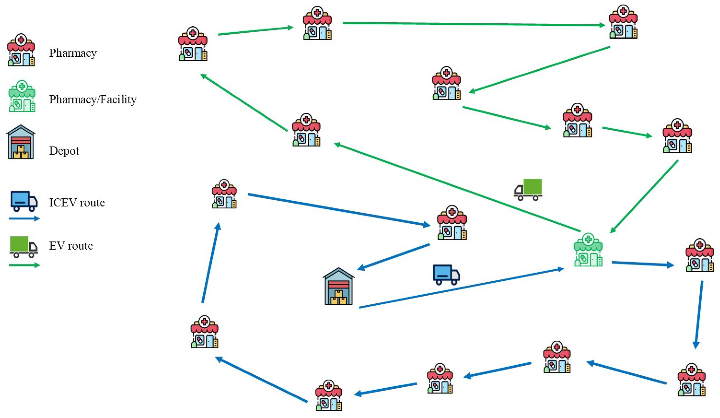
2.3. Problem Description

As outlined in Section 1.1, the medicine distribution problem under consideration can be formulated and solved independently for each geographical zone, which includes a subset of pharmacies (or customers) and a regional depot. To describe the mathematical formulation of the problem for each zone, the following assumptions are made:

• n: number of nodes, consisting of $(n-1)$ customers to be visited and the depot, referred to as $d_1$, from which the ICEV’s route originates and ends (hereafter also referred to as the first route);
• $d_2$: a customer that also serves as a depot for the EV’s route, selected from the customers served by the ICEV. The EV’s route is hereafter referred to as the second route;
• $a_{ij}$, $i,j=1,\dots ,n$: length of the best route to move from node i to node j using the ICEV;
• $b_{ij}$, $i,j=1,\dots ,n$: length of the best route to move from node i to node j using the EV. Since the EV may be authorized to cross low-emission zones in urban areas, it generally happens that $b_{ij}\le a_{ij}$, $i,j=1,\dots ,n$;
• $e_{ICEV}$ and $e_{EV}$: CO₂ emission (in kg/km) of the ICEV and EV, respectively;
• $c_{ICEV}$ and $c_{EV}$: transportation cost (in EUR/km) of the ICEV and EV, respectively. Although the trend in future years favors a reduction in the cost per kilometer for electric vehicles, it is more realistically assumed that $c_{ICEV}\le c_{EV}$, which implies that

  $$c_{EV}=(1+\alpha )c_{ICEV},$$

  (1)

  where $\alpha \ge 0$;
• k, $2\le k\le n$: number of customers and depot $d_1$ served by the first route.

A solution to this problem must determine

• the assignment of customers to the two vehicles, ensuring that each customer is served by only one vehicle. Specifically, the ICEV route starts and ends at depot $d_1$, while the EV route starts and ends at depot $d_2$;
• the visiting order of the customers within each route.

These decisions must be made with the objective of minimizing both CO₂ emissions and transportation costs. The delivery plan is subject to the following constraints:

• each vehicle can perform only one route that starts and ends at its designated depot;
• split deliveries are not allowed;
• the first node visited by the ICEV’s route must be node $d_2$ to ensure that the second tour can start as quickly as possible, thereby reducing the overall completion time for serving the customers.

As previously mentioned, n is assumed small enough to ensure it does not exceed vehicle capacity, the maximum allowable route duration due to driver working hours, or the EV’s battery range. Moreover, the twice-daily delivery schedule allows customers to avoid imposing specific time windows or due date constraints, as products are delivered within half a day of placing an order. These assumptions are reasonable in this context and enable the optimal use of the vehicle fleet in delivery planning.

Mathematical Model

The decision variables are the following. Associated with the first route: $x_{ij}$, $i,j=1,\dots ,n$, which are binary and equal to 1 if the path from i to j is part of the solution, and 0 otherwise; $z_j$, $j=1,\dots ,n$, also binary, which are equal to 1 if the corresponding node j is visited by the ICEV, and 0 otherwise; $u_j\ge 0$, $j=1,\dots ,n$, indicating the position of node j along the first route. By convention, $u_{d_1}=0$, and consequently, $u_j<k$, $j=1,\dots ,n$. Associated with the second route: $y_{ij}$, $i,j=1,\dots ,n$, which are binary and equal to 1 if the path from i to j is part of the solution, and 0 otherwise; $w_j$, $j=1,\dots ,n$, also binary, which are equal to 1 if the corresponding node j is visited by the EV, and 0 otherwise; $t_j\ge 0$, $j=1,\dots ,n$, indicating the position of node j along the second route. Since $t_{d_2}=0$, we have $t_j<(n-k+1)$, $j=1,\dots ,n$, where $(n-k+1)$ is the number of nodes that constitute the second route (note that $d_2$ belongs to both routes). In the case where $k=n$, this means that all customers are served by the ICEV, and thus the second route does not exist.

The bi-objective optimization model is formulated as follows.

$$\mathrm{Minimize}{e}_{ICEV}\sum _{i=1}^n\sum _{j=1}^n{a}_{ij}{x}_{ij}+e_{EV}\sum _{i=1}^n\sum _{j=1}^n{b}_{ij}{y}_{ij}$$

(2)

$$\mathrm{Minimize}{c}_{ICEV}\sum _{i=1}^n\sum _{j=1}^n{a}_{ij}{x}_{ij}+c_{EV}\sum _{i=1}^n\sum _{j=1}^n{b}_{ij}{y}_{ij}$$

(3)

subject to

$$\sum _{i=1}^n{x}_{ij}=z_j,j=1,\dots ,n$$

(4)

$$\sum _{j=1}^n{x}_{ij}=z_i,i=1,\dots ,n$$

(5)

$$u_i-u_j+k{x}_{ij}\le k-1,i,j=1,\dots ,n;i\ne j;j\ne d_1$$

(6)

$$u_j\le (k-1)z_j,j=1,\dots ,n$$

(7)

$$u_{d_2}=1$$

(8)

$$w_{d_2}=1$$

(9)

$$w_j=1-z_j,j=1,\dots ,n;j\ne d_2$$

(10)

$$\sum _{i=1}^n{y}_{ij}=w_j,j=1,\dots ,n$$

(11)

$$\sum _{j=1}^n{y}_{ij}=w_i,i=1,\dots ,n$$

(12)

$$t_i-t_j+(n-k+1)y_{ij}\le n-k,i,j=1,\dots ,n;i\ne j;j\ne d_2$$

(13)

$$t_j\le (n-k)w_j,j=1,\dots ,n$$

(14)

$$x_{ij},y_{ij}\in \{0,1\},i,j=1,\dots ,n$$

(15)

$$z_j,w_j\in \{0,1\},j=1,\dots ,n$$

(16)

$$u_j,t_j\ge 0,j=1,\dots ,n.$$

(17)

Objective functions (2) and (3) represent the total CO₂ emissions and transportation costs of both tours, respectively, both of which are to be minimized.

Constraints (4)–(6) ensure that the first tour is a Hamiltonian circuit on k nodes. Specifically, Equations (4) represent the incoming degree constraints, Equation (5) represents the outgoing degree constraints, while Constraints (6) prevent the generation of disconnected subcircuits.

Since there are multiple solutions for variables $u_j$ corresponding to the optimal solution, Constraints (7) ensure that $u_j$ is equal to 0 for all nodes j that are not part of the first tour, and that the value for the other vertices is consistent with the intended meaning of the variable.

Equation (8) ensures that the first node to be visited in the first tour is the depot node $d_2$ of the second tour. This guarantees that the second tour can start as quickly as possible, thereby reducing the completion time for serving the customers.

Equations (9) and (10) are used to determine the nodes that are served by the second tour. Constraints (11)–(14) are the corresponding constraints relative to (4)–(7) necessary for the construction of the second tour. Finally, Constraints (15)–(17) ensure that the decision variables are binary or continuous.

Note that in the formulation of model (2)–(17) it is necessary to ensure that it is not possible to visit a node immediately after leaving the same node. This can be achieved by considering the following additional constraints: $x_{jj}=0$ and $y_{jj}=0$, $j=1,\dots ,n$, or, equivalently, by setting $a_{jj}=b_{jj}=M$, $j=1,\dots ,n$, where M is a very large number relative to the actual distance values of the problem (we decided to follow the second alternative).

Model (2)–(17) is NP-hard, since its constraints can be viewed as an extension of those in the classic asymmetric traveling salesperson problem (ATSP). In the formulation under investigation, compared to the ATSP, there are two reduced Hamiltonian circuits, each determined on a subset of vertices and sharing a common node.

A variety of methods have been proposed in the literature to determine a set of Pareto optimal solutions for multi-objective optimization problems such as Model (2)–(17) (see Hwang and Masud [33]) The $ϵ$-constraint method has been applied. This is a posteriori method, in which a set of efficient solutions of the problem is generated and then the decision maker selects, from these, the preferred one. The method has been successfully applied in various practical applications [34,35]. A preliminary step is to transform Objective function (3) into a constraint as follows:

$$c_{ICEV}\sum _{i=1}^n\sum _{j=1}^n{a}_{ij}{x}_{ij}+c_{EV}\sum _{i=1}^n\sum _{j=1}^n{b}_{ij}{y}_{ij}\le B,$$

(18)

where B represents the available budget. The problem is then solved for different values of B chosen within the interval $[B_{min},B_{max}]$. A method to determine the values of $B_{min}$ and $B_{max}$ is illustrated later.

The resulting model is referred to in the sequel as two-echelon asymmetric salesperson problem (2-EATSP). The optimal solution of the 2-EATSP model for each value of B can be determined in acceptable times only for instances with number n of nodes that is not particularly high (on the order of thousands). However, many practical problems have a size well below these acceptable limits, allowing decision-makers to focus solely on the formulation of the model and the interpretation of the obtained results (i.e., managerial insights), rather than on the exact or approximate algorithms to be considered.

3. Results

This section is dedicated to computational experiments. Specifically, Section 3.1 provides a detailed description of the data used in the case study addressed in this paper. Section 3.2 presents the computational results obtained by applying the 2-EATSP model to the data provided by the LSP, along with a discussion of the various solutions proposed to meet the company’s requirements. Finally, Section 3.3 explores different scenarios in terms of vehicle transportation costs to demonstrate the effectiveness of the 2-EATSP model under more general operating conditions.

The 2-EATSP model was coded in Lingo, version 19.0 (https://www.lindo.com/). Lingo 19.0 is a powerful optimization software used for solving a variety of optimization problem types, including mixed-integer programming. Lingo uses a range of optimization method libraries. Specifically, for integer programming, Lingo employs the branch-and-bound method. For linear mixed-integer models, Lingo incorporates extensive pre-processing, adding cuts to reduce the non-integer feasible region, which helps to improve computational times for most mixed-integer programming models. For more details, see https://www.lindo.com/downloads/PDF/LINGO.pdf (accessed on 25 of August 2024).

The computer used for the computational experiments is equipped with an Intel Core i7-12700H processor, 32 GB of RAM, and Windows 11 Professional 64-bit.

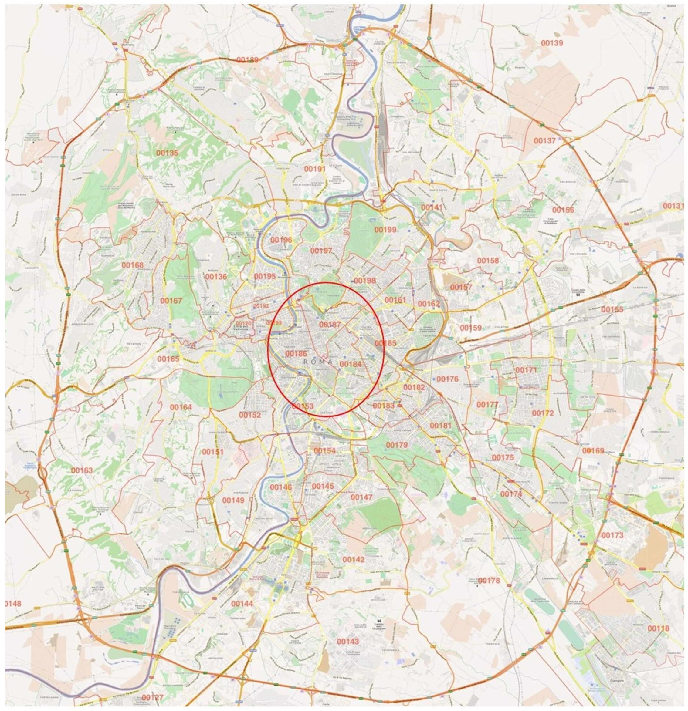
3.1. Data of the Case Study

Figure 2 highlights the city districts and the specific area selected for experimentation, where 30 pharmacies and a regional depot are located.

Table A1. Geographical coordinates of the 31 Points of Interest.

ID	Point of Interest	Latitude	Longitude
1	Pharmacy 1	41.8797075	12.5017273
2	Pharmacy 2	41.8815379	12.5131229
3	Pharmacy 3	41.8960212	12.4904504
4	Pharmacy 4	41.8889683	12.4964994
5	Pharmacy 5	41.8941843	12.4906858
6	Pharmacy 6	41.9025231	12.5016612
7	Pharmacy 7	41.9009856	12.4932650
8	Pharmacy 8	41.8984073	12.4905973
9	Pharmacy 9	41.8974436	12.4952554
10	Pharmacy 10	41.8951780	12.4997721
11	Pharmacy 11	41.8996024	12.4947634
12	Pharmacy 12	41.8950950	12.5009679
13	Pharmacy 13	41.8982191	12.5155031
14	Pharmacy 14	41.9022693	12.5049111
15	Pharmacy 15	41.8919719	12.5017881
16	Pharmacy 16	41.8941144	12.5033891
17	Pharmacy 17	41.8980393	12.4996115
18	Pharmacy 18	41.9015448	12.5031056
19	Pharmacy 19	41.8925406	12.5054307
20	Pharmacy 20	41.9053853	12.5038711
21	Pharmacy 21	41.8974293	12.5126908
22	Pharmacy 22	41.8950682	12.5053476
23	Pharmacy 23	41.8910022	12.5022499
24	Pharmacy 24	41.9012792	12.5022033
25	Pharmacy 25	41.8965883	12.5148512
26	Pharmacy 26	41.9029806	12.4957247
27	Pharmacy 27	41.8977001	12.5020334
28	Pharmacy 28	41.8937245	12.5077524
29	Pharmacy 29	41.8895619	12.5137454
30	Pharmacy 30	41.8906894	12.5063857
31	Regional depot	41.8864490	12.5159620

in Appendix A provides the geographical coordinates of the 31 Points of Interest.

The temperature-controlled ICEV has an estimated CO₂ emission of 0.3168 kg/km. The estimated CO₂ emission for the temperature-controlled EV is 0.05825 kg/km.

The intermediate facility, used as depot for the EV, is located near pharmacy ID 10. The distance between the intermediate facility and pharmacy ID 10 is negligible.

Each pharmacy is also associated with a service time. Since all pharmacies need to be served, the total service time is obviously constant; however, these times impact the service completion times of the two vehicles, as they depend on the number of pharmacies served by each of the two routes. The distributor sets the average service time as a constant for each pharmacy, equal to five minutes.

Similarly, service times for loading and unloading goods are assigned to each depot, with $d_1=31$ and $d_2=10$. Since the loads are not bulky, the time is also set to five minutes in this case.

In

Table A4. ICEV distance matrix (in km) of pharmacies and depot (ID 1 to ID 8).

From/To	ID 1	ID 2	ID 3	ID 4	ID 5	ID 6	ID 7	ID 8
ID 1	-	1.274	3.849	2.738	3.093	3.619	4.112	3.723
ID 2	1.681	-	3.604	2.780	3.113	3.567	3.795	3.478
ID 3	3.237	3.404	-	1.695	0.264	1.814	1.104	0.715
ID 4	2.183	2.485	3.909	-	3.153	3.680	4.173	3.783
ID 5	3.018	3.330	1.246	1.475	-	1.595	1.509	1.120
ID 6	3.960	3.653	2.579	3.947	2.517	-	1.919	2.453
ID 7	3.931	3.478	1.136	2.388	0.957	0.895	-	0.937
ID 8	3.643	3.810	0.848	2.100	0.669	1.285	0.389	-
ID 9	3.697	3.194	0.603	2.154	0.723	1.133	0.866	0.477
ID 10	2.915	2.566	1.521	2.196	0.765	1.365	1.784	1.395
ID 11	3.613	3.264	1.032	2.401	0.970	1.411	1.112	0.723
ID 12	2.939	2.590	1.619	2.294	0.863	1.389	1.882	1.493
ID 13	3.393	2.714	3.411	3.380	3.152	3.197	2.994	3.285
ID 14	3.890	3.583	2.674	3.877	2.448	1.879	1.538	2.383
ID 15	2.513	2.164	1.923	1.993	1.167	1.693	2.186	1.797
ID 16	2.517	2.210	1.638	2.504	1.097	1.600	1.828	1.511
ID 17	3.170	2.862	1.446	2.815	1.384	0.935	1.162	1.320
ID 18	3.792	3.485	2.412	3.779	2.350	2.093	1.752	2.285
ID 19	2.257	1.950	1.897	2.244	1.357	1.860	2.087	1.771
ID 20	4.332	4.025	2.296	3.547	2.116	1.501	1.159	2.096
ID 21	3.467	2.787	2.630	3.453	2.568	2.416	2.671	2.504
ID 22	3.218	2.911	1.710	3.079	1.648	1.496	1.724	1.584
ID 23	2.399	2.050	2.037	1.878	1.281	1.807	2.300	1.911
ID 24	3.952	3.644	2.733	3.939	2.509	1.939	1.597	2.445
ID 25	3.617	2.938	3.027	3.604	3.376	2.813	3.068	2.900
ID 26	4.262	3.769	1.467	2.719	1.288	0.673	0.331	1.267
ID 27	3.289	2.982	1.793	3.163	1.732	1.580	1.807	1.667
ID 28	2.584	2.379	2.515	2.570	1.975	2.314	2.541	2.389
ID 29	2.189	1.561	2.705	2.392	2.164	2.503	2.731	2.579
ID 30	2.037	1.730	2.117	2.024	1.577	2.080	2.308	1.991
ID 31	1.924	1.183	3.202	2.457	2.661	3.000	3.228	3.076

,

Table A5. ICEV distance matrix (in km) of pharmacies and depot (ID 9 to ID 16).

From/To	ID 9	ID 10	ID 11	ID 12	ID 13	ID 14	ID 15	ID 16
ID 1	3.108	2.328	3.087	2.352	3.286	3.841	1.926	2.586
ID 2	3.056	2.348	3.034	2.201	2.844	3.399	1.946	1.967
ID 3	1.740	0.985	1.091	1.082	3.006	2.335	1.386	1.317
ID 4	3.168	2.388	3.147	2.412	2.971	3.525	1.986	2.481
ID 5	1.520	0.765	1.496	0.863	2.786	2.115	1.167	1.097
ID 6	2.031	1.653	2.009	1.555	1.698	0.521	1.980	1.558
ID 7	0.546	0.943	0.214	1.038	3.197	1.416	1.314	1.298
ID 8	0.880	1.390	0.548	1.488	3.587	1.805	1.792	1.722
ID 9	-	0.659	0.853	0.754	2.704	1.654	1.030	1.014
ID 10	0.854	-	0.833	0.098	2.022	1.886	0.402	0.332
ID 11	1.344	1.932	-	0.824	2.773	1.932	1.100	1.084
ID 12	0.878	0.098	0.857	-	1.924	2.478	0.426	0.235
ID 13	2.862	2.388	2.841	2.290	-	1.529	2.547	2.055
ID 14	1.961	1.583	1.752	1.485	1.628	-	1.911	1.489
ID 15	1.182	0.402	1.161	0.426	2.000	2.555	-	0.660
ID 16	1.089	0.332	1.068	0.235	1.689	2.244	0.660	-
ID 17	0.897	0.747	0.876	0.649	2.342	1.455	1.075	0.653
ID 18	1.863	1.485	1.842	1.387	1.530	0.353	1.813	1.391
ID 19	1.349	0.592	1.327	0.494	1.587	2.142	0.920	0.260
ID 20	1.705	2.024	1.373	1.927	1.520	0.638	2.352	1.930
ID 21	2.081	1.703	2.060	1.605	0.306	1.205	2.031	1.609
ID 22	1.161	0.795	1.140	0.697	1.659	2.214	1.123	0.701
ID 23	1.296	0.516	1.275	0.540	1.886	2.441	0.114	0.774
ID 24	2.022	1.644	1.811	1.547	1.690	0.513	1.972	1.550
ID 25	2.478	2.612	2.457	2.514	0.388	1.602	2.771	2.279
ID 26	0.877	1.234	0.545	1.329	2.370	1.193	1.605	1.450
ID 27	1.245	0.867	1.223	0.769	1.973	2.528	1.195	0.772
ID 28	1.967	1.210	1.945	1.112	1.215	1.770	1.538	0.878
ID 29	2.156	1.400	2.135	1.302	1.633	2.187	1.728	1.067
ID 30	1.569	0.812	1.547	0.714	1.650	2.204	1.140	0.480
ID 31	2.653	1.897	2.632	1.799	2.146	2.701	1.624	1.564

,

Table A6. ICEV distance matrix (in km) of pharmacies and depot (ID 17 to ID 24).

From/To	ID 17	ID 18	ID 19	ID 20	ID 21	ID 22	ID 23	ID 24
ID 1	3.067	3.777	2.425	4.139	2.981	2.772	1.812	3.723
ID 2	3.015	3.866	1.707	4.149	2.538	2.055	1.832	3.812
ID 3	1.262	1.972	1.577	2.334	2.701	1.767	1.501	1.918
ID 4	3.127	3.837	2.221	4.275	2.665	2.569	1.872	3.783
ID 5	1.042	1.752	1.357	2.114	2.481	1.547	1.281	1.698
ID 6	1.989	0.158	1.818	1.204	1.262	1.463	2.095	0.103
ID 7	0.898	1.053	1.558	1.422	2.157	1.748	1.428	0.999
ID 8	1.232	1.442	1.982	1.811	2.547	2.172	1.906	1.388
ID 9	0.581	1.291	1.274	1.653	2.398	1.464	1.144	1.237
ID 10	0.813	1.523	0.592	1.885	1.716	0.782	0.516	1.469
ID 11	0.684	1.569	1.344	1.931	2.468	1.534	1.214	1.515
ID 12	0.837	1.547	0.494	1.909	1.618	0.684	0.540	1.493
ID 13	2.821	1.996	2.005	2.279	0.306	1.701	2.433	1.942
ID 14	1.920	0.465	1.748	0.822	1.193	1.394	2.025	0.411
ID 15	1.141	1.851	0.848	2.213	1.695	1.110	0.114	1.797
ID 16	1.048	1.758	0.260	2.120	1.384	0.450	0.774	1.704
ID 17	-	1.092	0.912	1.454	2.036	1.103	1.189	1.038
ID 18	1.822	-	1.650	1.036	1.094	1.296	1.927	0.766
ID 19	1.307	2.018	-	2.380	1.281	0.348	1.034	1.964
ID 20	1.623	0.581	2.190	-	1.351	1.835	2.466	0.527
ID 21	2.040	1.673	1.869	1.955	-	1.514	2.145	1.618
ID 22	1.120	1.654	0.961	2.016	1.354	-	1.237	1.600
ID 23	1.255	1.965	0.734	2.327	1.581	1.082	-	1.911
ID 24	1.981	0.149	1.810	0.881	1.254	1.455	2.086	-
ID 25	2.437	2.069	2.230	2.352	0.397	1.925	2.657	2.015
ID 26	0.795	0.830	1.710	1.199	1.935	1.569	1.719	0.776
ID 27	1.203	1.737	1.032	2.099	1.668	0.911	1.309	1.683
ID 28	1.925	2.237	0.822	2.520	0.909	0.817	1.652	2.183
ID 29	2.115	2.655	1.012	2.937	1.327	1.007	1.445	2.600
ID 30	1.527	2.238	0.220	2.954	1.344	0.568	1.254	2.184
ID 31	2.612	3.168	1.509	3.451	1.840	1.504	1.509	3.114

and

Table A7. ICEV distance matrix (in km) of pharmacies and depot (ID 25 to ID 31).

From/To	ID 25	ID 26	ID 27	ID 28	ID 29	ID 30	ID 31
ID 1	3.250	5.143	3.249	2.787	2.392	2.205	2.401
ID 2	2.441	4.214	2.532	2.069	1.195	1.487	0.807
ID 3	2.970	2.234	1.856	1.781	2.384	1.797	3.098
ID 4	2.935	4.987	3.045	2.583	2.420	2.001	2.883
ID 5	2.750	2.748	1.636	1.562	2.164	1.577	3.024
ID 6	1.532	2.112	1.177	1.496	2.241	1.978	3.354
ID 7	2.427	1.132	1.272	1.763	2.365	1.778	3.172
ID 8	2.816	1.628	1.662	2.187	2.789	2.202	3.503
ID 9	2.667	2.105	1.175	1.479	2.082	1.494	2.888
ID 10	1.986	3.023	1.259	0.797	1.400	0.812	2.259
ID 11	2.737	2.351	1.106	1.549	2.151	1.564	2.957
ID 12	1.888	2.036	1.161	0.699	1.302	0.714	2.786
ID 13	0.508	3.309	1.552	2.010	1.362	1.785	2.313
ID 14	1.462	1.731	1.108	1.427	2.172	1.909	3.285
ID 15	1.964	2.340	1.587	1.125	1.251	0.628	1.858
ID 16	1.653	2.247	0.927	0.465	1.067	0.480	2.551
ID 17	2.306	1.581	0.604	1.117	1.720	1.132	3.204
ID 18	1.364	1.945	1.010	1.329	2.074	1.811	3.187
ID 19	1.551	2.507	0.824	0.362	0.965	0.220	2.449
ID 20	1.620	1.352	1.549	1.868	2.613	2.350	3.726
ID 21	0.347	2.985	1.228	1.547	1.436	1.859	2.386
ID 22	1.623	2.143	0.477	0.602	1.347	1.181	2.580
ID 23	1.850	2.454	1.558	1.096	1.137	0.514	1.743
ID 24	1.523	1.790	1.169	1.488	2.233	1.970	3.346
ID 25	-	3.382	1.625	2.234	1.587	2.010	2.537
ID 26	2.204	-	1.049	1.602	2.517	1.930	3.580
ID 27	1.937	2.226	-	0.944	1.689	1.252	2.922
ID 28	1.179	2.960	1.294	-	1.027	0.602	1.978
ID 29	1.399	3.150	1.484	1.022	100 -	0.792	1.484
ID 30	1.614	2.727	1.044	0.582	0.682	-	1.423
ID 31	1.743	3.647	1.981	1.519	0.497	1.289	-

, the values of $a_{ij}$, $i,j=1,\dots ,31$ are reported. Similarly,

Table A8. EV distance matrix (in km) of pharmacies and depot (ID 1 to ID 8).

From/To	ID 1	ID 2	ID 3	ID 4	ID 5	ID 6	ID 7	ID 8
ID 1	-	1.274	2.848	1.774	2.112	2.548	3.187	2.885
ID 2	1.681	-	2.586	1.960	2.467	2.507	2.932	2.746
ID 3	2.494	2.195	-	1.695	0.264	1.814	1.104	0.715
ID 4	1.632	1.833	2.957	-	2.104	2.734	3.150	2.698
ID 5	2.106	2.191	1.246	1.475	-	1.595	1.509	1.120
ID 6	2.897	2.907	2.018	3.138	1.758	-	1.919	1.839
ID 7	3.097	2.621	1.136	1.848	0.957	0.895	-	0.937
ID 8	2.805	2.504	0.848	1.499	0.669	1.285	0.389	-
ID 9	2.954	2.294	0.603	1.579	0.723	1.133	0.866	0.477
ID 10	2.004	1.904	1.521	1.416	0.765	1.365	1.784	1.395
ID 11	2.716	2.462	1.032	1.907	0.970	1.411	1.112	0.723
ID 12	2.283	1.869	1.619	1.473	0.863	1.389	1.882	1.493
ID 13	2.585	1.855	2.528	2.362	2.202	2.284	2.352	2.189
ID 14	3.026	2.671	2.090	2.528	1.614	1.879	1.538	1.808
ID 15	1.797	1.647	1.923	1.993	1.167	1.693	1.716	1.797
ID 16	1.877	1.645	1.638	1.712	1.097	1.600	1.828	1.511
ID 17	2.493	2.216	1.446	1.847	1.384	0.935	1.162	1.320
ID 18	3.031	2.698	1.718	2.605	1.635	1.599	1.752	1.568
ID 19	1.536	1.950	1.897	1.562	1.357	1.860	1.386	1.771
ID 20	3.297	2.593	1.693	2.332	1.479	1.501	1.159	1.410
ID 21	2.416	2.151	1.708	2.235	1.678	1.790	2.130	1.631
ID 22	2.411	2.250	1.710	2.189	1.648	1.496	1.724	1.584
ID 23	1.683	1.315	1.584	1.878	1.281	1.807	1.649	1.911
ID 24	2.718	2.705	2.058	2.641	1.682	1.939	1.597	1.617
ID 25	2.518	2.020	2.037	2.370	2.518	2.081	2.408	2.052
ID 26	3.048	2.689	1.467	1.898	1.288	0.673	0.331	1.267
ID 27	2.213	2.257	1.793	2.308	1.732	1.580	1.807	1.667
ID 28	1.779	1.747	1.942	1.992	1.975	1.758	1.810	1.638
ID 29	1.557	1.561	1.899	1.753	1.645	1.859	1.854	2.057
ID 30	1.476	1.730	1.635	1.479	1.577	1.531	1.619	1.991
ID 31	1.924	1.183	2.123	1.707	2.060	2.366	2.250	2.448

,

Table A9. EV distance matrix (in km) of pharmacies and depot (ID 9 to ID 16).

From/To	ID 9	ID 10	ID 11	ID 12	ID 13	ID 14	ID 15	ID 16
ID 1	2.457	1.539	2.173	1.615	2.618	2.477	1.926	1.725
ID 2	1.981	1.515	2.035	1.654	2.231	2.347	1.946	1.967
ID 3	1.740	0.985	1.091	1.082	2.032	1.517	1.386	1.317
ID 4	2.463	1.604	2.480	1.549	2.010	2.708	1.986	1.983
ID 5	1.520	0.765	1.496	0.863	2.018	1.652	1.167	1.097
ID 6	1.460	1.653	1.315	1.555	1.698	0.521	1.980	1.558
ID 7	0.546	0.943	0.214	1.038	2.082	1.416	1.314	1.298
ID 8	0.880	1.390	0.548	1.488	2.407	1.805	1.792	1.722
ID 9	-	0.659	0.853	0.754	2.067	1.654	1.030	1.014
ID 10	0.854	-	0.833	0.098	1.307	1.886	0.402	0.332
ID 11	0.332	0.729	-	0.824	1.948	1.932	1.100	1.084
ID 12	0.878	0.098	0.857	-	1.924	1.886	0.426	0.235
ID 13	2.143	1.839	2.254	1.615	-	1.529	1.762	1.639
ID 14	1.961	1.583	1.752	1.485	1.628	-	1.911	1.489
ID 15	1.182	0.402	1.161	0.426	2.000	1.677	-	0.660
ID 16	1.089	0.332	1.068	0.235	1.689	1.473	0.660	-
ID 17	0.897	0.747	0.876	0.649	1.647	1.455	1.075	0.653
ID 18	1.863	1.485	1.842	1.387	1.530	0.353	1.813	1.391
ID 19	1.349	0.592	1.327	0.494	1.587	1.489	0.920	0.260
ID 20	1.705	1.456	1.373	1.927	1.520	0.638	1.665	1.930
ID 21	1.522	1.703	1.329	1.605	0.306	1.205	1.312	1.609
ID 22	1.161	0.795	1.140	0.697	1.659	1.439	1.123	0.701
ID 23	1.296	0.516	1.275	0.540	1.886	1.610	0.114	0.774
ID 24	1.322	1.644	1.811	1.547	1.690	0.513	1.972	1.550
ID 25	1.968	1.895	1.753	1.896	0.388	1.602	1.955	1.812
ID 26	0.877	1.234	0.545	1.329	1.621	1.193	1.605	1.450
ID 27	1.245	0.867	1.223	0.769	1.973	1.990	1.195	0.772
ID 28	1.967	1.210	1.945	1.112	1.215	1.770	1.538	0.878
ID 29	1.685	1.400	1.692	1.302	1.633	1.736	1.728	1.067
ID 30	1.569	0.812	1.547	0.714	1.650	1.539	1.140	0.480
ID 31	1.873	1.897	1.710	1.799	1.519	1.993	1.624	1.564

,

Table A10. EV distance matrix (in km) of pharmacies and depot (ID 17 to ID 24).

From/To	ID 17	ID 18	ID 19	ID 20	ID 21	ID 22	ID 23	ID 24
ID 1	2.350	2.912	1.869	3.110	2.135	2.026	1.812	2.805
ID 2	2.200	3.018	1.707	2.990	2.016	1.345	1.832	2.892
ID 3	1.262	1.972	1.577	1.533	1.903	1.767	1.501	1.918
ID 4	2.094	2.636	1.518	2.892	2.100	1.908	1.872	2.956
ID 5	1.042	1.752	1.357	1.450	1.683	1.547	1.281	1.698
ID 6	1.989	0.158	1.818	1.204	1.262	1.463	1.592	0.103
ID 7	0.898	1.053	1.558	1.422	1.447	1.748	1.428	0.999
ID 8	1.232	1.442	1.982	1.811	1.673	1.627	1.906	1.388
ID 9	0.581	1.291	1.274	1.653	1.872	1.464	1.144	1.237
ID 10	0.813	1.523	0.592	1.885	1.716	0.782	0.516	1.469
ID 11	0.684	1.569	1.344	1.931	1.776	1.534	1.214	1.515
ID 12	0.837	1.547	0.494	1.909	1.618	0.684	0.540	1.493
ID 13	2.026	1.996	1.531	1.588	0.324	1.701	1.878	1.942
ID 14	1.920	0.465	1.748	0.822	1.193	1.394	1.406	0.411
ID 15	1.141	1.851	0.848	1.451	1.695	1.110	0.114	1.797
ID 16	1.048	1.758	0.260	1.395	1.384	0.450	0.774	1.704
ID 17	-	1.092	0.912	1.454	1.626	1.103	1.189	1.038
ID 18	1.822	-	1.650	1.036	1.094	1.296	1.927	0.766
ID 19	1.307	1.431	-	1.868	1.281	0.348	1.034	1.964
ID 20	1.623	0.581	1.579	-	1.351	1.835	1.896	0.527
ID 21	1.354	1.673	1.869	1.955	-	1.514	1.615	1.618
ID 22	1.120	1.654	0.961	1.388	1.354	-	1.237	1.600
ID 23	1.255	1.965	0.734	1.586	1.581	1.082	-	1.911
ID 24	1.981	0.149	1.810	0.881	1.254	1.455	1.498	-
ID 25	1.935	1.383	1.655	1.834	0.397	1.925	1.904	1.364
ID 26	0.795	0.830	1.710	1.199	1.935	1.569	1.719	0.776
ID 27	1.203	1.737	1.032	1.670	1.668	0.911	1.309	1.683
ID 28	1.925	1.554	0.822	1.903	0.909	0.817	1.652	1.413
ID 29	1.403	1.825	1.012	2.127	1.327	1.007	1.445	2.039
ID 30	1.527	1.774	0.220	2.186	1.344	0.568	1.254	1.528
ID 31	1.821	2.302	1.509	2.460	1.840	1.504	1.509	2.022

and

Table A11. EV distance matrix (in km) of pharmacies and depot (ID 25 to ID 31).

From/To	ID 25	ID 26	ID 27	ID 28	ID 29	ID 30	ID 31
ID 1	2.282	3.999	2.447	2.067	1.739	1.487	1.844
ID 2	1.694	3.161	1.815	1.474	1.195	1.487	0.807
ID 3	1.938	1.755	1.856	1.781	1.832	1.797	2.456
ID 4	1.943	3.493	2.275	2.04	1.816	1.497	1.97
ID 5	1.953	1.859	1.636	1.562	1.56	1.577	2.166
ID 6	1.532	1.551	1.177	1.496	1.522	1.978	2.56
ID 7	1.696	1.132	1.272	1.763	1.562	1.778	2.13
ID 8	2.203	1.628	1.662	1.67	2.04	1.474	2.32
ID 9	1.99	1.366	1.175	1.479	1.558	1.494	2.07
ID 10	1.986	2.296	1.259	0.797	1.4	0.812	1.627
ID 11	2.167	1.776	1.106	1.549	1.408	1.564	2.253
ID 12	1.888	1.41	1.161	0.699	1.302	0.714	1.889
ID 13	0.508	2.281	1.552	1.484	1.362	1.785	1.503
ID 14	1.462	1.731	1.108	1.427	1.454	1.909	2.336
ID 15	1.964	1.635	1.587	1.125	1.251	0.628	1.858
ID 16	1.653	1.518	0.927	0.465	1.067	0.48	1.779
ID 17	1.808	1.581	0.604	1.117	1.72	1.132	2.223
ID 18	1.364	1.945	1.01	1.329	1.58	1.811	2.384
ID 19	1.551	1.858	0.824	0.362	0.965	0.22	1.855
ID 20	1.62	1.352	1.549	1.868	1.788	1.774	2.967
ID 21	0.347	2.204	1.228	1.547	1.436	1.859	1.584
ID 22	1.623	1.519	0.477	0.602	1.347	1.181	2.024
ID 23	1.85	1.689	1.558	1.096	1.137	0.514	1.743
ID 24	1.523	1.79	1.169	1.488	1.607	1.97	2.25
ID 25	-	2.589	1.625	1.564	1.587	1.581	2.009
ID 26	1.419	-	1.049	1.602	1.806	1.93	2.679
ID 27	1.937	1.438	-	0.944	1.689	1.252	1.947
ID 28	1.179	2.019	1.294	-	1.027	0.602	1.978
ID 29	1.399	2.272	1.484	1.022	-	0.792	1.484
ID 30	1.614	1.962	1.044	0.582	0.682	-	1.423
ID 31	1.743	2.693	1.981	1.519	0.497	1.289	-

indicate the values of $b_{ij}$, $i,j=1,\dots ,31$. For geospatial information, specifically vertex positions and travel distances, a Python routine integrated with Google Maps is used. Travel times are recorded every two hours during a working day, from 8:00 a.m. to 8:00 p.m., and the average value is used for the analysis.

The average speed $\overline{v}$ of a van (both ICEV and EV) in the city of Rome is estimated at 9 km/h. This low speed can be attributed to several factors characteristic of urban environments. Firstly, Rome is known for its historical and narrow streets, which limit the maneuverability and speed of larger vehicles like vans. Secondly, the city experiences high traffic congestion, especially during peak hours, further reducing average speeds. Additionally, frequent stops at traffic lights and pedestrian crossings, combined with the need to navigate around parked cars and other obstacles, contribute to slower travel times.

Regarding the transportation costs for the two vehicles, two scenarios are considered:

• $\alpha =0$ in Equation (1). In this scenario, there are no differences in the transportation cost per kilometer between the ICEV and the EV. This is evident from the data provided by the LSP and presented in

  Table A2. Cost comparison of ICEV and EV.

  Cost Component	ICEV [EUR/km]	EV [EUR/km]
  Fuel/Electricity	0.16	0.12
  Maintenance	0.05	0.06
  Other Operational Costs	0.03	0.04
  Amortized Purchase Cost	0.10	0.12
  Total Cost	0.34	0.34

  in Appendix A (the cost breakdown includes fuel consumption, maintenance, other operational expenses, and the purchase cost amortized over eight years). The 2-EATSP model can therefore be simplified by removing the budget constraint (18) and focusing solely on minimizing CO₂ emissions (see Section 3.2);
• $\alpha >0$ in Equation (1). In this more general scenario, several Pareto-optimal solutions can be generated for different values of budget B in Constraint (18). These solutions are evaluated and compared in a what-if analysis presented in Section 3.3.

3.2. Case of $\alpha =0$

Thirty runs of the Lingo model were performed, one for each choice of parameter $k\in [2,31]$. In all cases, the optimal solution to the problem was obtained, with a relatively short computational time, ranging from 0.59 s (when $k=31$) to 800.44 s (when $k=17$). The results obtained are shown in

Table 2. Computational results for values of k from 2 to 31.

	First Tour			Second Tour			Total
	$\overbrace{}$			$\overbrace{}$			$\overbrace{}$
k	Length	SCT	Emission	Length	SCT	Emission	Length	SCT	Emission	Time
	[km]	[h]	[kg/km]	[km]	[h]	[kg/km]	[km]	[h]	[kg/km]	[s]
2	4.156	0.712	1.317	19.202	4.928	1.119	23.358	4.928	2.435	1.11
3	4.132	0.792	1.309	19.202	4.844	1.119	23.334	4.844	2.428	4.75
4	4.156	0.878	1.317	18.502	4.683	1.078	22.658	4.683	2.394	4.00
5	4.132	0.959	1.309	18.952	4.650	1.104	23.084	4.650	2.413	3.00
6	4.133	1.043	1.309	18.830	4.553	1.097	22.963	4.553	2.406	2.57
7	4.876	1.208	1.545	17.973	4.374	1.047	22.849	4.374	2.592	10.55
8	5.091	1.316	1.613	18.135	4.309	1.056	23.226	4.309	2.669	9.10
9	5.834	1.482	1.848	17.278	4.131	1.006	23.112	4.131	2.855	11.67
10	6.423	1.630	2.035	16.775	3.991	0.977	23.198	3.991	3.012	36.31
11	7.092	1.788	2.247	15.875	3.808	0.925	22.967	3.808	3.171	27.24
12	7.842	1.955	2.484	15.027	3.630	0.875	22.869	3.630	3.360	42.00
13	8.484	2.109	2.688	14.063	3.440	0.819	22.547	3.440	3.507	477.26
14	9.071	2.258	2.874	14.056	3.356	0.819	23.127	3.356	3.692	234.38
15	9.821	2.425	3.111	12.889	3.143	0.751	22.710	3.143	3.862	218.47
16	10.002	2.528	3.169	14.541	3.243	0.847	24.543	3.243	4.016	450.54
17	10.291	2.643	3.260	14.980	3.209	0.873	25.271	3.209	4.133	800.44
18	10.918	2.796	3.459	14.206	3.039	0.827	25.124	3.039	4.286	347.18
19	11.632	2.959	3.685	12.962	2.818	0.755	24.594	2.959	4.440	204.61
20	12.127	3.097	3.842	12.270	2.657	0.715	24.397	3.097	4.557	120.87
21	12.634	3.237	4.002	12.003	2.544	0.699	24.637	3.237	4.702	108.72
22	13.194	3.383	4.180	11.319	2.385	0.659	24.513	3.383	4.839	50.18
23	13.916	3.546	4.409	9.977	2.153	0.581	23.893	3.546	4.990	35.57
24	14.659	3.712	4.644	9.224	1.986	0.537	23.883	3.712	5.181	31.78
25	15.428	3.881	4.888	8.431	1.814	0.491	23.859	3.881	5.379	27.77
26	16.242	4.055	5.145	7.011	1.573	0.408	23.253	4.055	5.554	26.87
27	16.685	4.187	5.286	7.315	1.524	0.426	24.000	4.187	5.712	26.10
28	17.407	4.351	5.515	5.837	1.276	0.340	23.244	4.351	5.855	7.58
29	18.291	4.532	5.795	4.587	1.054	0.267	22.878	4.532	6.062	3.86
30	20.193	4.827	6.397	3.020	0.796	0.176	23.213	4.827	6.573	1.29
31	21.606	5.067	6.845	0.000	0.000	0.000	21.606	5.067	6.845	0.59

.

3.2.1. Discussion

Regarding the service completion time ($SCT$), it is given by the maximum of the service completion times for the two tours, i.e.,

$$SCT=max\{SC{T}_1,SC{T}_2\}.$$

The $SC{T}_2$ takes into account the time to perform the second tour and the time shift for starting. This includes the service time of five minutes required for loading the ICEV at depot $d_1$ (equal to $0.08\overline{3}$ h), the time taken by the ICEV to reach $d_2=10$ (equal to ${\displaystyle \frac{a_{31,10}}{\overline{v}}}={\displaystyle \frac{1.897}{9}}=0.210\overline{7}$ h), and the service time for unloading the ICEV and loading the EV, again equal to $0.08\overline{3}$ h.

Since the distributor is interested in both reducing CO₂ emissions and minimizing $SCT$, the analysis of the results is focused on the values reported in the last two columns of Table 2 as parameter k varies. These results are better illustrated in Figure 3.

There is a clear inverse relationship between CO₂ emissions and $SCT$. As CO₂ emissions increase, $SCT$ generally decreases, which suggests that quicker service completion tends to result in higher CO₂ emissions.

For k values from 23 to 31, it is possible to see CO₂ emissions greater than 4.839 kg/km. This group has relatively high $SCT$ ranging from 3.3 to 5.1 h, indicating that these are less efficient solutions in terms of CO₂ emissions. Within this group, $SCT$ generally increases with increasing CO₂ emissions.

For k values from two to six, the CO₂ emissions are below 2.5 kg/km, but $SCT$ is higher (between 4.5 and 5 h). This group represents solutions with low CO₂ emissions but longer $SCT$. The range of $SCT$ in this group narrows as we approach lower CO₂ emissions.

From $k=7$ to $k=22$, we observe a middle ground where there is a gradual trade-off between CO₂ emissions and $SCT$. Here, CO₂ emissions range from 2.592 to 4.839 kg/km, and $SCT$ ranges from 2.9591 to 4.3744 h. In this group, as k increases, CO₂ emissions increase while $SCT$ decreases.

There is a noticeable elbow point around $k=15$ to $k=17$, where there is a significant reduction in $SCT$ without a dramatic increase in CO₂ emissions. This region might be considered an optimal trade-off between the two objectives.

The non-dominated solutions (i.e., solutions for which no other solution is better in both $SCT$ and CO₂ emissions) are obtained for the following values of k: 4, 6, 7, 8, 9, 10, 11, 12, 13, 14, 15, 18, and 19.

Considering the data and their insights, we can identify three solutions that seem to offer the best trade-offs. If the priority is to reduce CO₂ emissions, then $k=9$ might be the best choice. If the main priority is minimizing $SCT$, then $k=19$ could be the optimal choice, accepting higher CO₂ emissions. If a more balanced approach between both metrics is desired, $k=15$ offers a reasonable compromise between reduced $SCT$ and moderate CO₂ emissions. The choice of $k=15$ is adopted by the distributor. Figure 4 depicts the two tours obtained. In the figure, the tour associated with the ICEV is shown in black, while the tour associated with the EV is depicted in green. It can be observed that the two routes have a well-defined spatial arrangement, dividing the distribution zone into two main portions: on the right, the majority of the vertices are covered by the ICEV (area around the regional depot), while on the left, the majority of the vertices are covered by the EV. There is a partial overlap of the two routes only at vertices 19 and 23. Node 10 acts as a centroid for the two routes. Finally, note that the choice to serve Node 10 as the first customer on the ICEV route helps to reduce the total delivery time, especially when k and $(n-k)$ are balanced quantities, since the second vehicle does not have to wait long to receive the freight and the routes are executed almost simultaneously.

3.2.2. Benchmark Comparison

As aforementioned, considering the data and their insights, we can identify three solutions that seem to offer the best trade-offs: $k=9$, $k=19$, and $k=15$. To further illustrate the effectiveness of these solutions, we benchmark them against the extreme cases of $k=2$ and $k=31$. The solution with $k=2$ represents the scenario with the minimal number of customers served by the ICEV, resulting in the lowest CO₂ emissions. Conversely, $k=31$ represents the scenario where all customers are served by the ICEV, achieving the highest CO₂ emissions (in this case, the 2-EATSP is equivalent to the ATSP).

Table A3. Benchmark and best trade-off results on CO₂ emissions and $SCT$.

k	CO2 [kg/km]	STC [h]
2	2.435	4.928
9	2.855	4.131
15	3.862	3.143
19	4.440	2.959
31	6.845	5.067

provides an overview of the results for benchmark and best trade-off solutions, also graphically represented in Figure 5.

The figure shows the trend of total CO₂ emissions and $SCT$, given certain values of k. In particular, it can be observed that the green curve, representing the CO₂ emissions, has an increasing trend as k increases, since serving a greater number of nodes with ICEV leads to higher emissions. Conversely, the $SCT$ value is high in extreme cases, while it decreases towards a minimum point (at $k=19$) in trade-off cases. This trend is justified by the fact that solutions seeking a balance in the use of the two vehicles allow for simultaneous operation on the two routes, thus reducing the total service time.

From the CO₂ emissions perspective, the solution with $k=2$ has the lowest CO₂ emissions. Increasing k to nine results in a 17.2% increase in CO₂ emissions compared to $k=2$ while still maintaining relatively low emissions. At $k=15$, there is a more significant jump in CO₂ emissions, 35.3% higher than at $k=9$. Finally, at $k=19$, emissions increase by another 15%, and by the time $k=31$ is reached, emissions are 180.8% higher than in the case of $k=2$.

From the $SCT$ perspective, the solutions with $k=2$ and $k=31$ result in the highest $SCT$ values, at 4.928 h and 5.067 h, respectively. For $k=9$, $SCT$ decreases by 16.2% compared to $k=2$, showing significant improvement. Further improvement is seen with $k=15$, reducing $SCT$ by 21.6% from $k=2$; with $k=19$, the lowest $SCT$ is achieved, 42.8% lower than $k=2$ and 27.1% lower than $k=15$.

The analysis conducted further reinforces the previous findings: the identified trade-off solutions significantly improve the benchmark values of the extreme cases. Notably, prior to the purchase of the EV, the company’s activity can be identified in the case of $k=31$. The analysis highlights the importance of using the vehicles in synergy, even compared to the complete dismission of ICEV. As already mentioned, the best trade-off is represented by the solution obtained with $k=15$, which strikes a balance with moderate emissions and $SCT$, making it an optimal choice for achieving sustainability and efficiency. However, management attitudes more inclined to prioritize service level or sustainability might still encourage the use of one of the other two solutions, which are equally effective in terms of the considered indicators.

3.3. Case of $\alpha >0$

The value of $\alpha$ is chosen within the range $(0;1]$, which assumes that the transportation cost per kilometer for an EV can be up to twice the cost per kilometer for an ICEV. For each selected value of $\alpha$, the bounds $B_{min}$ and $B_{max}$ can be easily determined by solving the 2-EATSP removing Constraint (18) and setting k to 31 and 2, respectively. The budget value corresponding to the optimal solution obtained by setting $k=2$ (where only the customer located at node $d_2$ is served by the ICEV) is set as $B_{max}$, while the budget value obtained when $k=31$ (where all customers are served only by the ICEV) is used to determine $B_{min}$.

The value of B can then be chosen using the following formula:

$$B=B_{min}+\beta (B_{max}-B_{min}),$$

where parameter $\beta$ is selected within the range $[0;1]$.

A considerable number of Pareto-optimal solutions can therefore be generated for each $k\in [2,31]$ by setting $\alpha$, for example, to 0.25, 0.50, 0.75, and 1.00, and $\beta$ to 0.0, 0.25, 0.75, and 1.00, respectively. In the following discussion, for brevity, only a subset of the most interesting results is reported, specifically for k equal to 9, 15, and 19, with $\alpha$ set to 0.25 and 0.50, and $\beta =0.75$. These results can be compared with the most significant ones obtained when $\alpha =0$ and discussed in more detail in the previous section.

The results are summarized in

Table 3. Computational results for specific values of k, $\alpha$ and $\beta$.

k	α	β	B	SCT	GAPSCT	CO2	GAPCO2	cost	GAPcost
			[EUR]	[h]	[%]	[kg/km]	[%]	[EUR]	[%]
9	0.25	0.75	8.95	3.917	−5.18	3.171	11.07	8.90	15.32
9	0.50	0.75	10.16	3.791	−8.21	3.385	18.56	9.92	28.57
15	0.25	0.75	8.95	3.143	0.00	3.862	0.00	8.75	15.39
15	0.50	0.75	10.16	3.143	0.00	3.862	0.00	9.84	29.72
19	0.25	0.75	8.95	3.026	2.25	4.533	2.10	8.90	8.32
19	0.50	0.75	10.16	2.988	0.97	4.453	0.29	9.97	21.44

. The columns GAP_SCT, GAP_CO2, and GAP_cost report the percentage gap with respect to the corresponding optimal solution when $\alpha =0$.

The structure of the table facilitates a comparison across different cases, making it easier to identify Pareto-optimal solutions that balance the trade-offs between $SCT$, CO₂ emissions, and $cost$.

In the case of $k=9$, where 22 out of 30 customers are served by the EV, the increased transportation cost associated with using the EV leads to a reduction in $SCT$, along with a corresponding increase in CO₂ emissions and overall transportation costs. The more distant customers are served by the ICEV, the less expensive vehicle. This strategy helps to decrease the $SCT$ by reducing the difference in route lengths between the two vehicles.

For example, when $\alpha =0.50$, the solution results in a relatively high cost increase (+28.57%) and CO₂ emissions (+18.56%), but also demonstrates a significant reduction in $SCT$ (−8.21%). This can be clearly explained by considering the lengths of the two tours: 8.068 km for the first one (served by the ICEV) compared to 5.834 km (+38.29%) and 14.226 km for the second tour performed by the EV, versus 17.278 km (−21.45%), for a total of 22.294 km, compared to 23.112 km (−3.67%) in the solution where the transportation costs per kilometer are identical for both vehicles.

The solution obtained with $k=15$, where the number of customers served by each vehicle is more balanced, is cost-invariant. As the cost of the EV increases, both $SCT$ and CO₂ emissions remain unchanged because the optimal solution does not vary.

Finally, when $k=19$, a larger number of customers is served by the ICEV. Consequently, as the transportation cost per kilometer for the EV increases, the solution assigns the less distant customers to the ICEV, leading to a slight increase in both CO₂ emissions and service completion times. These increases remain modest, around 3%, due to the budget constraint.

The Pareto analysis conducted offers a comprehensive view of how varying parameters affect the trade-offs between multiple objectives. By examining different values of $\alpha$ and $\beta$, as well as varying budgets, the analysis provides a detailed understanding of how each parameter influences the three key performance indicators: $SCT$, CO₂ emissions, and transportation costs. This capability is particularly valuable, as it enables decision-makers to explore a range of solutions and assess the implications of different parameter settings on overall performance.

4. Conclusions

This paper presented an optimization model for the combined routing of an EV and an ICEV in an urban environment, focusing on sustainable city logistics. The case study involved the distribution of pharmaceuticals within the metropolitan area of Rome.

We developed a mathematical model to minimize total CO₂ emissions and transportation costs while ensuring efficient delivery services. The model was applied to a real-world scenario involving 30 pharmacies and a regional depot in Rome. Computational experiments were conducted using Lingo 19.0, and optimal solutions were obtained for different values of the number of customers served by the ICEV.

The results, obtained under the assumption that the transportation costs per kilometer for ICEVs and EVs are the same, indicate a trade-off between minimizing CO₂ emissions and reducing service completion time ($SCT$). The analysis led to the recommendation of a solution that represents a good balance between reducing emissions and maintaining a reasonable $SCT$, aligning with the distributor’s goals of sustainability and efficiency.

A what-if analysis was also conducted in the more general case where the transportation cost per kilometer is higher for EVs compared to ICEVs. This analysis confirms the validity of the mathematical model presented in the paper.

Future research could focus on incorporating real-time traffic data, extending the model to include a larger fleet, addressing time window constraints, and optimizing the depot location for the EV. These enhancements can further refine the model’s applicability and effectiveness in achieving sustainable urban logistics solutions.

References

- World Economic Forum. The Future of the Last-Mile Ecosystem; Technical Report; World Economic Forum: Geneva, Switzerland, 2020. [Google Scholar]
- United Nations. The 17 Goals. 2022. Available online: https://sdgs.un.org/goals (accessed on 17 July 2024).
- Winkelhaus, S.; Grosse, E.H. Logistics 4.0: A systematic review towards a new logistics system. Int. J. Prod. Res. 2019, 58, 18–43. [Google Scholar] [CrossRef]
- Ciancio, C.; De Maio, A.; Laganà, D.; Santoro, F.; Violi, A. A Genetic Algorithm Framework for the Orienteering Problem with Time Windows. In New Trends in Emerging Complex Real Life Problems; Daniele, P., Scrimali, L., Eds.; AIRO Springer Series; Springer: Cham, Switzerland, 2018; Volume 1. [Google Scholar] [CrossRef]
- Ding, N.; Li, M.; Hao, J. A Two-Phase Approach to Routing a Mixed Fleet with Intermediate Depots. Mathematics 2023, 11, 1924. [Google Scholar] [CrossRef]
- Pingale, S.; Kaur, A.; Agarwal, R. Collaborative last mile delivery: A two-echelon vehicle routing model with collaboration points. Expert Syst. Appl. 2024, 252 Pt B, 124164. [Google Scholar] [CrossRef]
- Kucukoglu, I.; Dewil, R.; Cattrysse, D. The electric vehicle routing problem and its variations: A literature review. Comput. Ind. Eng. 2021, 161, 107650. [Google Scholar] [CrossRef]
- Herrera, E.; Panadero, J.; Juan, A.A.; Neroni, M.; Bertolini, M. Last-Mile Delivery of Pharmaceutical Items to Heterogeneous Healthcare Centers with Random Travel Times and Unpunctuality Fees. In Proceedings of the Winter Simulation Conference (WSC), Phoenix, AZ, USA, 12–15 December 2021; pp. 1–12. [Google Scholar] [CrossRef]
- Schneikart, G.; Mayrhofer, W.; Löffler, C.; Frysak, J. A roadmap towards circular economies in pharma logistics based on returnable transport items enhanced with Industry 4.0 technologies. Resour. Conserv. Recycl. 2024, 206, 107615. [Google Scholar] [CrossRef]
- Lu, F.; Chen, W.; Feng, W.; Bi, H. 4PL routing problem using hybrid beetle swarm optimization. Soft Comput. 2023, 27, 17011–17024. [Google Scholar] [CrossRef]
- Ghiani, G.; Laporte, G.; Musmanno, R. Introduction to Logistics Systems Management: With Microsoft Excel and Python Examples; Wiley: Hoboken, NJ, USA, 2022. [Google Scholar]
- Bertazzi, L.; De Maio, A.; Laganà, D. The Impact of a Clustering Approach on Solving the Multi-depot IRP. In Optimization and Decision Science: Methodologies and Applications; Sforza, A., Sterle, C., Eds.; ODS 2017, Springer Proceedings in Mathematics & Statistics; Springer: Cham, Switzerland, 2017; Volume 217. [Google Scholar] [CrossRef]
- Beraldi, P.; De Maio, A.; Laganà, D.; Violi, A. A pick-up and delivery problem for logistics e-marketplace services. Optim. Lett. 2021, 15, 1565–1577. [Google Scholar] [CrossRef]
- Pokorska, A.; Wiśniewski, T. Electromobility as a Challenge of Modern City Logistics—Indicator Analysis. Energies 2024, 17, 3167. [Google Scholar] [CrossRef]
- İmre, Ş.; Çelebi, D.; Asan, U. Estimating potential adoption rate of electric vehicles in urban logistics. Transp. Plan. Technol. 2023, 47, 370–399. [Google Scholar] [CrossRef]
- Tomislav, E.; Tonči, C. A Survey on the Electric Vehicle Routing Problem: Variants and Solution Approaches. J. Adv. Transp. 2019, 2019, 5075671. [Google Scholar] [CrossRef]
- Nielsen, P.; Dahanayaka, M.; Perera, H.N.; Thibbotuwawa, A.; Kenan Kilic, D. A systematic review of vehicle routing problems and models in multi-echelon distribution networks. Supply Chain. Anal. 2024, 7, 100072. [Google Scholar] [CrossRef]
- Yuan, Z.; Gao, J. Dynamic Uncertainty Study of Multi-Center Location and Route Optimization for Medicine Logistics Company. Mathematics 2022, 10, 953. [Google Scholar] [CrossRef]
- Li, X.; Zhou, K. Multi-objective cold chain logistic distribution center location based on carbon emission. Environ. Sci. Pollut. Res. 2021, 28, 32396–32404. [Google Scholar] [CrossRef]
- Hamdan, B.; Diabat, A. Robust design of blood supply chains under risk of disruptions using Lagrangian relaxation. Transp. Res. Part E Logist. Transp. Rev. 2020, 134, 101764. [Google Scholar] [CrossRef]
- Wu, X.; Li, R.; Chu, C.H.; Amoasi, R.; Shan Liu, S. Managing pharmaceuticals delivery service using a hybrid particle swarm intelligence approach. Ann. Oper. Res. 2022, 308, 653–684. [Google Scholar] [CrossRef]
- Bouziyanea, B.; Dkhissia, B.; Cherkaouia, M. Multiobjective optimization in delivering pharmaceutical products with disrupted vehicle routing problem. Int. J. Ind. Eng. Comput. 2020, 11, 299–316. [Google Scholar] [CrossRef]
- Kramer, R.; Cordeau, J.-F.; Iori, M. Rich vehicle routing with auxiliary depots and anticipated deliveries: An application to pharmaceutical distribution. Transp. Res. Part E Logist. Transp. Rev. 2019, 129, 162–174. [Google Scholar] [CrossRef]
- Lee, S.J.; Kim, B.S. Vehicle routing and scheduling problem with order acceptance for pharmaceutical refrigerated logistics. Appl. Soft Comput. 2024, 164, 111983. [Google Scholar] [CrossRef]
- Campelo, P.; Neves-Moreira, F.; Amorim, P.; Almada-Lobo, B. Consistent vehicle routing problem with service level agreements: A case study in the pharmaceutical distribution sector. Eur. J. Oper. Res. 2019, 273, 131–145. [Google Scholar] [CrossRef]
- Repolho, H.M.; Marchesi, J.F.; Júnior, O.S.S.; Bezerra, R.R.R. Cargo theft weighted vehicle routing problem: Modeling and application to the pharmaceutical distribution sector. Soft Comput. 2019, 23, 5865–5882. [Google Scholar] [CrossRef]
- Ahlaqqach, M.; Benhra, J.; Mouatassim, S.; Lamrani, S. Closed loop location routing supply chain network design in the end of life pharmaceutical products. Supply Chain. Forum: Int. J. 2020, 21, 79–92. [Google Scholar] [CrossRef]
- Li, J.; Peng, K.; Deng, X.; Wang, J.; Liu, A. Model and algorithm for pharmaceutical distribution routing problem considering customer priority and carbon emissions. Data-Centric Eng. 2024, 5, e16. [Google Scholar] [CrossRef]
- Shahparvari, S.; Hassanizadeh, B.; Mohammadi, A.; Kiani, B.; Lau, K.H.; Chhetri, P.; Abbasi, B. A decision support system for prioritised COVID-19 two-dosage vaccination allocation and distribution. Transp. Res. Part E Logist. Transp. Rev. 2022, 159, 102598. [Google Scholar] [CrossRef] [PubMed]
- Habibi, F.; Abbasi, A.; Chakrabortty, R.K. Designing an efficient vaccine supply chain network using a two-phase optimization approach: A case study of COVID-19 vaccine. Int. J. Syst. Sci. Oper. Logist. 2022, 10, 2121623. [Google Scholar] [CrossRef]
- Ramos, T.R.P.; Vigo, D. A new hybrid distribution paradigm: Integrating drones in medicines delivery. Expert Syst. Appl. 2023, 234, 120992. [Google Scholar] [CrossRef]
- De Maio, A.; Ghiani, G.; Laganà, D.; Manni, E. Sustainable last-mile distribution with autonomous delivery robots and public transportation. Transp. Res. Part C Emerg. Technol. 2024, 163, 104615. [Google Scholar] [CrossRef]
- Hwang, C.-L.; Masud, A.S.M. Multiple Objective Decision Making, Methods and Applications: A State-of-the-Art Survey; Springer: Berlin/Heidelberg, Germany, 1979; ISBN 978-0-387-09111-2. [Google Scholar]
- De Maio, A.; Musmanno, R.; Skrame, A. The Green Tourist Trip Design Problem with Time Windows: A Model Application on a Urban Scale. In Proceedings of the 12th International Conference on Operations Research and Enterprise Systems—Volume 1: ICORES, Lisbon, Portugal, 19–21 February 2023; pp. 62–70, ISBN 978-989-758-627-9. [Google Scholar] [CrossRef]
- Hessami, S.; Davari-Ardakani, H.; Javid, Y.; Ameli, M. Bi-objective optimization of a multi-mode, multi-site resource-constrained project scheduling problem. J. Model. Manag. 2024, 19, 1136–1154. [Google Scholar] [CrossRef]