On Spatial Systems of Bars Spherically Jointed at Their Ends and Having One Common End

Abstract

In this paper we consider a system of linear bars, spherically jointed at their ends. For each bar one end is linked to the origin. We discuss the equations from which one obtains the deviation of the origin, and some possible optimizations concerning the minimum displacement of the origin and the minimum force in one bar, which are the main goals of the paper. The optimization is performed considering that for two bars one end is unknown; that is, the angles between the bars and the axes are unknown. It is proved that it is difficult to obtain an analytical solution in the general case, and the problem can be discussed only by numerical methods. A numerical case is also studied and some comments concerning the results are given.

1. Introduction

Many references consider a system of bars, elastic or not [1]. The most important aspects refer to:

-

Where the systems may be found: many of them can be found in mechanisms [2,3]. Most mechanisms contain flexible elements, rigid elements, or a combination of flexible and rigid elements [4,5]. Some of them can be found at platforms [6,7]. Usually, the authors refer to Stewart platforms [8,9].

-

Properties taken into consideration for the simplicity (symmetries (of the structure or of the system of forces), local symmetries, and the forces that act on some particular directions [10,11,12,13,14,15]).

-

The equations used for the study. Generally, the authors use the equations of mechanics and/or strength of materials (for simple systems) [16,17], equations of multibody systems (whose disadvantage is the great number of unknowns) [18,19], Lagrange’s equations (for mobile systems with a few degrees of freedom) [20,21], or screw coordinates (which reduce the order of the matrices) [22].

-

Goal of the study. In most cases this is to determine the deformation of the system of bars and their motion.

-

The absence of a general method of study and, consequently, the use of particular methods, which are good for certain systems. Using a particular method adapted for a certain system, one may determine the unknowns of the problem.

-

Complicated forms for the equations. In these situations, it is known [22] that the numerical methods have small radii of convergence; that is, one has to know a good approximation of the exact solutions. We used solutions instead of solution because such a system may have more than one solution.

-

The situation of bars with fabrication errors (some bars are longer and some bars are shorter in our study).

The first hypothesis used in this paper states that the linkages (spherical linkages) are rigid and no deformation will appear in them. The deformations are characteristic only of the bars.

The second hypothesis used here states that the displacement (that is, the components of the displacement) of the origin is (are, if we talk about the components) small. Consequently, the deformation of each bar is a small one and, in this situation, one may apply the results known from the strength of materials.

The third hypothesis states that the weights of bars are negligible compared to the rest of the forces.

In addition, at each end of the bars there are only spherical joints. It results that each bar supports only a longitudinal force (there are no transversal forces or bending moments at any point of the bars).

We also consider that each bar may have a nominal length or may be shorter or longer than its nominal dimension.

Our paper presents a general method to determine the small displacement/displacements of the origin (the point of concurrence of bars), the forces in bars, and some criteria of optimization.

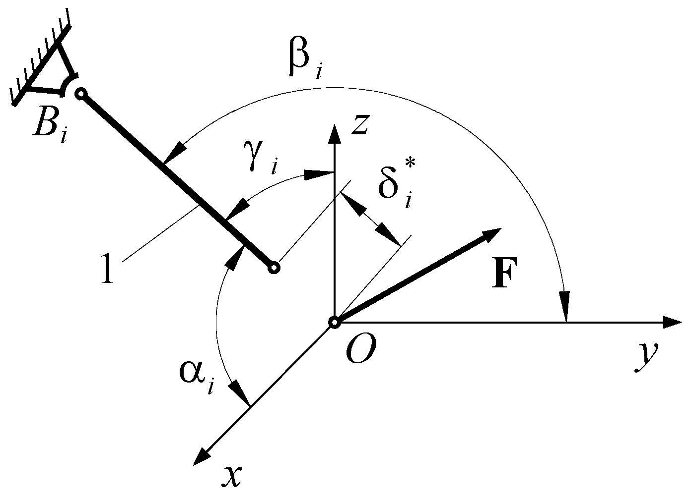
2. Mathematical Model

In a previous paper [23] the authors studied the optimization of a planar systems of bars with some deviations, the bars being linked by spherical linkages at the same point. For this planar system, the authors considered a few optimizations: the displacement along a certain axis is minimum, the force in a certain bar is minimum etc. The main conclusions were that, in general, there is no single optimization point for a certain criterion. Moreover, in the planar case, some analytical calculations can be performed.

In the case of spatial bars, the problem is more complicated because it can be solved only by numerical procedures.

Let us consider a spatial system of bars, linked by spherical joint at the same point. The other extremity of each bar has a spherical linkage, too, and it can be connected to the origin $O$. The system is captured in Figure 1, where only a generic bar (bar $i$) is represented. The bar is shorter than the nominal length with the dimension ${\delta }_i^{*}$. For the nominal length of the bar, the dimension $O{B}_i$, is $l_i$. The angles between the bar and the three axes are ${\alpha }_i$ (with the $Ox$ axis), ${\beta }_i$ (with the $Oy$ axis), and ${\gamma }_i$ (with the $Oz$ axis). The point $O$ (the common point of the bars) is acted on by the force $F$ (the projections of which are $F_x$, $F_y$, and $F_z$ on the three axes). The modulus of elasticity is $E_i$, with all the bars being of circular sections of diameters $d_i$.

The action of the force $F$ (the result of the external forces that act upon the system of bars at the point $O$) leads to the displacement of the point $O$ to another point $O^{\prime }$ (not represented in figure) so that the vector $O{O}^{\prime }$ has the components $\Delta x$, $\Delta y$, and $\Delta z$ on the three axes. The new length of the bar $i$ is

$$l_i^{\prime }=\sqrt{{\left(l_i\cos {\alpha }_i+\Delta x\right)}^2+{\left(l_i\cos {\beta }_i+\Delta y\right)}^2+{\left(l_i\cos {\gamma }_i+{\Delta }_z\right)}^2}$$

(1)

Considering that $\Delta x$, $\Delta y$, and $\Delta z$ are small compared to $l_i$ such that ${\left(\Delta x\right)}^2$, ${\left(\Delta y\right)}^2$, and ${\left(\Delta z\right)}^2$ can be neglected compared to $l_i^2$, developing into a series the expression $l_i^{\prime }-l_i$ and keeping only the first term, it results in the relation

$$l_i^{\prime }\approx l_i+{\displaystyle \frac{2\left(l_i\cos {\alpha }_i+\Delta x\right)\Delta x+2\left(l_i\cos {\beta }_i+\Delta y\right)\Delta y+2\left(l_i\cos {\gamma }_i+\Delta z\right)\Delta z}{2l_i}}$$

(2)

wherefrom

$$l_i^{\prime }-l_i\approx \Delta x\cos {\alpha }_i+\Delta y\cos {\beta }_i+\Delta z\cos {\gamma }_i$$

(3)

Multiplying the previous relation by ${\displaystyle \frac{E_i{A}_i}{l_i}}$ and taking into account that $k_i={\displaystyle \frac{E_i{A}_i}{l_i}}$, we find

$$k_i\left(l_i^{\prime }-l_i\right)=k_i\cos {\alpha }_i\Delta x+k_i\cos {\beta }_i\Delta y+k_i\cos {\gamma }_i\Delta z$$

(4)

One obtains the system

$$\left\{\begin{array}{c}\left({\displaystyle \sum k_i{\cos }^2{\alpha }_i}\right)\Delta x+\left({\displaystyle \sum k_i\cos {\alpha }_i\cos {\beta }_i}\right)\Delta y+\left({\displaystyle \sum k_i\cos {\alpha }_i\cos {\gamma }_i}\right)\Delta z=F_x+{\displaystyle \sum k_i{\delta }_i^{*}\cos {\alpha }_i},\\ \left({\displaystyle \sum k_i\cos {\alpha }_i\cos {\beta }_i}\right)\Delta x+\left({\displaystyle \sum k_i{\cos }^2{\beta }_i}\right)\Delta y+\left({\displaystyle \sum k_i\cos {\beta }_i\cos {\gamma }_i}\right)\Delta z=F_y+{\displaystyle \sum k_i{\delta }_i^{*}\cos {\beta }_i},\\ \left({\displaystyle \sum k_i\cos {\alpha }_i\cos {\gamma }_i}\right)\Delta x+\left({\displaystyle \sum k_i\cos {\beta }_i\cos {\gamma }_i}\right)\Delta y+\left({\displaystyle \sum k_i{\cos }^2{\gamma }_i}\right)\Delta z=F_x+{\displaystyle \sum k_i{\delta }_i^{*}\cos {\alpha }_i}.\end{array}\right.$$

(5)

In the previous relations we have $E_i$ is the elastic (Young) modulus of the material of bar $i$, $A_i$ is the area of the cross-section of the bar $i$, while $l_i$ represents the nominal length of the bar $i$.

It is clear that the analytical optimization is an impossible task in the general case, as we shall discuss later.

3. Optimizations

Further on, we will consider that two bars are added to the existing system of bars. There are known the mechanical and geometrical parameters of the first $n$ bars (that is, one knows $k_i$, $A_i$, $l_i$, ${\delta }_i^{*}$, ${\alpha }_i$, ${\beta }_i$, and ${\gamma }_i$, $i=\overline{1, n}$). One also knows the parameters $k_{n+1}$, $k_{n+2}$, ${\delta }_{n+1}^{*}$, and ${\delta }_{n+2}^{*}$ of the two new bars and asks for the determination of the positions of the points $B_{n+1}$ and $B_{n+2}$ (that is, he or she asks for the determination of the angles ${\alpha }_{n+1}$, ${\beta }_{n+1}$, ${\gamma }_{n+1}$, ${\alpha }_{n+2}$, ${\beta }_{n+2}$, and ${\gamma }_{n+2}$). The solution is required in space.

First of all, we must observe that the angles ${\alpha }_{n+1}$, ${\beta }_{n+1}$, ${\gamma }_{n+1}$, ${\alpha }_{n+2}$, ${\beta }_{n+2}$, and ${\gamma }_{n+2}$ are not independent, because there exist the following relations

$${\cos }^2{\alpha }_{n+1}+{\cos }^2{\beta }_{n+1}+{\cos }^2{\gamma }_{n+1}=1,$$

(6)

$${\cos }^2{\alpha }_{n+2}+{\cos }^2{\beta }_{n+2}+{\cos }^2{\gamma }_{n+2}=1$$

(7)

The new system reads

$$\begin{array}{l}\left({\displaystyle \sum _{i=1}^n{k}_i{\cos }^2{\alpha }_i}+k_{n+1}{\cos }^2{\alpha }_{n+1}+k_{n+2}{\cos }^2{\alpha }_{n+2}\right)\Delta x\\ +\left({\displaystyle \sum _{i=1}^n{k}_i\cos {\alpha }_i\cos {\beta }_i}+k_{n+1}\cos {\alpha }_{n+1}\cos {\beta }_{m+1}+k_{n+2}\cos {\alpha }_{n+2}\cos {\beta }_{n+2}\right)\Delta y\\ +\left({\displaystyle \sum _{i=1}^n{k}_i\cos {\alpha }_i\cos {\gamma }_i}+k_{n+1}\cos {\alpha }_{n+1}\cos {\gamma }_{n+1}+k_{n+2}\cos {\alpha }_{n+2}\cos {\gamma }_{n+2}\right)\Delta z\\ =F_x+{\displaystyle \sum _{i=1}^n{k}_i{\delta }_i^{*}\cos {\alpha }_i}+k_{n+1}{\delta }_{n+1}^{*}\cos {\alpha }_{n+1}+k_{n+2}{\delta }_{n+2}^{*}\cos {\alpha }_{n+2} ,\end{array}$$

(8a)

$$\begin{array}{l}\left({\displaystyle \sum _{i=1}^n{k}_i\cos {\alpha }_i\cos {\beta }_i}+k_{n+1}\cos {\alpha }_{n+1}\cos {\beta }_{n+1}+k_{n+2}\cos {\alpha }_{n+2}\cos {\beta }_{n+2}\right)\Delta x\\ +\left({\displaystyle \sum _{i=1}^n{k}_i{\cos }^2{\beta }_i}+k_{n+1}{\cos }^2{\beta }_{m+1}+k_{n+2}{\cos }^2{\beta }_{n+2}\right)\Delta y\\ +\left({\displaystyle \sum _{i=1}^n{k}_i\cos {\beta }_i\cos {\gamma }_i}+k_{n+1}\cos {\beta }_{n+1}\cos {\gamma }_{n+1}+k_{n+2}\cos {\alpha }_{n+2}\cos {\beta }_{n+2}\right)\Delta z\\ =F_x+{\displaystyle \sum _{i=1}^n{k}_i{\delta }_i^{*}\cos {\beta }_i}+k_{n+1}{\delta }_{n+1}^{*}\cos {\beta }_{n+1}+k_{n+2}{\delta }_{n+2}^{*}\cos {\beta }_{n+2} ,\end{array}$$

(8b)

$$\begin{array}{l}\left({\displaystyle \sum _{i=1}^n{k}_i\cos {\alpha }_i\cos {\gamma }_i}+k_{n+1}\cos {\alpha }_{n+1}\cos {\gamma }_{n+1}+k_{n+2}\cos {\alpha }_{n+2}\cos {\gamma }_{n+2}\right)\Delta x\\ +\left({\displaystyle \sum _{i=1}^n{k}_i\cos {\beta }_i\cos {\gamma }_i}+k_{n+1}\cos {\beta }_{n+1}\cos {\gamma }_{m+1}+k_{n+2}\cos {\beta }_{n+2}\cos {\gamma }_{n+2}\right)\Delta y\\ +\left({\displaystyle \sum _{i=1}^n{k}_i{\cos }^2{\gamma }_i}+k_{n+1}{\cos }^2{\gamma }_{n+1}+k_{n+2}{\cos }^2{\gamma }_{n+2}\right)\Delta z\\ =F_x+{\displaystyle \sum _{i=1}^n{k}_i{\delta }_i^{*}\cos {\gamma }_i}+k_{n+1}{\delta }_{n+1}^{*}\cos {\gamma }_{n+1}+k_{n+2}{\delta }_{n+2}^{*}\cos {\gamma }_{n+2}.\end{array}$$

(8c)

The tensions in the bars are

$$N_i=k_i\left(\Delta x\cos {\alpha }_i+\Delta y\cos {\beta }_i+\Delta z\cos {\gamma }_i\right)-k_i{\delta }_i^{*}$$

(9)

where $i=\overline{1, n+2}$.

Some optimizations may be realized:

(i)

the minimum displacement of the point $O$ along the $Ox$ direction; that is, one asks for the minimization of $\Delta x$;

(ii)

the minimum displacement of the point $O$ along the $Oy$ direction; that is, one asks for the minimization of $\Delta y$;

(iii)

the minimum displacement of the point $O$ along the $Oz$ direction; that is, one asks for the minimization of $\Delta z$;

(iv)

the minimum displacement of the point $O$; that is, one asks for the minimization of $\sqrt{{\left(\Delta x\right)}^2+{\left(\Delta y\right)}^2+{\left(\Delta z\right)}^2}$;

(v)

the minimum tension in a certain bar; that is, one asks for the minimization of $\left|N_i\right|$.

In all previous optimization processes, one asks for the positions of the two new bars. In these conditions, the points $B_{n+1}$ and $B_{n+2}$ (one end of each bar) are situated on certain spheres having the centers at the point $O$.

Let us discuss these optimizations. We present only the case i), the rest of them being completely similar. From system (8) it results that the displacement $\Delta x$ is a function of the angles ${\alpha }_{n+1}$. ${\beta }_{n+1}$, ${\gamma }_{n+1}$, ${\alpha }_{n+2}$, ${\beta }_{n+2}$, and ${\gamma }_{n+2}$; we write

$$\Delta x=\Delta x\left({\alpha }_{n+1},{\beta }_{n+1},{\gamma }_{n+1},{\alpha }_{n+2},{\beta }_{n+2},{\gamma }_{n+2}\right)$$

(10)

Lagrange’s function reads as

$$L=\Delta x+{\displaystyle \sum _{j=n+1}^{n+2}}{\lambda }_j\left({\cos }^2{\alpha }_j+{\cos }^2{\beta }_j+{\cos }^2{\gamma }_j-1\right)$$

(11)

and one obtains the system

$$\begin{array}{c}{\displaystyle \frac{\partial L}{\partial {\alpha }_{n+1}}}={\displaystyle \frac{\partial \Delta x}{\partial {\alpha }_{n+1}}}-2{\lambda }_{n+1}\cos {\alpha }_{n+1}\sin {\alpha }_{n+1}=-{\displaystyle \frac{\partial \Delta x}{\partial \cos {\alpha }_{n+1}}}\sin {\alpha }_{n+1}-2{\lambda }_{n+1}\cos {\alpha }_{n+1}\sin {\alpha }_{n+1}\\ =-\sin {\alpha }_{n+1}\left({\displaystyle \frac{\partial \Delta x}{\partial \cos {\alpha }_{n+1}}}+2{\lambda }_{n+1}\cos {\alpha }_{n+1}\right)=0, \dots \end{array}$$

(12)

In system (12) we have written only the first equation (corresponding for ${\alpha }_{n+1}$), the rest of them being similar.

One observes that the solutions are obtained from the non-linear system (in $\cos {\alpha }_j$, $\cos {\beta }_j$, $\cos {\gamma }_j$, ${\lambda }_{n+1}$, and ${\lambda }_{n+2}$, $j=\overline{n+1, n+2}$),

$${\displaystyle \frac{\partial \Delta x}{\partial \cos {\alpha }_{n+1}}}+2{\lambda }_{n+1}\cos {\alpha }_{n+1}=0, \dots ,$$

(13)

where, again, we wrote only the equation for ${\alpha }_{n+1}$. In fact, it is easy to see that each unknown in system (13) appears by function cosine, excepting for ${\lambda }_{n+1}$ and ${\lambda }_{n+2}$.

The system (13) is very difficult (even impossible) to be solved analytically. The only hope is the use of numerical methods. Moreover, taking into account expressions (6) and (7), the solutions of system (13) must satisfy

$$\cos {\alpha }_{n+1}\in \left[-1,1\right], \cos {\beta }_{n+1}\in \left[-1,1\right], \cos {\gamma }_{n+1}\in \left[-1,1\right],$$

(14)

$$\cos {\alpha }_{n+2}\in \left[-1,1\right], \cos {\beta }_{n+2}\in \left[-1,1\right], \cos {\gamma }_{n+2}\in \left[-1,1\right],$$

(15)

$${\cos }^2{\alpha }_{n+1}+{\cos }^2{\beta }_{n+1}\in \left[0,1\right], {\cos }^2{\alpha }_{n+2}+{\cos }^2{\beta }_{n+2}\in \left[0,1\right].$$

(16)

The reader may state that another solution of the system (12) is that given by $\sin {\alpha }_{n+1}=0$, … (again we limit ourselves to the first Equation (12)). In this case, the bar $n+1$ is in the plane $Oyz$ and the discussion is a particular one of the previous.

The reader may impose new conditions in which the ends $B_{n+1}$ or $B_{n+2}$ of the new bars may belong to different surfaces, curves etc., which can be spatial or planar ones.

It is clear that these are not the all optimizations that may be required by someone.

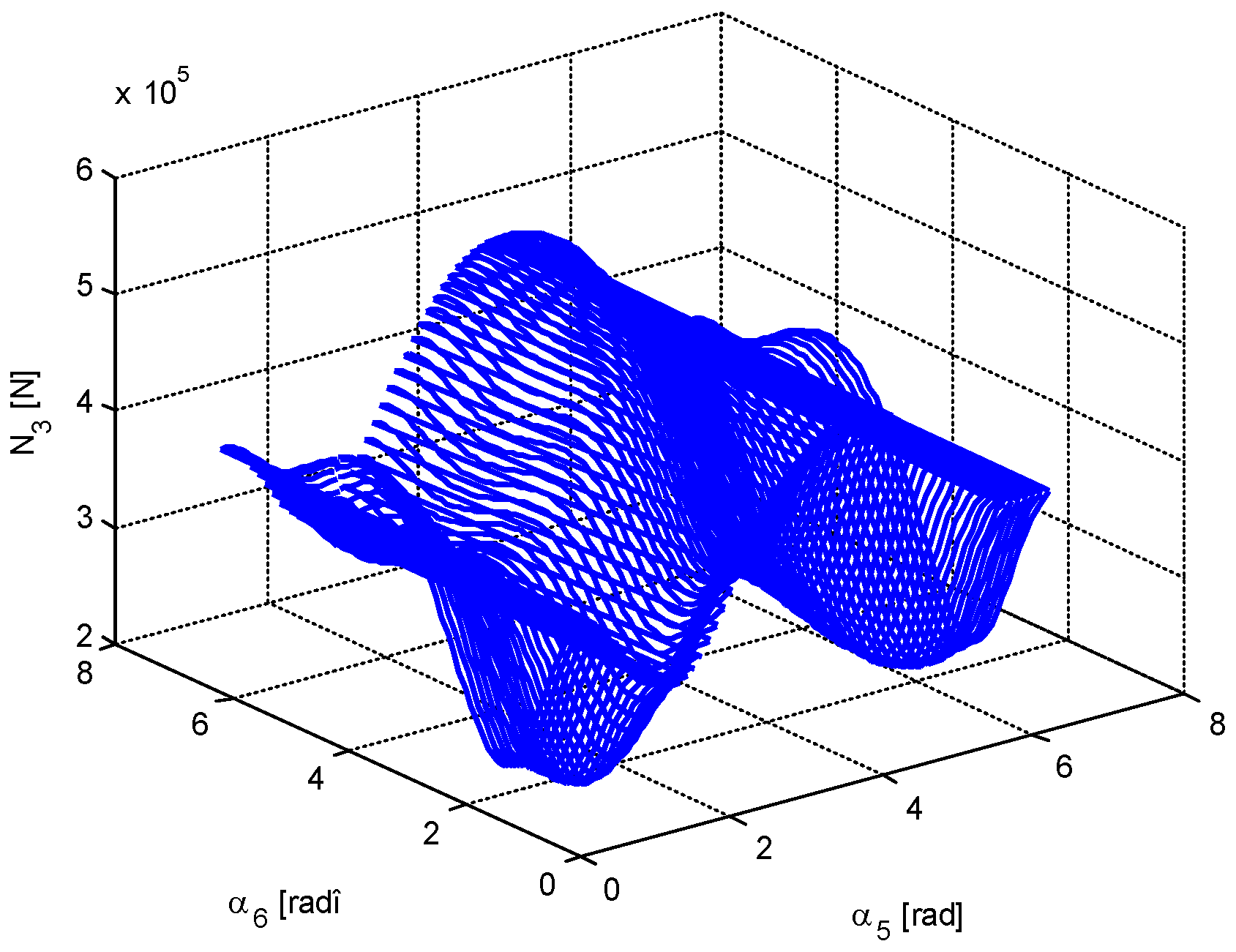
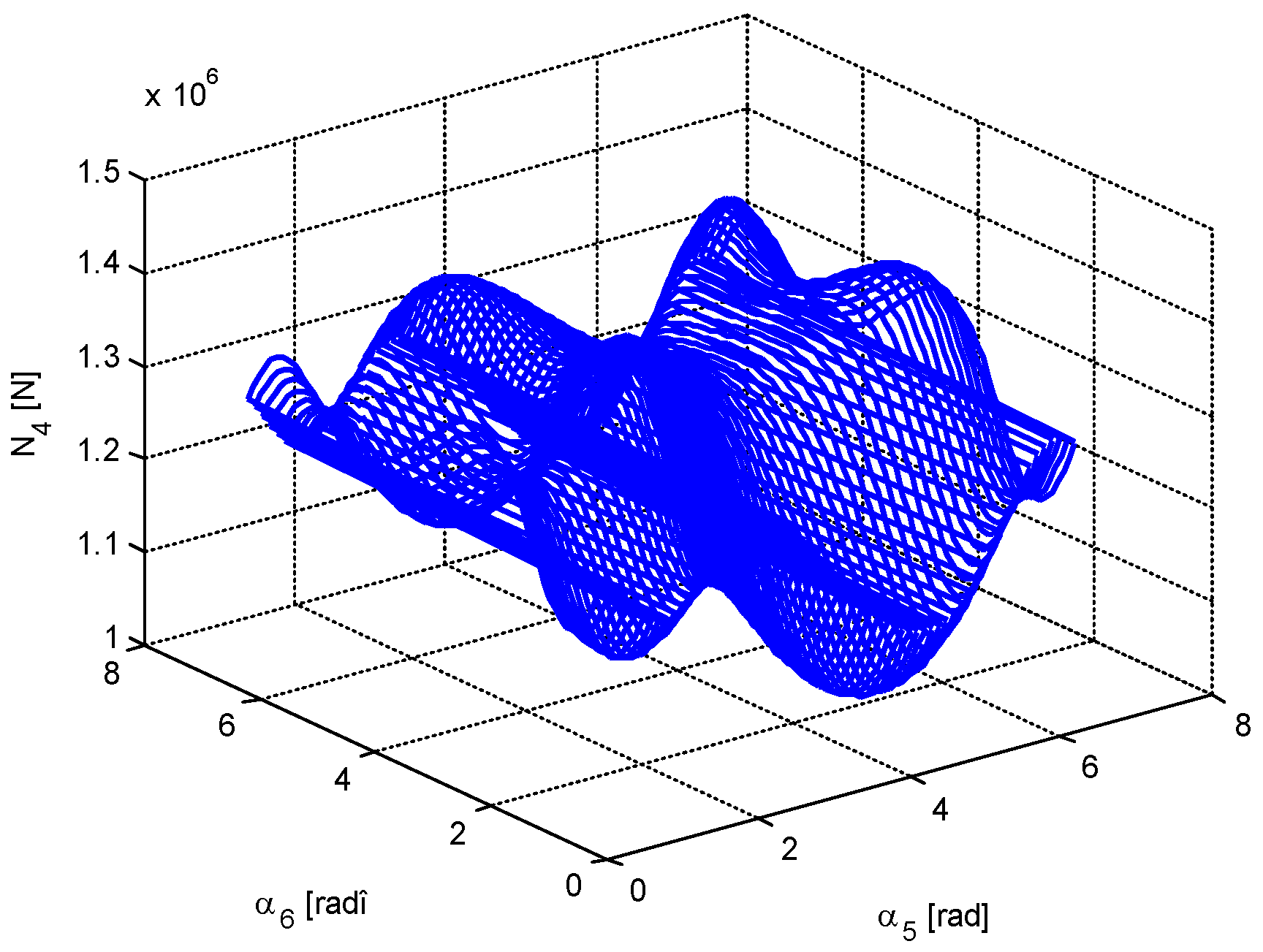
4. Numerical Simulation

We consider that the original system has four bars denoted by 1, 2, 3, and 4. The main parameters are ${\alpha }_1={\displaystyle \frac{\pi }{6}}\left[\mathrm{rad}\right]$, ${\beta }_1={\displaystyle \frac{\pi }{2}}\left[\mathrm{rad}\right]$, ${\gamma }_1=1.0471975512\left[\mathrm{rad}\right]={\displaystyle \frac{\pi }{3}}\left[\mathrm{rad}\right]$ (the angles between the first bar and the $Ox$, $Oy$, and $Oz$ axes, respectively), $E_1=2.11\times {10}^{11}\left[{\mathrm{N}/\mathrm{m}}^2\right]$ (the modulus of elasticity (Young)), $d_1=20\left[\mathrm{mm}\right]$ (the diameter of the bar), $l_1=1\left[\mathrm{m}\right]$ (the length of the bar), ${\delta }_1^{*}=2\left[\mathrm{mm}\right]$ (the bar is shorter than the nominal dimension). For the rest of the three bars we have ${\alpha }_2={\displaystyle \frac{5\pi }{3}}\left[\mathrm{rad}\right]$, ${\beta }_2={\displaystyle \frac{2\pi }{3}}\left[\mathrm{rad}\right]$, ${\gamma }_2=0.78539816341\left[\mathrm{rad}\right]={\displaystyle \frac{\pi }{4}}\left[\mathrm{rad}\right]$, $E_2=2.11\times {10}^{11}\left[{\mathrm{N}/\mathrm{m}}^2\right]$, $d_2=25\left[\mathrm{mm}\right]$, $l_2=0.9\left[\mathrm{m}\right]$, ${\delta }_2^{*}=0\left[\mathrm{mm}\right]$ (the bar has the nominal length), ${\alpha }_3={\displaystyle \frac{7\pi }{5}}\left[\mathrm{rad}\right]$, ${\beta }_3={\displaystyle \frac{11\pi }{6}}\left[\mathrm{rad}\right]$, ${\gamma }_3=1.1668221882\left[\mathrm{rad}\right]$, $E_3={10}^{11}\left[{\mathrm{N}/\mathrm{m}}^2\right]$, $d_3=40\left[\mathrm{mm}\right]$, $l_3=1.2\left[\mathrm{m}\right]$, ${\delta }_3^{*}=-1\left[\mathrm{mm}\right]$ (the bar is longer than the nominal length), ${\alpha }_4={\displaystyle \frac{\pi }{4}}\left[\mathrm{rad}\right]$, ${\beta }_4={\displaystyle \frac{\pi }{3}}\left[\mathrm{rad}\right]$, ${\gamma }_4={\displaystyle \frac{\pi }{3}}\left[\mathrm{rad}\right]$, $E_4=1.5\times {10}^{11}\left[{\mathrm{N}/\mathrm{m}}^2\right]$, $d_4=45\left[\mathrm{mm}\right]$, $l_4=0.75\left[\mathrm{m}\right]$, ${\delta }_4^{*}=0\left[\mathrm{mm}\right]$ (the bar has nominal length). Two bars (denoted by 5 and 6) are added to this system. For these bars one knows $E_5=1.5\times {10}^{11}\left[{\mathrm{N}/\mathrm{m}}^2\right]$, $d_5=18\left[\mathrm{mm}\right]$, $l_5=0.8\left[\mathrm{m}\right]$, ${\delta }_5^{*}=3\left[\mathrm{mm}\right]$ (the bar is shorter than the nominal length), and $E_6=2.3\times {10}^{11}\left[{\mathrm{N}/\mathrm{m}}^2\right]$, $d_6=15\left[\mathrm{mm}\right]$, $l_6=0.95\left[\mathrm{m}\right]$, ${\delta }_6^{*}=0\left[\mathrm{mm}\right]$ (the bar has the nominal length).

The system is acted on at the point $O$ by some forces, the result of which being $F$, with the components $F_x={10}^6\left[\mathrm{N}\right]$ (along the $Ox$ axis), $F_y=1.3\times {10}^6\left[\mathrm{N}\right]$ (along the $Oy$ axis), and $F_z=-1.5\times {10}^6\left[\mathrm{N}\right]$ (along the $Oz$ axis).

Minimization of the displacement along the $Ox$ axis leads to the value $\Delta x_{\min }\approx 0\left[\mathrm{mm}\right]$, to which two positions correspond. The first position is characterized by ${\alpha }_{51}\approx 2\left[\mathrm{rad}\right]$, ${\beta }_{51}\cong 2.6\left[\mathrm{rad}\right]$, ${\gamma }_{51}\approx 1.2617\left[\mathrm{rad}\right]$, ${\alpha }_{61}\approx 6\left[\mathrm{rad}\right]$, ${\beta }_{61}\approx 1.7\left[\mathrm{rad}\right]$, and ${\gamma }_{61}\approx 0.6548\left[\mathrm{rad}\right]$. The second position is characterized by ${\alpha }_{52}\approx 2\left[\mathrm{rad}\right]$, ${\beta }_{52}\cong 2.6\left[\mathrm{rad}\right]$, ${\gamma }_{52}\approx 1.2617\left[\mathrm{rad}\right]$, ${\alpha }_{62}\approx 6\left[\mathrm{rad}\right]$, ${\beta }_{62}\approx 1.7\left[\mathrm{rad}\right]$, and ${\gamma }_{62}\approx -0.6548\left[\mathrm{rad}\right]$. In both situations $\Delta y\approx 2.177\left[\mathrm{mm}\right]$, and $\Delta z\approx 4.743\left[\mathrm{mm}\right]$. The forces in the bars are (in both situations) $N_1\approx \mathrm{24,502.9}\left[\mathrm{N}\right]$, $N_2\approx \mathrm{259,451}\left[\mathrm{N}\right]$, $N_3\approx \mathrm{497,372.9}\left[\mathrm{N}\right]$, $N_4\approx \mathrm{1,100,537.3}\left[\mathrm{N}\right]$, $N_5\approx -\mathrm{195,953.5}\left[\mathrm{N}\right]$, $N_6=\mathrm{148,940.9}\left[\mathrm{N}\right]$ (only the force $N_5$ is a compression one). We also obtain $\Delta y_{\min }\approx 0.984\left[\mathrm{mm}\right]$ (minimization for the displacement along the $Oy$ axis) for two positions; $\Delta z_{\min }\approx 0.249\left[\mathrm{mm}\right]$ (minimization of the displacement along the $Oz$ axis also for two positions; ${\Delta }_{\min }\approx 3.498\left[\mathrm{mm}\right]$ (minimization of the global displacement $\Delta =\sqrt{{\left(\Delta x\right)}^2+{\left(\Delta y\right)}^2+{\left(\Delta z\right)}^2}$), for three positions; $\left|N_{1\min }\right|\approx 0.412936\left[\mathrm{N}\right]$ (minimization of the absolute value of the force in bar 1), for four positions; $\left|N_{2\min }\right|\approx \mathrm{24,879.363383}\left[\mathrm{N}\right]$ (minimization of the absolute value of the force in bar 2), for two positions; $\left|N_{3\min }\right|\approx \mathrm{198,883.59026}\left[\mathrm{N}\right]$ (minimization of the absolute value of the force in bar 3), for two positions; $\left|N_{4\min }\right|\approx \mathrm{966,766.4566}\left[\mathrm{N}\right]$ (minimization of the absolute value of the force in bar 4), for four positions; $\left|N_{5\min }\right|\approx 0.001777\left[\mathrm{N}\right]$ (minimization of the absolute value of the force in bar 5), two positions; $\left|N_{6\min }\right|\approx 0.006316\left[\mathrm{N}\right]$ (minimization of the absolute value of the force in bar 6), for one position.

The reader may conclude:

-

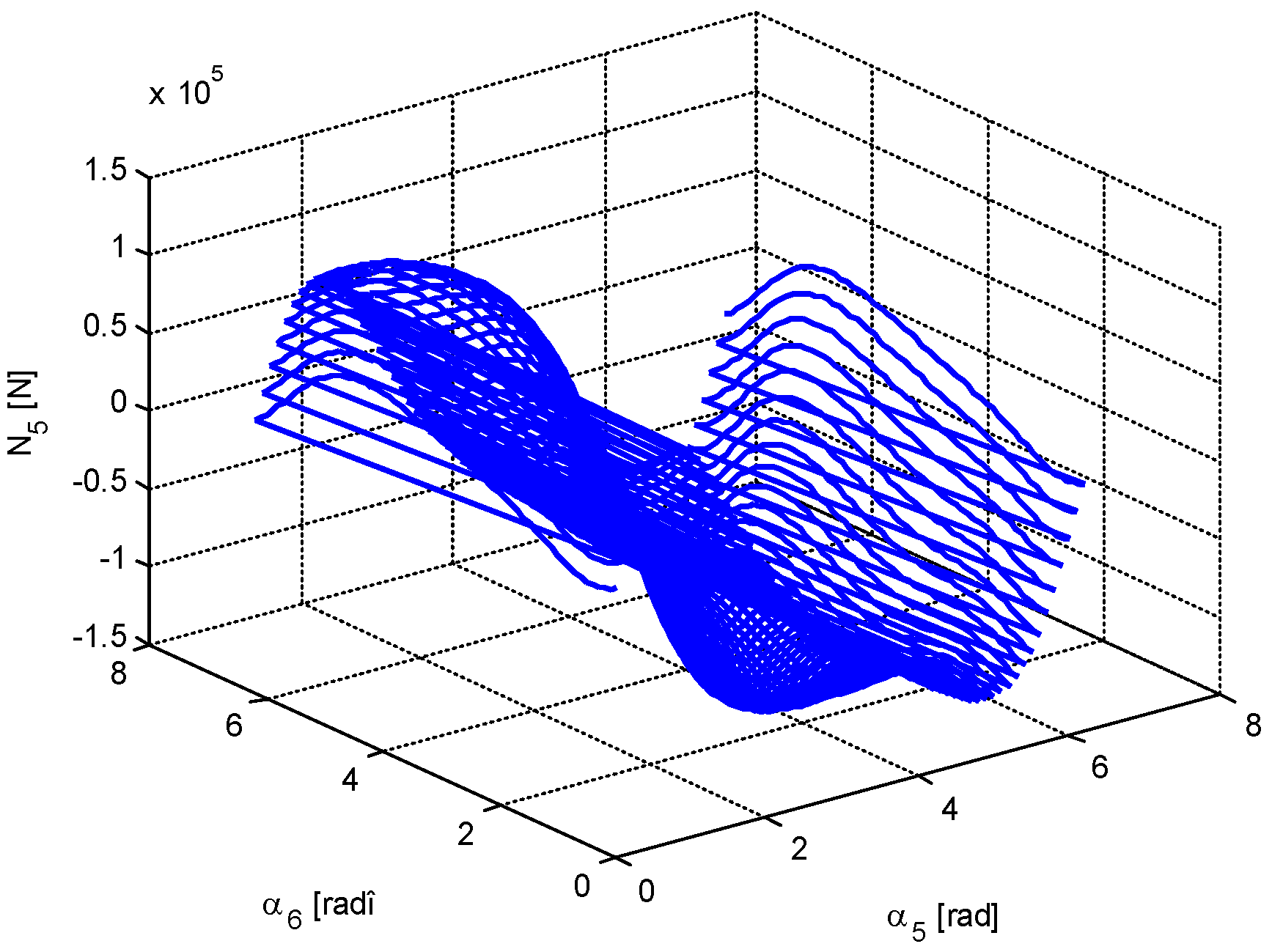
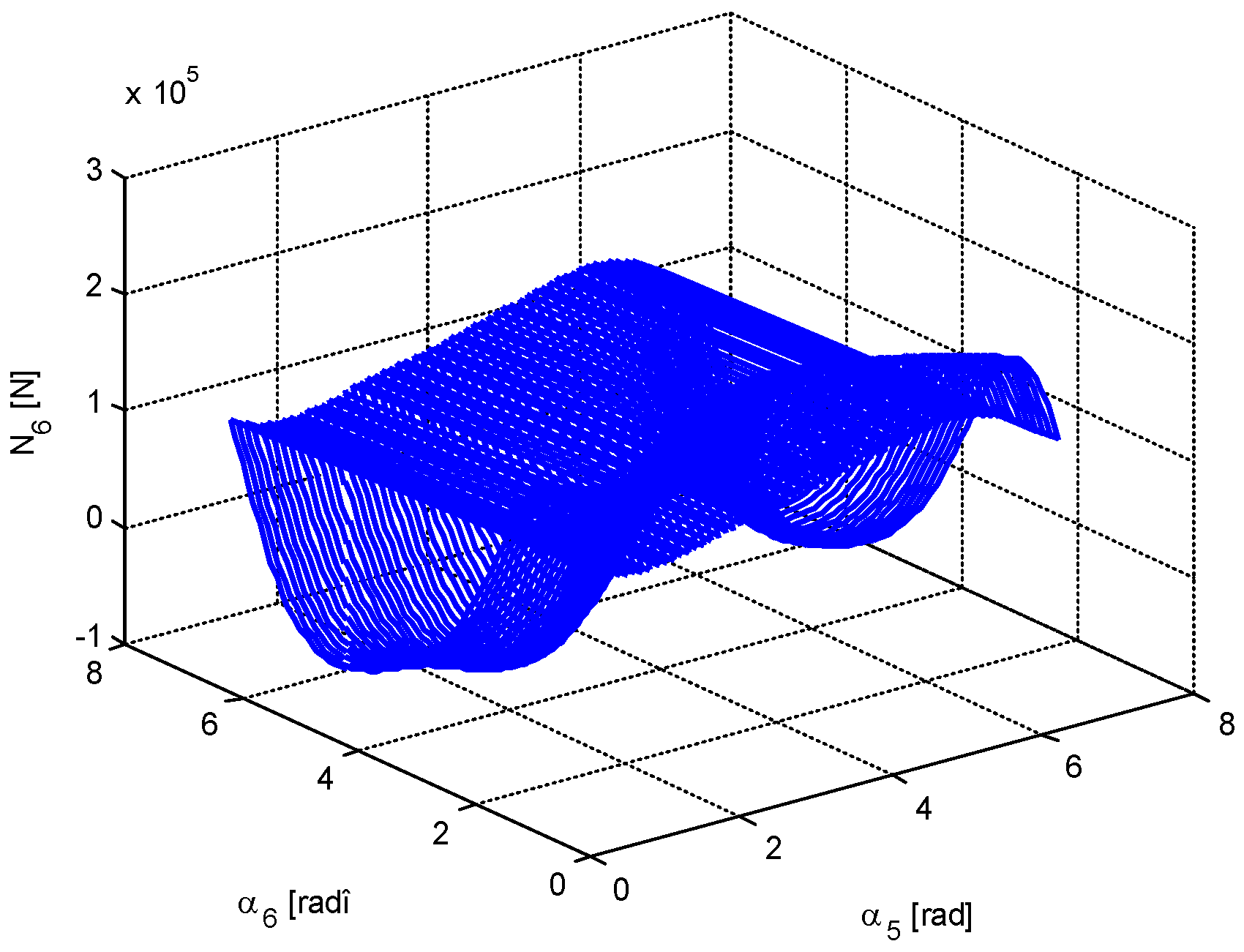
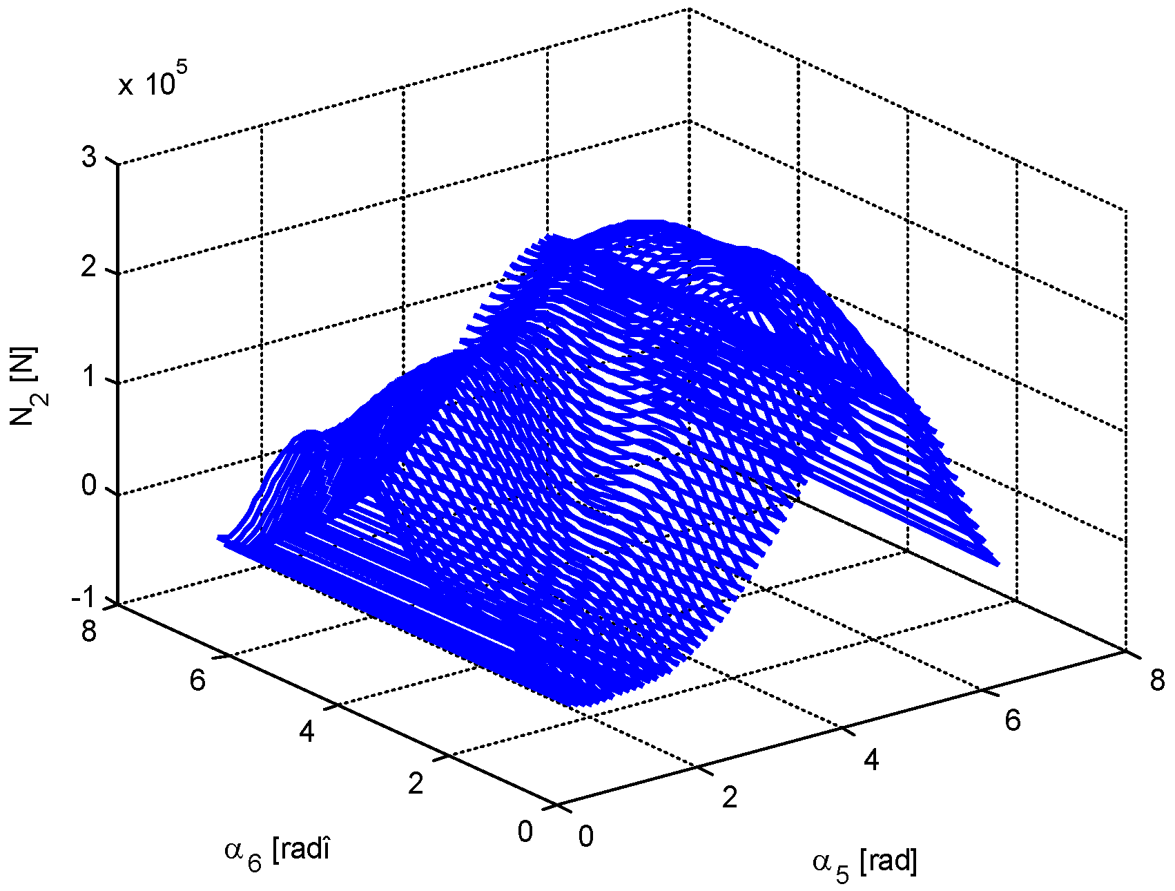
The minimum value of the force in bar 5 is very close to 0; that is, there are two positions in which the bar 5 is useless. The same conclusion, but for one position, is valid for bar 6.

-

It is possible to obtain a very small value for the force in bar 1; that is, in a certain configuration, bar 1 may be eliminated.

-

There are not equal numbers of positions for which different parameters are minimized (there are one, two, three, or four positions of minimum value for a certain parameter).

-

Based on a certain criterion, one obtains some values for the optimization parameters, values which do not coincide to those obtained using another optimization criterion.

The problem can be simplified by imposing some additional requirements for bars 5 and 6. For instance, one may keep the same parameters as in previous example but he or she may impose the supplementary conditions ${\gamma }_5=0$, and ${\gamma }_6=0$; that is, the ends $A_5$ and $A_6$ of the bars 5 and 6, respectively, are situated in the plane $Oxy$. In this situation, only the angles ${\alpha }_5$ and ${\alpha }_6$ are sufficient for the determination of the positions of the two bars. In this situation, some spatial diagrams may be presented (Figure 2, Figure 3, Figure 4, Figure 5, Figure 6, Figure 7, Figure 8, Figure 9 and Figure 10).

The minimum and maximum values are obtained as follows: $\Delta x_{\min }\approx 0.392\left[\mathrm{mm}\right]$ (one position for ${\alpha }_5\approx 4\left[\mathrm{rad}\right]$ and ${\alpha }_6\approx 0\left[\mathrm{rad}\right]$), $\Delta y_{\min }\approx 1.431\left[\mathrm{mm}\right]$ (one position), $\Delta z_{\min }\approx -0.386\left[\mathrm{mm}\right]$, $N_{1\min }\approx \mathrm{14,304.9}\left[\mathrm{N}\right]$, $N_{2\min }\approx -\mathrm{16,586.8}\left[\mathrm{N}\right]$, $N_{3\min }\approx \mathrm{214,801.6}\left[\mathrm{N}\right]$, $N_{4\min }\approx \mathrm{1,066,146}.8\left[\mathrm{N}\right]$, $N_{5\min }\approx -\mathrm{141,862.9}\left[\mathrm{N}\right]$, $N_{6\min }\approx -\mathrm{50,939.2}\left[\mathrm{N}\right]$; $\Delta x_{\max }\approx 4.102\left[\mathrm{mm}\right]$, $\Delta y_{\max }\approx 3.855\left[\mathrm{mm}\right]$, $\Delta z_{\max }\approx 4.106\left[\mathrm{mm}\right]$, $N_{1\max }\approx \mathrm{114,135.2}\left[\mathrm{N}\right]$, $N_{2\max }\approx \mathrm{281,681.1}\left[\mathrm{N}\right]$, $N_{3\max }\approx \mathrm{535,152.7}\left[\mathrm{N}\right]$, $N_{4\max }\approx \mathrm{1,440,956.5}\left[\mathrm{N}\right]$, $N_{5\max }\approx \mathrm{147,041.5}\left[\mathrm{N}\right]$, $N_{6\max }\approx \mathrm{235,745.7}\left[\mathrm{N}\right]$. Each extremum is obtained at one position.

One may state:

-

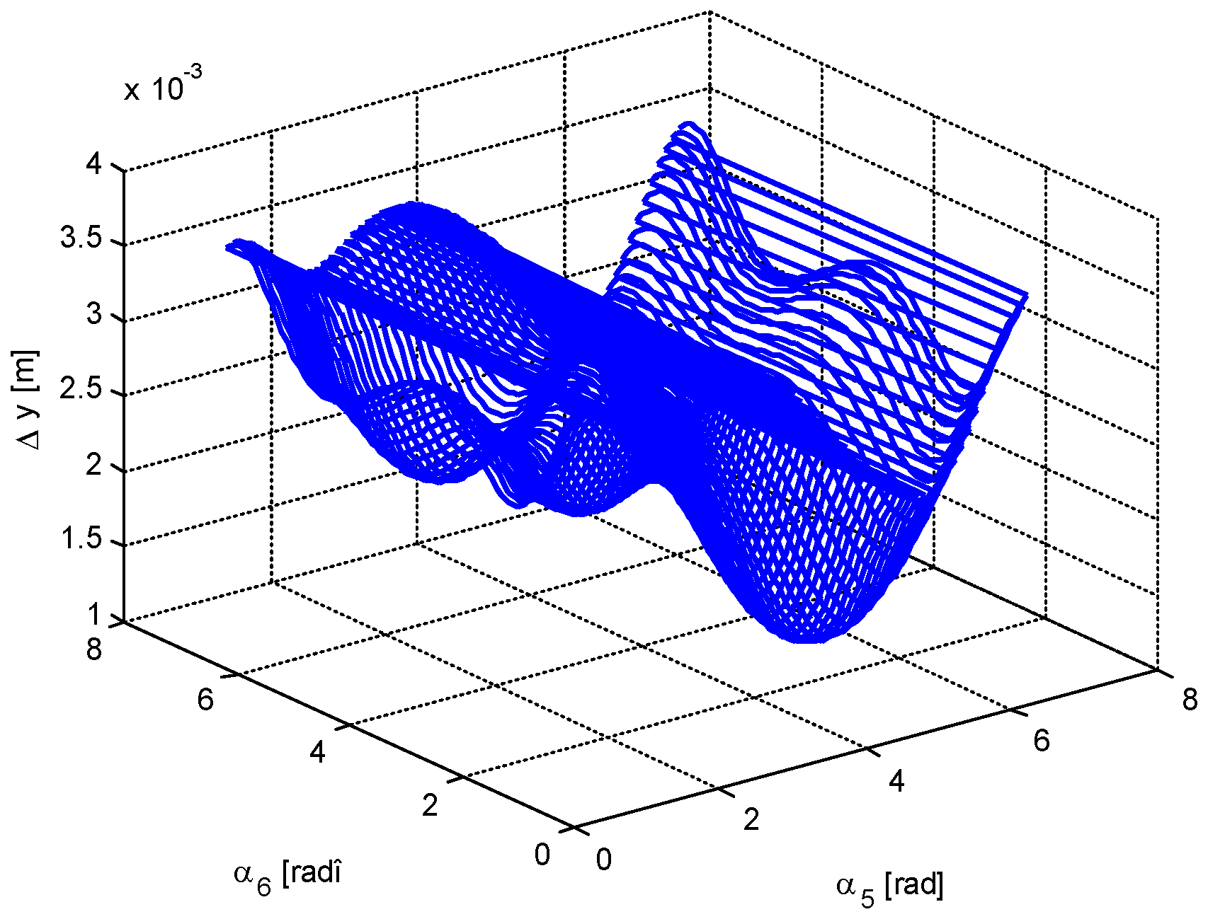
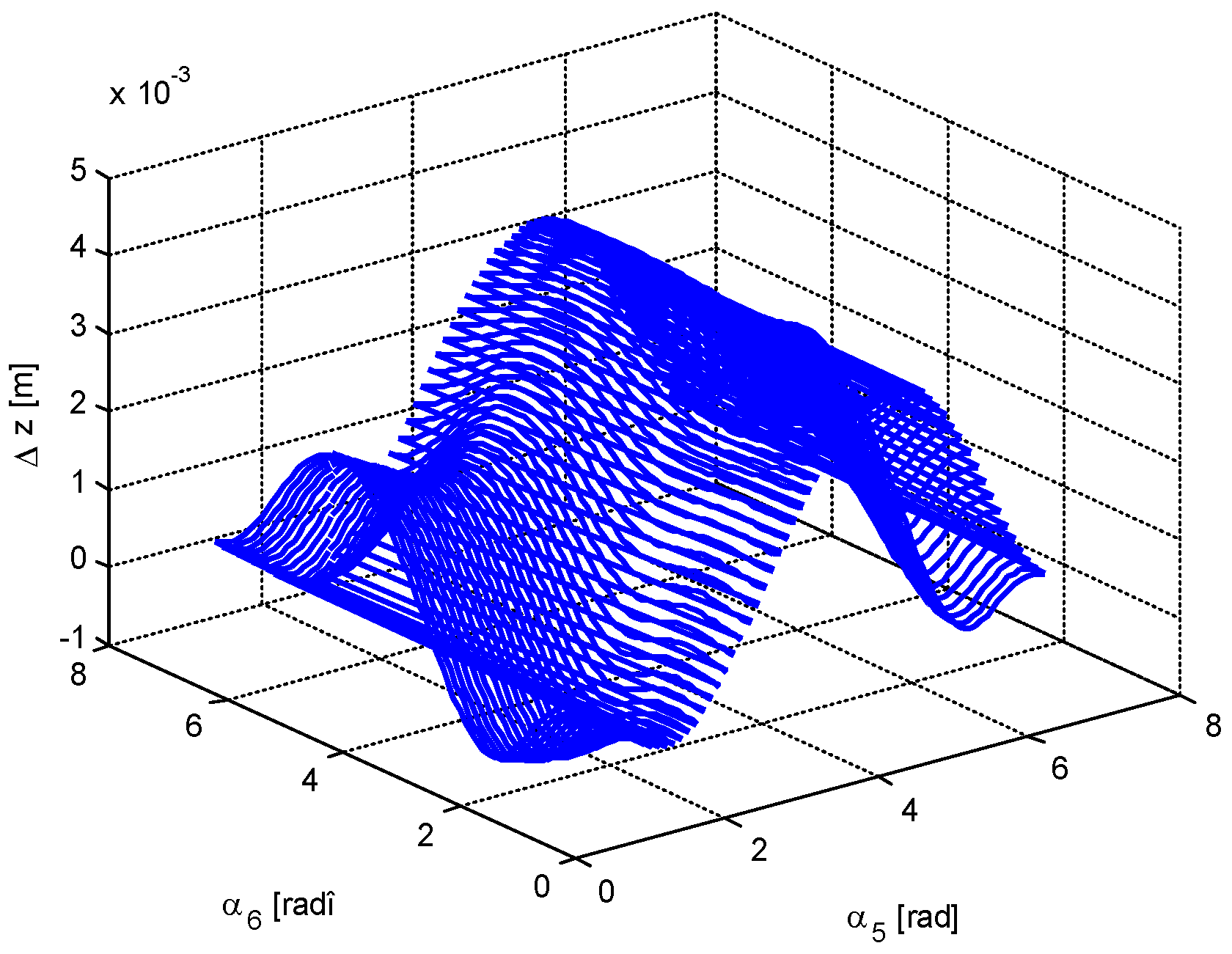
The displacements may be positive or negative. There is no rule to determine the sign of a certain displacement.

-

The forces in the bars may be also positive and negative and, again, there is no rule for the determination of the sign.

-

Generally speaking, the diagrams of variation for different parameters cannot be obtained by analytical calculation.

-

The calculation is valid only for small deformations of the bars (the statement holds true for the cases considered in this paper).

A practical problem is that of a chandelier. It is suspended by bars or chains and the addition of bars or chains is required so that certain requirements are met. If we only have chains, then all the forces in them must be positive (chains cannot be subjected to compression). It is possible that the new bars or chains cannot be connected to the walls or ceiling except in certain areas. Other restrictions can be thought of, too.

5. Conclusions

In our paper we described a method from which one may determine the displacements of the point of concurrence of bars (in our study it was the origin of the system) and the forces in bars for a system of spatial bars. The bars have at their ends spherical linkages and it results that only longitudinal forces may appear in each bar.

The method purposed in this paper can be used for any configuration of bars. The method is based on screw coordinates and can be applied for a small deformation of the bars. Practically, it is very difficult to state if the method can be applied to a certain system. One has to carry out some calculations to determine the deformations of the bars and to decide if the method can be applied. Some bars may be longer or shorter than their nominal lengths.

The method is simple and leads to a linear system of equations from which one can determine the components of the deviation of the origin (if one asks only for the deviation (or certain component/components) of the deviation). The problem becomes more complicated when the positions of certain bars are unknown and one asks for some criterion of optimization.

The optimization becomes more difficult if one considers more than two bars for which the positions of one of their ends are unknown. As we have seen, the obtained system is a non-linear one. The convergence to one solution (of an initial approximation of that solution) is assured if the initial approximation is close enough to the exact solution; that is, one has to know a relatively small vicinity of the solution.

In our future work we will consider that at the ends of the bars there exist arbitrary joints. This case is more complicated because in each point of an arbitrary bar may exist six different components (three forces and three moments).

References

1. Răcășan, V.; Pandrea, N.; Stănescu, N.-D. On the rigid hung by elastic bars subjected to axial forces. In Proceedings of the 29th International Congress on Sound and Vibration, Prague, Czech Republic, 9–13 July 2023. [Google Scholar]
2. Hwang, Y.-L. Dynamic recursive decoupling method for closed-loop flexible mechanical systems. Int. J. Non-Linear Mech. 2006, 41, 1181–1190. [Google Scholar] [CrossRef]
3. Marques, F.; Roupa, I.; Silva, M.T.; Flores, P.; Lankarani, H.M. Examination and comparison of different methods to model closed loop kinematic chains using Lagrangian formulation with cut joint, clearance joint constraint and elastic joint approaches. Mech. Mach. Theory 2021, 160, 104294. [Google Scholar] [CrossRef]
4. Sorgonà, O.; Cirelli, M.; Giannini, O.; Verotti, M. Comparison of flexibility models for the multibody simulation of compliant mechanisms. Multibody Syst. Dyn. 2024; online. [Google Scholar]
5. Chen, J.; Chen, Q.; Liang, D.; Mo, J. Solution of geometrico-static problems and motion experiments for a suspended under-constrained parallel mechanism driven by two flexible cables. J. Mech. Sci. Technol. 2024, 38, 4365–4376. [Google Scholar] [CrossRef]
6. Gallardo-Alvarado, J. Jerk distribution of a 6-3 Gough-Stewart platform. Proc. Inst. Mech. Eng. Part K J. Multi-Body Dyn. 2013, 217, 77–84. [Google Scholar] [CrossRef]
7. Zhou, H.; Cao, Y.; Li, B.; Wu, M.; Yu, J.; Chen, H. Position-Singularity Analysis of a Class of the 3/6-Gough-Stewart Manipulators based on Singularity-Equivalent-Mechanism. Int. J. Adv. Robot. Syst. 2012, 9, 1–9. [Google Scholar] [CrossRef]
8. Ding, X.; Isaksson, M. Quantitative analysis of decoupling and spatial isotropy of a generalised rotation-symmetric 6-DOF Stewart platform. Mech. Mach. Theory 2023, 180, 105156. [Google Scholar] [CrossRef]
9. Šika, Z.; Krivošej, J.; Vyhlídal, T. Three dimensional delayed resonator of Stewart platform type for entire absorption of fully spatial vibration. J. Sound Vib. 2024, 571, 118154. [Google Scholar] [CrossRef]
10. Hajimirzaallan, H.; Ferraresi, C.; Moosavi, H.; Massah, M. An analytical method for the inverse dynamic analysis of the Stewart platform with asymmetric-adjustable payload. Proc. Int. Inst. Mech. Eng. Part K J. Multi-Body Dyn. 2013, 227, 162–171. [Google Scholar] [CrossRef]
11. Leonov, G.A.; Zegzhda, S.A.; Zuev, S.M.; Ershov, B.A.; Kazunin, D.V.; Kostygova, D.M.; Kuznetsov, N.V.; Tovstik, P.E.; Tovstik, T.P.; Yushkov, M.P. Dynamics and Control of the Stewart platform. Dokl. Phys. 2014, 59, 405–410. [Google Scholar] [CrossRef]
12. Korkealaakso, P.; Mikkola, A.; Rantalainen, T.; Rouvinen, A. Description of joint constraints in the floating frame of reference formulation. Proc. Inst. Mech. Eng. Part K J. Multi-Body Dyn. 2009, 223, 133–145. [Google Scholar] [CrossRef]
13. Bouzgarrou, B.C.; Ray, P.; Gogu, G. New approach for dynamic modeling of flexible manipulators. Proc. Inst. Mech. Eng. Part K J. Multi-Body Dyn. 2005, 219, 285–298. [Google Scholar]
14. Huang, Z.; Zhao, Y.; Liu, J. Kinetostatic Analysis of 4-R (CRR) Parallel Manipulator with Overconstraints via Reciprocal-Screw Theory. Adv. Mech. Eng. 2010, 2, 404960. [Google Scholar] [CrossRef]
15. Stan, A.-F.; Pandrea, N.; Stănescu, N.-D.; Munteanu, L.; Chiroiu, V. On the vibrations of a Rigid Solid Hung by Kinematic Chains. Symmetry 2022, 14, 770. [Google Scholar] [CrossRef]
16. Hu, Y.; Zhang, H.; Wang, K.; Fang, Y.; Ma, C. Analytical analysis of vibration isolation characteristics of quasi-zero stiffness suspension backpack. Int. J. Dyn. Control, 2024; online. [Google Scholar]
17. Chen, W.; Wang, S.; Li, J.; Lin, C.; Yang, Y.; Ren, A.; Li, W.; Zhao, X.; Zhang, W.; Guo, W.; et al. An ADRC-based triple-loop control strategy of ship-mounted Stewart platform for six-DOF wave compensation. Mech. Mach. Theory 2023, 184, 105289. [Google Scholar] [CrossRef]
18. Yang, S.; Xu, P.; Li, B. Design and rigid-flexible dynamic analysis of a morphing wing eight-bar mechanism. Nonlinear Dyn. 2024, 112, 15025–15060. [Google Scholar] [CrossRef]
19. Chen, G.; Rui, X.; Abbas, L.K.; Wang, G.; Yang, F.; Zhu, W. A novel method for the dynamic modeling of Stewart parallel mechanism. Mech. Mach. Theory 2018, 126, 397–412. [Google Scholar] [CrossRef]
20. Xu, A.; Xu, Z.; Zhang, H.; He, S.; Wang, L. Novel coarse and fine stage parallel vibration isolation pointing platform for space optics payload. Mech. Syst. Signal Process. 2024, 213, 111359. [Google Scholar] [CrossRef]
21. Jiang, Y.; Xiao, H.; Yang, G.; Guo, H.; Liu, R.; Deng, Z. Study on transient dynamics of the pyrotechnic-driven large flexible expansion mechanism. Nonlinear Dyn. 2024, 112, 15917–15932. [Google Scholar] [CrossRef]
22. Pandrea, N. Elements of Mechanics of Rigid Solids in Plűckerian Coordinates; The Romanian Academy Publishing House: Bucharest, Romania, 2000. [Google Scholar]
23. Răcășan, V.; Stănescu, N.-D. Minimization of the small deformations for a planar system of concurrent bars jointed at their ends. In Proceedings of the 30th International Congress on Sound and Vibration, Amsterdam, The Netherlands, 8–11 July 2024. [Google Scholar]
Figure 1. Mathematical model.
Mathematics 12 02680 g001
Figure 2. Diagram Δ x = Δ x α 5 , α 6 for α 5 0 ,   2 π , α 6 0 ,   2 π .
Mathematics 12 02680 g002
Figure 3. Diagram Δ y = Δ y α 5 , α 6 for α 5 0 ,   2 π , α 6 0 ,   2 π .
Mathematics 12 02680 g003
Figure 4. Diagram Δ z = Δ z α 5 , α 6 for α 5 0 ,   2 π , α 6 0 ,   2 π .
Mathematics 12 02680 g004
Figure 5. Diagram N 1 = N 1 α 5 , α 6 for α 5 0 ,   2 π , α 6 0 ,   2 π .
Mathematics 12 02680 g005
Figure 6. Diagram N 21 = N 2 α 5 , α 6 for α 5 0 ,   2 π , α 6 0 ,   2 π .
Mathematics 12 02680 g006
Figure 7. Diagram N 3 = N 3 α 5 , α 6 for α 5 0 ,   2 π , α 6 0 ,   2 π .
Mathematics 12 02680 g007
Figure 8. Diagram N 4 = N 4 α 5 , α 6 for α 5 0 ,   2 π , α 6 0 ,   2 π .
Mathematics 12 02680 g008
Figure 9. Diagram N 5 = N 5 α 5 , α 6 for α 5 0 ,   2 π , α 6 0 ,   2 π .
Mathematics 12 02680 g009
Figure 10. Diagram N 6 = N 6 α 5 , α 6 for α 5 0 ,   2 π , α 6 0 ,   2 π .
Mathematics 12 02680 g010
Disclaimer/Publisher’s Note: The statements, opinions and data contained in all publications are solely those of the individual author(s) and contributor(s) and not of MDPI and/or the editor(s). MDPI and/or the editor(s) disclaim responsibility for any injury to people or property resulting from any ideas, methods, instructions or products referred to in the content.