
Dynamics of Activation and Regulation of the Immune Response to Attack by Viral Pathogens Using Mathematical Modeling
 , , , and
Abstract
:1. Introduction
2. Methods
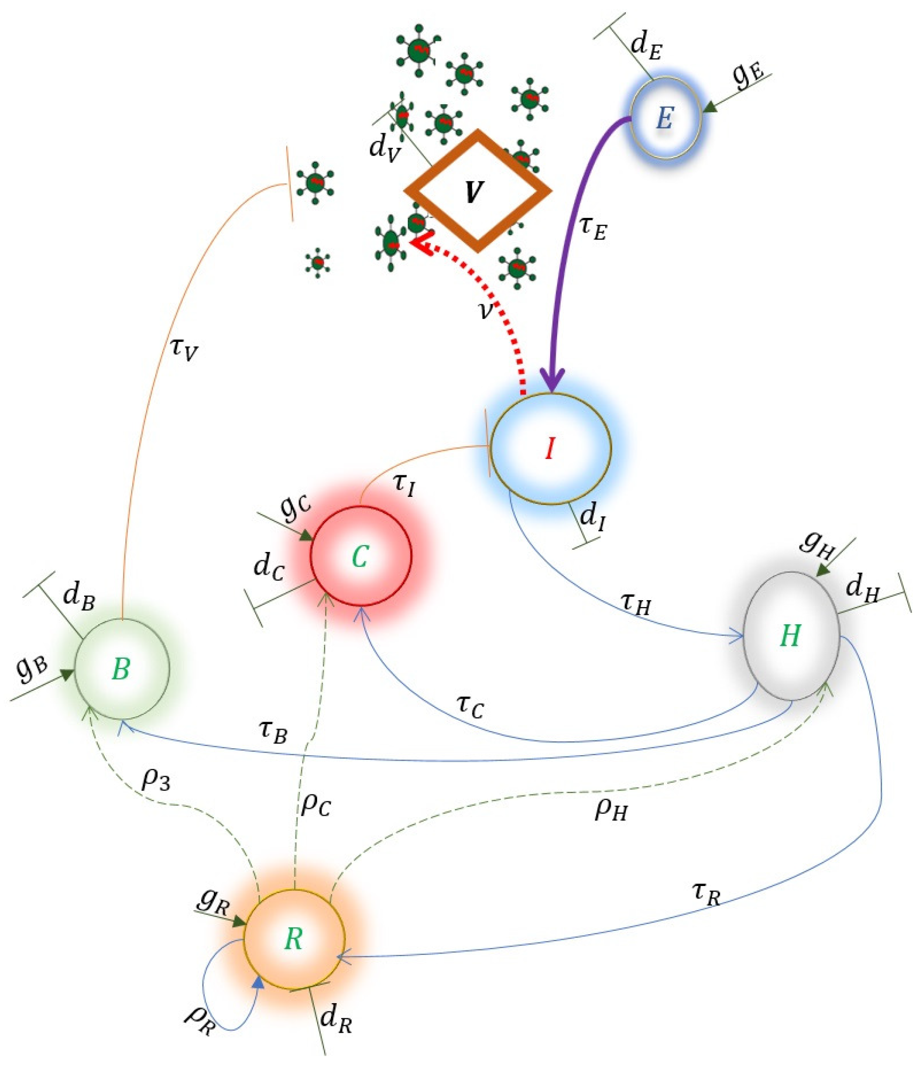
Model
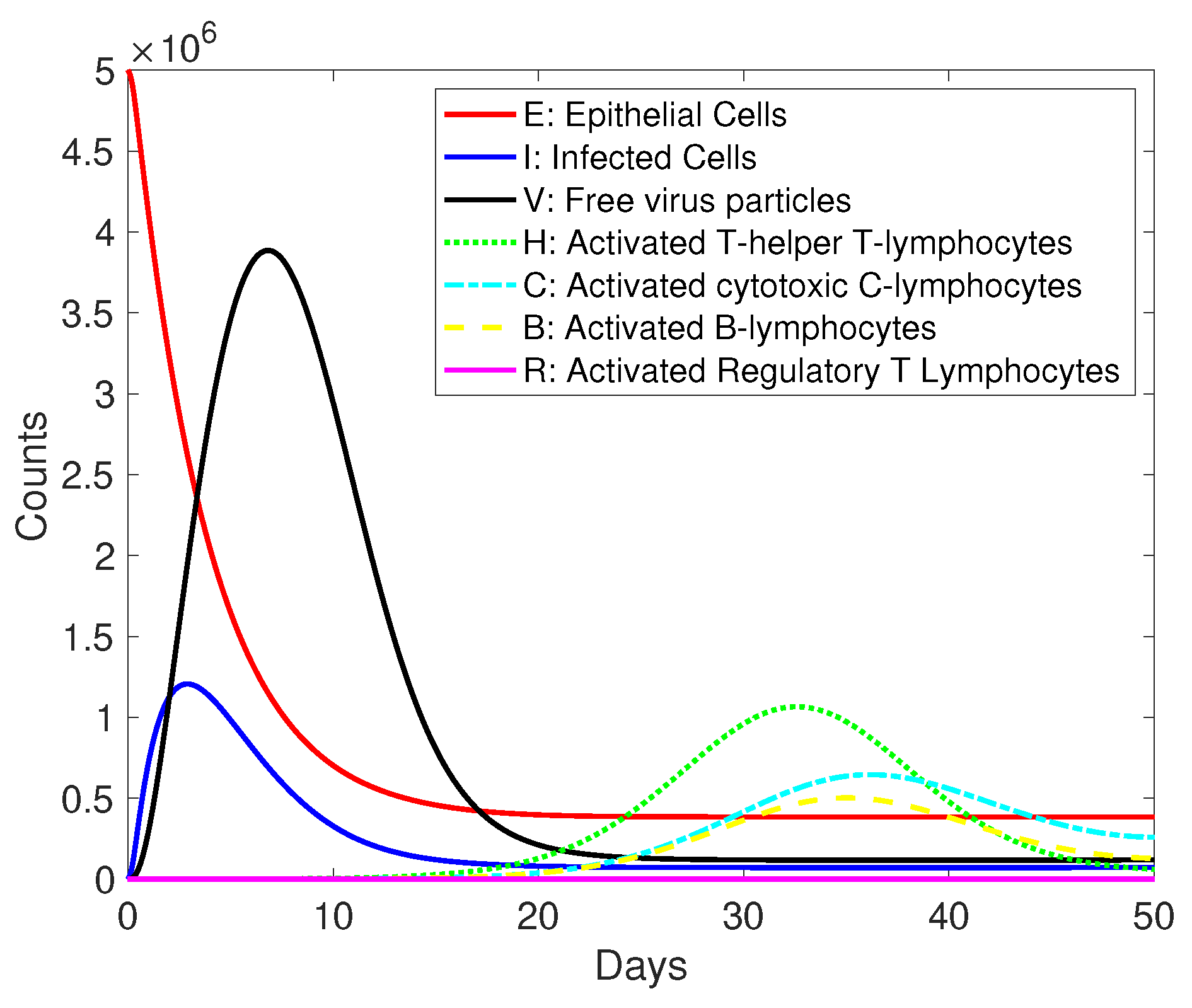
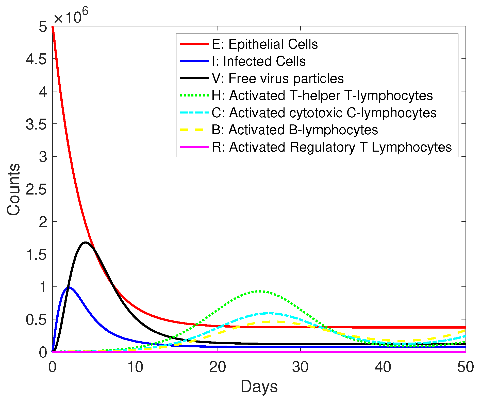
- Helper and cytotoxic T lymphocytes and B lymphocytes curves do not achieve a sufficiently rapid decline in the simulations. In the immune response to infection, there is a more rapid decline in the number of active lymphocytes after antigen clearance is achieved.
- There is an over-dependence on cell turnover parameters and . It is not possible to adjust cell turnover parameters to achieve a further decline in lymphocyte populations after infection. We have the restriction that and do not exceed deaths to avoid explosive growth.
3. Results and Discussion
Basic Reproductive Number
4. Conclusions
Author Contributions
Funding
Data Availability Statement
Acknowledgments
Conflicts of Interest
Appendix A. Positivity of a Homogeneous System
- if for all and
- if for all .
Appendix B. Positivity of a Non-Homogeneous System
- Case 1: for all . In addition, for all . From the first equation of the Cauchy problem above, we have . We have a contradiction, and such a case is impossible.
- Case 2: for all . In addition, for all . From the second equation of the Cauchy problem above, we have . We again have a contradiction, and such a case is also impossible.
Appendix C. Stability
References
- Pincheira-Brown, P.; Bentancor, A. Forecasting COVID-19 infections with the semi-unrestricted generalized growth model. Epidemics. 2021, 37, 100486. [Google Scholar] [CrossRef] [PubMed]
- Wang, S.; Pan, Y.; Wang, Q.; Miao, H.; Brown, A.N.; Rong, L. Modeling the viral dynamics of SARS-CoV-2 infection. Math. Biosci. 2020, 328, 108438. [Google Scholar] [CrossRef] [PubMed]
- Du, S.Q.; Yuan, W. Mathematical modeling of interaction between innate and adaptive immune responses in COVID-19 and implications for viral pathogenesis. J. Med. Virol. 2020, 92, 1615–1628. [Google Scholar] [CrossRef] [PubMed]
- Vetter, P.; Eberhardt, C.S.; Meyer, B.; Martinez Murillo, P.A.; Torriani, G.; Pigny, F.; Lemeille, S.; Cordey, S.; Laubscher, F.; Vu, D.-L.; et al. Daily viral kinetics and innate and adaptive immune response assessment in COVID-19: A case series. mSphere 2020, 5, e00827-20. [Google Scholar] [CrossRef] [PubMed]
- Kamae, I. A theory of diagnostic testing to stop the virus spreading: Evidence-based reasoning to resolve the COVID-19 crisis by testing. Keio J. Med. 2022, 71, 13–20. [Google Scholar] [CrossRef]
- Pal, M.; Berhanu, G.; Desalegn, C.; Kandi, V. Severe acute respiratory syndrome coronavirus-2 (SARS-CoV-2): An update. Cureus 2020, 12, e7423. [Google Scholar] [CrossRef]
- Abduljalil, J.M.; Abduljalil, B.M. Epidemiology, genome, and clinical features of the pandemic SARS-CoV-2: A recent view. New Microbes New Infect. 2020, 35, 100672. [Google Scholar] [CrossRef]
- Larsen, J.R.; Martin, M.R.; Martin, J.D.; Hicks, J.B.; Kuhn, P. Modeling the onset of symptoms of COVID-19: Effects of SARS-CoV-2 variant. PLoS Comput. Biol. 2021, 17, e1009629. [Google Scholar] [CrossRef]
- Chen, J.; Wang, R.; Wang, M.; Wei, G.-W. Mutations strengthened SARS-CoV-2 infectivity. J. Mol. Biol. 2020, 432, 5212–5226. [Google Scholar] [CrossRef]
- Layton, A.T.; Sadria, M. Understanding the dynamics of SARS-CoV-2 variants of concern in ontario, canada: A modeling study. Sci. Rep. 2022, 12, 1–16. [Google Scholar]
- Chen, J.; Wang, R.; Gilby, N.B.; Wei, G.-W. Omicron variant (b. 1.1. 529): Infectivity, vaccine breakthrough, and antibody resistance. J. Chem. Inf. Model. 2022, 62, 412–422. [Google Scholar] [CrossRef] [PubMed]
- Kannan, S.; Ali, P.S.S.; Sheeza, A. Evolving biothreat of variant SARS-CoV-2-molecular properties, virulence and epidemiology. Eur. Rev. Med. Pharmacol. Sci. 2021, 25, 4405–4412. [Google Scholar] [PubMed]
- De, R.; Dutta, S. Role of the microbiome in the pathogenesis of COVID-19. Front. Cell. Infect. Microbiol. 2022, 12, 736397. [Google Scholar] [CrossRef] [PubMed]
- Baric, R.S. Emergence of a highly fit SARS-CoV-2 variant. N. Engl. J. Med. 2020, 383, 2684–2686. [Google Scholar] [CrossRef] [PubMed]
- Maher, M.C.; Bartha, I.; Weaver, S.; Iulio, J.D.; Ferri, E.; Leah, S.; Lempp, F.A.; Hie, B.L.; Bryson, B.; Berger, B.; et al. Predicting the mutational drivers of future SARS-CoV-2 variants of concern. Sci. Transl. Med. 2022, 14, eabk3445. [Google Scholar] [CrossRef]
- Cuesta-Herrera, L.; Córdova-Lepe, F.; Pastenes, L.; Arencibia, A.D.; Baldera-Moreno, Y.; Torres-Mantilla, H.A. A mathematical model and simulation scenarios for t and b cells immune response to severe acute respiratory syndrome-coronavirus-2. In Journal of Physics: Conference Series; IOP Publishing: Bristol, UK, 2023; Volume 2516, p. 012007. [Google Scholar]
- Kuklina, E.M. T lymphocytes as targets for SARS-CoV-2. Biochemistry 2022, 87, 566–576. [Google Scholar] [CrossRef]
- Gualana, F.L.; Maiorca, F.; Marrapodi, R.; Villani, F.; Miglionico, M.; Santini, S.A.; Pulcinelli, F.; Gragnani, L.; Piconese, S.; Fiorilli, M.; et al. Opposite effects of mrna-based and adenovirus-vectored SARS-CoV-2 vaccines on regulatory t cells: A pilot study. Biomedicines 2023, 11, 511. [Google Scholar] [CrossRef]
- Samaan, E.; Elmaria, M.O.; Khedr, D.; Gaber, T.; Elsayed, A.G.; N Shenouda, R.; Gamal, H.; Shahin, D.; Abousamra, N.K.; Shemies, R. Characterization of regulatory t cells in SARS-CoV-2 infected hemodialysis patients: Relation to clinical and radiological severity. BMC Nephrol. 2022, 23, 391. [Google Scholar] [CrossRef]
- Walter, L.O.; Cardoso, C.C.; Santos-Pirath, I.M.; Costa, H.Z.; Gartner, R.; Werle, I.; Bramorski Mohr, E.T.; da Rosa, J.S.; Lubschinski, T.L.; Felisberto, M.; et al. T cell maturation is significantly affected by SARS-CoV-2 infection. Immunology 2023, 169, 358–368. [Google Scholar] [CrossRef]
- Chaple, A.R.; Vispute, M.M.; Mahajan, S.; Mushtaq, S.; Muthuchelvan, D.; Ramakrishnan, M.A.; Kumar Sharma, G. Relational interaction between t-lymphocytes and SARS-CoV-2: A review. Acta Virol. 2021, 65, 107–114. [Google Scholar] [CrossRef]
- Gonçalves, A.; Bertrand, J.; Ke, R.; Comets, E.; Lamballerie, X.; Malvy, D.; Pizzorno, A.; Terrier, O.; Calatrava, M.R.; Mentré, F.; et al. Timing of antiviral treatment initiation is critical to reduce SARS-CoV-2 viral load. CPT Pharmacometrics Syst. Pharmacol. 2020, 9, 509–514. [Google Scholar] [CrossRef] [PubMed]
- Pawelek, K.A.; Dor, D., Jr.; Salmeron, C.; Handel, A. Within-host models of high and low pathogenic influenza virus infections: The role of macrophages. PLoS ONE 2016, 11, e0150568. [Google Scholar] [CrossRef]
- Goyal, A.; Cardozo-Ojeda, E.F.; Schiffer, J.T. Potency and timing of antiviral therapy as determinants of duration of SARS-CoV-2 shedding and intensity of inflammatory response. Sci. Adv. 2020, 6, eabc7112. [Google Scholar] [CrossRef]
- McCallum, H.; Barlow, N.; Hone, J. How should pathogen transmission be modelled? Trends Ecol. Evol. 2001, 16, 295–300. [Google Scholar] [CrossRef]
- Fischer, D.S.; Ansari, M.; Wagner, K.I.; Jarosch, S.; Huang, Y.; Mayr, C.H.; Strunz, M.; Lang, N.J.; D’Ippolito, E.; Hammel, M.; et al. Single-cell rna sequencing reveals ex vivo signatures of SARS-CoV-2-reactive t cells through ‘reverse phenotyping’. Nat. Commun. 2021, 12, 1–14. [Google Scholar] [CrossRef] [PubMed]
- He, Z.; Zhao, C.; Dong, Q.; Zhuang, H.; Song, S.; Peng, G.; Dwyer, D.E. Effects of severe acute respiratory syndrome (sars) coronavirus infection on peripheral blood lymphocytes and their subsets. Int. J. Infect. Dis. 2005, 9, 323–330. [Google Scholar] [CrossRef] [PubMed]
- Laferl, H.; Kelani, H.; Seitz, T.; Holzer, B.; Zimpernik, I.; Steinrigl, A.; Schmoll, F.; Wenisch, C.; Allerberger, F. An approach to lifting self-isolation for health care workers with prolonged shedding of SARS-CoV-2 RNA. Infection 2021, 49, 95–101. [Google Scholar] [CrossRef]
- Singanayagam, A.; Patel, M.; Charlett, A.; Bernal, J.L.; Saliba, V.; Ellis, J.; Ladhani, S.; Zambon, M.; Gopal, R. Duration of infectiousness and correlation with rt-pcr cycle threshold values in cases of COVID-19, england, january to may 2020. Eurosurveillance 2020, 25, 2001483. [Google Scholar] [CrossRef]
- Sohn, Y.; Jeong, S.J.; Chung, W.S.; Hyun, J.H.; Baek, Y.J.; Cho, Y.; Kim, J.H.; Ahn, J.Y.; Choi, J.Y.; Yeom, J.-S. Assessing viral shedding and infectivity of asymptomatic or mildly symptomatic patients with COVID-19 in a later phase. J. Clin. Med. 2020, 9, 2924. [Google Scholar] [CrossRef]
- Rhee, C.; Kanjilal, S.; Baker, M.; Klompas, M. Duration of severe acute respiratory syndrome coronavirus 2 (SARS-CoV-2) infectivity: When is it safe to discontinue isolation? Clin. Infect. Dis. 2021, 72, 1467–1474. [Google Scholar] [CrossRef]
- Challenger, J.D.; Foo, C.Y.; Wu, Y.; Yan, A.W.; Marjaneh, M.M.; Liew, F.; Thwaites, R.S.; Okell, L.C.; Cunnington, A.J. Modelling upper respiratory viral load dynamics of SARS-CoV-2. BMC Med. 2022, 20, 1–20. [Google Scholar] [CrossRef]
- Ghostine, R.; Gharamti, M.; Hassrouny, S.; Hoteit, I. Mathematical modeling of immune responses against SARS-CoV-2 using an ensemble kalman filter. Mathematics. 2021, 9, 2427. [Google Scholar] [CrossRef]
- Hattaf, K.; Yousfi, N. Dynamics of SARS-CoV-2 infection model with two modes of transmission and immune response. Math. Biosci. Eng. 2020, 17, 5326–5340. [Google Scholar] [CrossRef] [PubMed]
- Chatterjee, A.N.; Basir, F.A.; Almuqrin, M.A.; Mondal, J.; Khan, I. SARS-CoV-2 infection with lytic and non-lytic immune responses: A fractional order optimal control theoretical study. Results Phys. 2021, 26, 104260. [Google Scholar] [CrossRef] [PubMed]
- Sante, G.D.; Buonsenso, D.; Rose, C.D.; Tredicine, M.; Palucci, I.; Maio, F.D.; Camponeschi, C.; Bonadia, N.; Biasucci, D.; Pata, D.; et al. Immunopathology of SARS-CoV-2 infection: A focus on t regulatory and b cell responses in children compared with adults. Children 2022, 9, 681. [Google Scholar] [CrossRef]
- Hernandez-Vargas, E.A.; Velasco-Hernandez, J.X. In-host mathematical modelling of COVID-19 in humans. Annu. Rev. Control. 2020, 50, 448–456. [Google Scholar] [CrossRef]
- Abuin, P.; Anderson, A.; Ferramosca, A.; Hernandez-Vargas, E.A.; Gonzalez, A.H. Characterization of SARS-CoV-2 dynamics in the host. Annu. Rev. Control. 2020, 50, 457–468. [Google Scholar] [CrossRef]
- Wölfel, R.; Corman, V.M.; Guggemos, W.; Seilmaier, M.; Zange, S.; Müller, M.A.; Niemeyer, D.; Jones, T.C.; Vollmar, P.; Rothe, C.; et al. Virological assessment of hospitalized patients with COVID-2019. Nature. 2020, 581, 465–469. [Google Scholar] [CrossRef]
- Tyrrell, D.A.J.; Myint, S.H. Coronaviruses. University of Texas Medical Branch at Galveston. 1996. Available online: http://www.ncbi.nlm.nih.gov/pubmed/21413266 (accessed on 1 June 2021).
- Cuesta-Herrera, L.; Pastenes, L.; Córdova-Lepe, F.; Arencibia, A.D.; Torres-Mantilla, H.A. Cell lysis analysis for respiratory viruses through simulation modeling. In Journal of Physics: Conference Series; IOP Publishing: Bristol, UK, 2022; Volume 2159, p. 012002. [Google Scholar]
- Cuesta-Herrera, L.; Pastenes, L.; Córdova-Lepe, F.; Arencibia, A.D.; Torres-Mantilla, H.; Gutiérrez-Jara, J.P. Analysis of seir-type models used at the beginning of COVID-19 pandemic reported in high-impact journals. Medwave 2022, 22, 2552. [Google Scholar] [CrossRef]
- Uçaryilmaz, H.; Ergün, D.; Vatansev, H.; Köksal, H.; Ural, O.; Arslan, U.; Artac, H. The role of cd8+ regulatory t cells and b cell subsets in patients with COVID-19. Turk. J. Med. Sci. 2022, 52, 888–898. [Google Scholar] [CrossRef]
- Fenizia, C.; Cetin, I.; Mileto, D.; Vanetti, C.; Saulle, I.; Giminiani, M.D.; Saresella, M.; Parisi, F.; Trabattoni, D.; Clerici, M.; et al. Pregnant women develop a specific immunological long-lived memory against SARS-CoV-2. Front. Immunol. 2022, 13, 827889. [Google Scholar] [CrossRef]
- Perelson, A.S. Modelling viral and immune system dynamics. Nat. Rev. Immunol. 2002, 2, 28–36. [Google Scholar] [CrossRef] [PubMed]
- Ciupe, S.M.; Heffernan, J.M. In-host modeling. Infect. Dis. Model. 2017, 2, 188–202. [Google Scholar] [CrossRef] [PubMed]
- Blanco-Rodríguez, R.; Du, X.; Hernández-Vargas, E. Computational simulations to dissect the cell immune response dynamics for severe and critical cases of SARS-CoV-2 infection. Comput. Methods Programs Biomed. 2021, 211, 106412. [Google Scholar] [CrossRef] [PubMed]
- Wang, S.; Hao, M.; Pan, Z.; Lei, J.; Zou, X. Data-driven multi-scale mathematical modeling of SARS-CoV-2 infection reveals heterogeneity among COVID-19 patients. PLoS Comput. Biol. 2021, 17, e1009587. [Google Scholar] [CrossRef] [PubMed]
- Jenner, A.L.; Aogo, R.A.; Alfonso, S.; Crowe, V.; Deng, X.; Smith, A.P.; Morel, P.A.; Davis, C.L.; Smith, A.M.; Craig, M. COVID-19 virtual patient cohort suggests immune mechanisms driving disease outcomes. PLoS Pathog. 2021, 17, e1009753. [Google Scholar] [CrossRef]
- Walsh, K.A.; Jordan, K.; Clyne, B.; Rohde, D.; Drummond, L.; Byrne, P.; Ahern, S.; Carty, P.G.; O’Brien, K.K.; O’Murchu, E.; et al. SARS-CoV-2 detection, viral load and infectivity over the course of an infection. J. Infect. 2020, 81, 357–371. [Google Scholar] [CrossRef]
- Baral, S.; Antia, R.; Dixit, N.M. A dynamical motif comprising the interactions between antigens and cd8 t cells may underlie the outcomes of viral infections. Proc. Natl. Acad. Sci. USA 2019, 116, 17393–17398. [Google Scholar] [CrossRef]
- Chatterjee, B.; Sandhu, H.S.; Dixit, N.M. Modeling recapitulates the heterogeneous outcomes of SARS-CoV-2 infection and quantifies the differences in the innate immune and cd8 t-cell responses between patients experiencing mild and severe symptoms. PLoS Pathog. 2022, 18, e1010630. [Google Scholar] [CrossRef]
- Sanche, S.; Cassidy, T.; Chu, P.; Perelson, A.S.; Ribeiro, R.M.; Ke, R. A simple model of COVID-19 explains disease severity and the effect of treatments. Sci. Rep. 2022, 12, 14210. [Google Scholar] [CrossRef]
- Owen, J.A.; Punt, J.; Stranford, S.A.; Jones, P.P. Kuby Immunology; WH Freeman: New York, NY, USA, 2013. [Google Scholar]
- Liu, Y.; Yan, L.-M.; Wan, L.; Xiang, T.-X.; Le, A.; Liu, J.-M.; Peiris, M.; Poon, L.L.M.; Zhang, W. Viral dynamics in mild and severe cases of COVID-19. Lancet Infect. Dis. 2020, 20, 656–657. [Google Scholar] [CrossRef]
- Zhou, Z.; Li, D.; Zhao, Z.; Shi, S.; Wu, J.; Li, J.; Zhang, J.; Gui, K.; Zhang, Y.; Ouyang, Q.; et al. Dynamical modelling of viral infection and cooperative immune protection in COVID-19 patients. PLoS Comput. Biol. 2023, 19, e1011383. [Google Scholar] [CrossRef] [PubMed]
- den Driessche, P.; Watmough, J. Reproduction numbers and sub-threshold endemic equilibria for compartmental models of disease transmission. Math. Biosci. 2002, 180, 29–48. [Google Scholar] [CrossRef] [PubMed]
- Blanes, S.; Iserles, A.; Macnamara, S. Positivity-preserving methods for ordinary differential equations. ESAIM Math. Model. Numer. Anal. 2022, 56, 1843–1870. [Google Scholar] [CrossRef]
- Bernstein, D.S. Matrix Mathematics; Princeton University Press: Princeton, NJ, USA, 2009. [Google Scholar]
- Bauschke, H.H.; Combettes, P.L. Convex Analysis and Monotone Operator Theory in Hilbert Spaces, Corrected Printing; Springer: New York, NY, USA, 2019. [Google Scholar]


| Variables | Description |
|---|---|
| E | Epithelial cells |
| I | Infected cells |
| V | Free viral particles |
| H | Helper T lymphocytes |
| C | Cytotoxic T lymphocytes |
| B | B lymphocytes |
| Parameters | Description |
| Epithelial cell death rates | |
| Infected cell death rates | |
| Degradation rate of free viral particles | |
| Helper T lymphocytes death rate | |
| Cytotoxic T lymphocytes death rate | |
| B lymphocytes death rate | |
| Epithelial cell generation rate | |
| Helper T lymphocytes production rate | |
| Cytotoxic T lymphocytes production rate | |
| B lymphocytes production rate | |
| Replication rate of viral particles free of infected cells | |
| Probability of epithelial cell infection per viral particle | |
| Lysis effect on infected cells | |
| Neutralization effect on free viral particles | |
| Activation effect on helper T lymphocytes | |
| Activation effect on cytotoxic T lymphocytes | |
| Activation effect on B lymphocytes | |
| Amount of virus at which half of the maximum infection rate is reached. | |
| Number of cytotoxic T lymphocytes at which half of the maximum clearance rate is reached | |
| Number of B lymphocytes at which half of the maximum neutralization rate is achieved. | |
| Number of infected cells at which half of the maximum activation rate is reached | |
| Number of helper T lymphocytes at which half of the maximum proliferation rate is reached | |
| Number of helper T lymphocytes at which half of the maximum proliferation rate is reached |
Disclaimer/Publisher’s Note: The statements, opinions and data contained in all publications are solely those of the individual author(s) and contributor(s) and not of MDPI and/or the editor(s). MDPI and/or the editor(s) disclaim responsibility for any injury to people or property resulting from any ideas, methods, instructions or products referred to in the content. |
© 2024 by the authors. Licensee MDPI, Basel, Switzerland. This article is an open access article distributed under the terms and conditions of the Creative Commons Attribution (CC BY) license (https://creativecommons.org/licenses/by/4.0/).
Share and Cite
Cuesta-Herrera, L.; Pastenes, L.; Arencibia, A.D.; Córdova-Lepe, F.; Montoya, C. Dynamics of Activation and Regulation of the Immune Response to Attack by Viral Pathogens Using Mathematical Modeling. Mathematics 2024, 12, 2681. https://doi.org/10.3390/math12172681
Cuesta-Herrera L, Pastenes L, Arencibia AD, Córdova-Lepe F, Montoya C. Dynamics of Activation and Regulation of the Immune Response to Attack by Viral Pathogens Using Mathematical Modeling. Mathematics. 2024; 12(17):2681. https://doi.org/10.3390/math12172681
Chicago/Turabian StyleCuesta-Herrera, Ledyz, Luis Pastenes, Ariel D. Arencibia, Fernando Córdova-Lepe, and Cristhian Montoya. 2024. "Dynamics of Activation and Regulation of the Immune Response to Attack by Viral Pathogens Using Mathematical Modeling" Mathematics 12, no. 17: 2681. https://doi.org/10.3390/math12172681