
Integrating Fuzzy MCDM Methods and ARDL Approach for Circular Economy Strategy Analysis in Romania


Abstract
:1. Introduction
2. Literature Review
2.1. The Relationship between Technological Innovation and Emissions
2.2. The Relationship between GDP and Emissions
2.3. The Relationship between Urbanization and Emissions
2.4. The Relationship between Renewable Energy and Emissions
2.5. Application of Fuzzy MCDM in Circular Economy Assessment
3. Methodology and Data Collection
3.1. Fuzzy Multi-Criteria Decision-Making Methods
3.1.1. Fuzzy Electre
- ➢
- Step 1: Defining the problem and identifying the set of criteria.
- ➢
- Step 2: Defining the set of alternatives.
- ➢
- Step 3: Building the fuzzy decision matrix .
- ➢
- Step 4: Normalization of the fuzzy decision matrix: .
- ➢
- Step 5: Determination of the weights of the criteria.
- ➢
- Step 6: The calculation of the weighted matrix , where is calculated according to relation (4):
- ➢
- Step 7: Calculation of the Concordance Matrix C.
- ➢
- Step 8: Calculation of the Discordance Matrix D.
- ➢
- Step 9: Construction of the Concordance Dominance Matrix.
- ➢
- Step 10: Construction of the Discordance Dominance Matrix.
- ➢
- Step 11: Construction of the Aggregate Dominance Matrix.
- ➢
- Step 12: Determination of Outranking Relations.
3.1.2. Fuzzy Topsis
- ➢
- Step 1: Determination of Decision Matrix.
- ➢
- Step 2: Determine the Fuzzy Positive Ideal Solution (FPIS) and Fuzzy Negative Ideal Solutions (FNIS).
- ➢
- Step 3: Calculate the Distance from FPIS and FNIS.
- ➢
- Step 4: Compute the Closeness Coefficient (CC).
3.1.3. Fuzzy Vikor
- ➢
- Step 1: Determination of Decision Matrix.
- ➢
- Step 2: Determine Fuzzy Positive Ideal Solution (FPIS) and Fuzzy Negative Ideal Solution (FNIS).
- ➢
- Step 3: Compute the Distance from FPIS and FNIS.
- ➢
- Step 4: Calculate .
- ➢
- Step 5: Rank the Alternatives.
3.1.4. Fuzzy DEMATEL
- ➢
- Step 1: Define the problem and identify criteria.
- ➢
- Step 2: Construct the Direct-Relation Matrix.
- ➢
- Step 3: Normalize the Direct-Relation Matrix.
- ➢
- Step 4: Calculate the Total-Relation Matrix.
- ➢
- Step 5: Defuzzification.
- ➢
- Step 6: Calculate Prominence and Relation.
- ➢
- Step 7: Plot the Network Relationship Map (NRM)
3.2. Autoregressive Distributed Lag Model
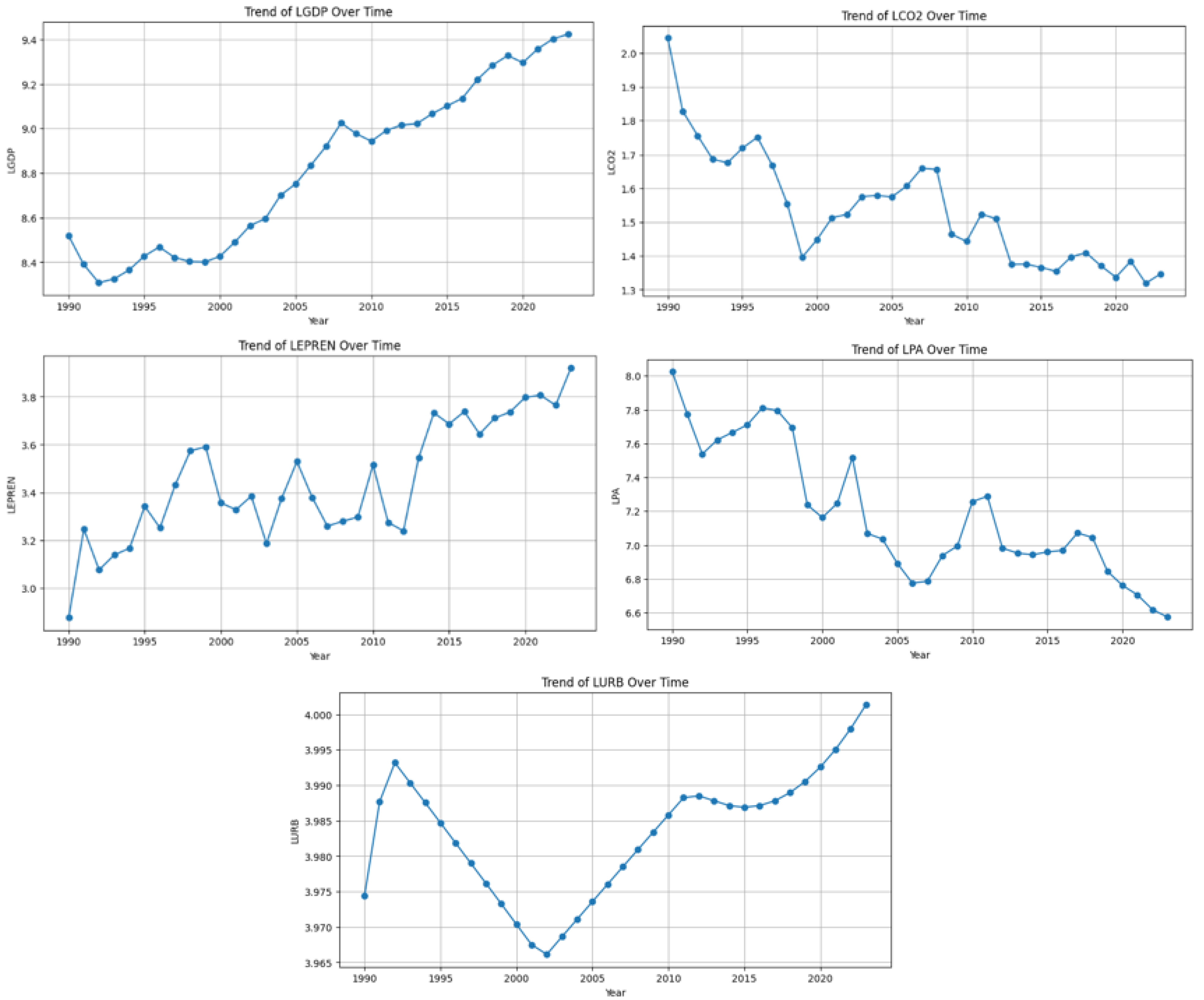
3.3. Data Collection
4. Empirical Results
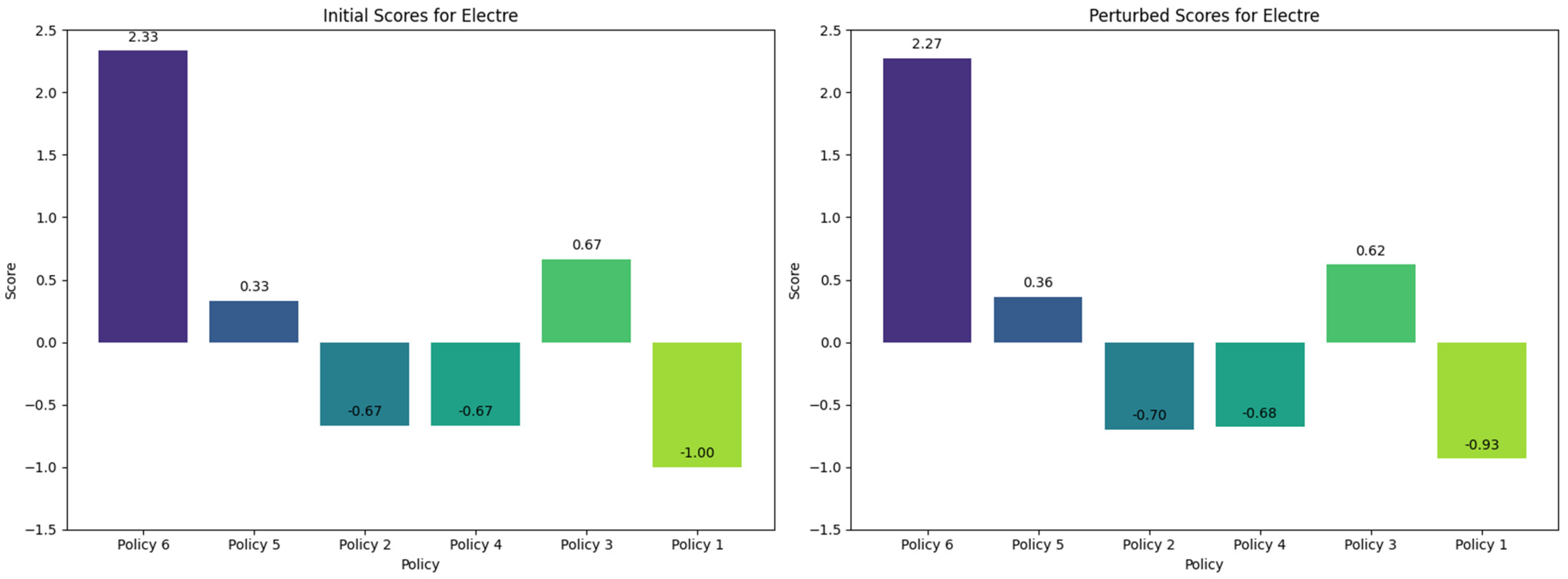
4.1. Fuzzy Electre
4.2. Fuzzy Topsis
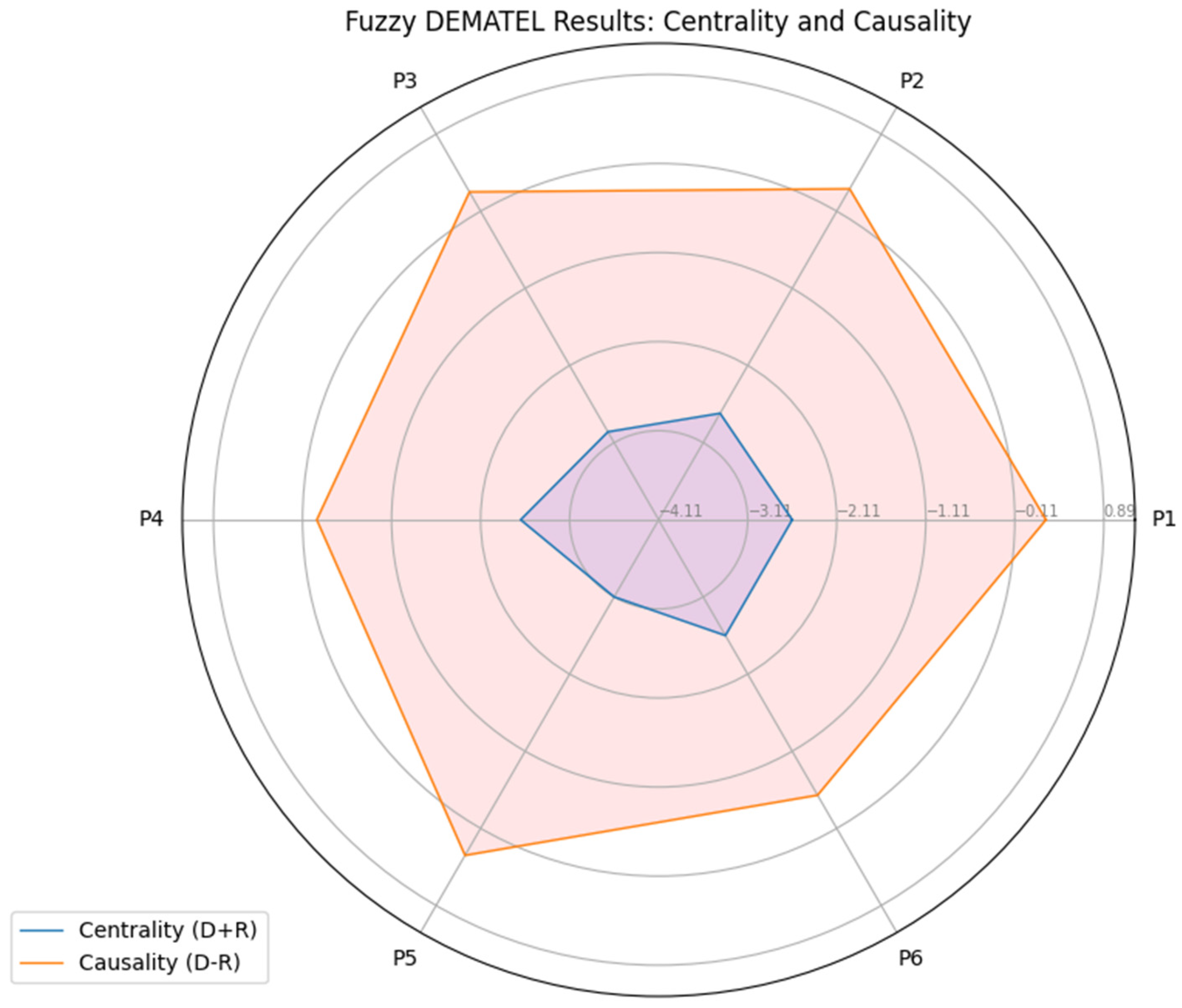
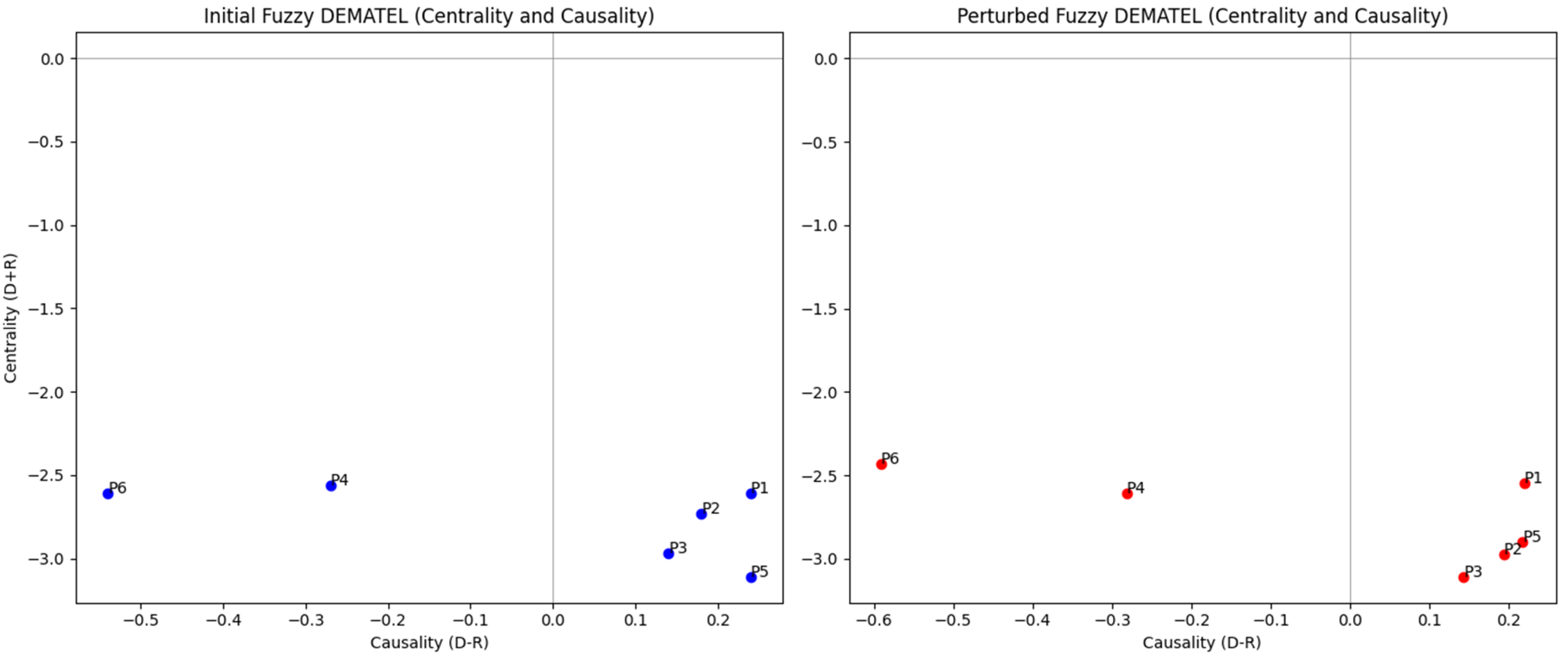
4.3. Fuzzy DEMATEL
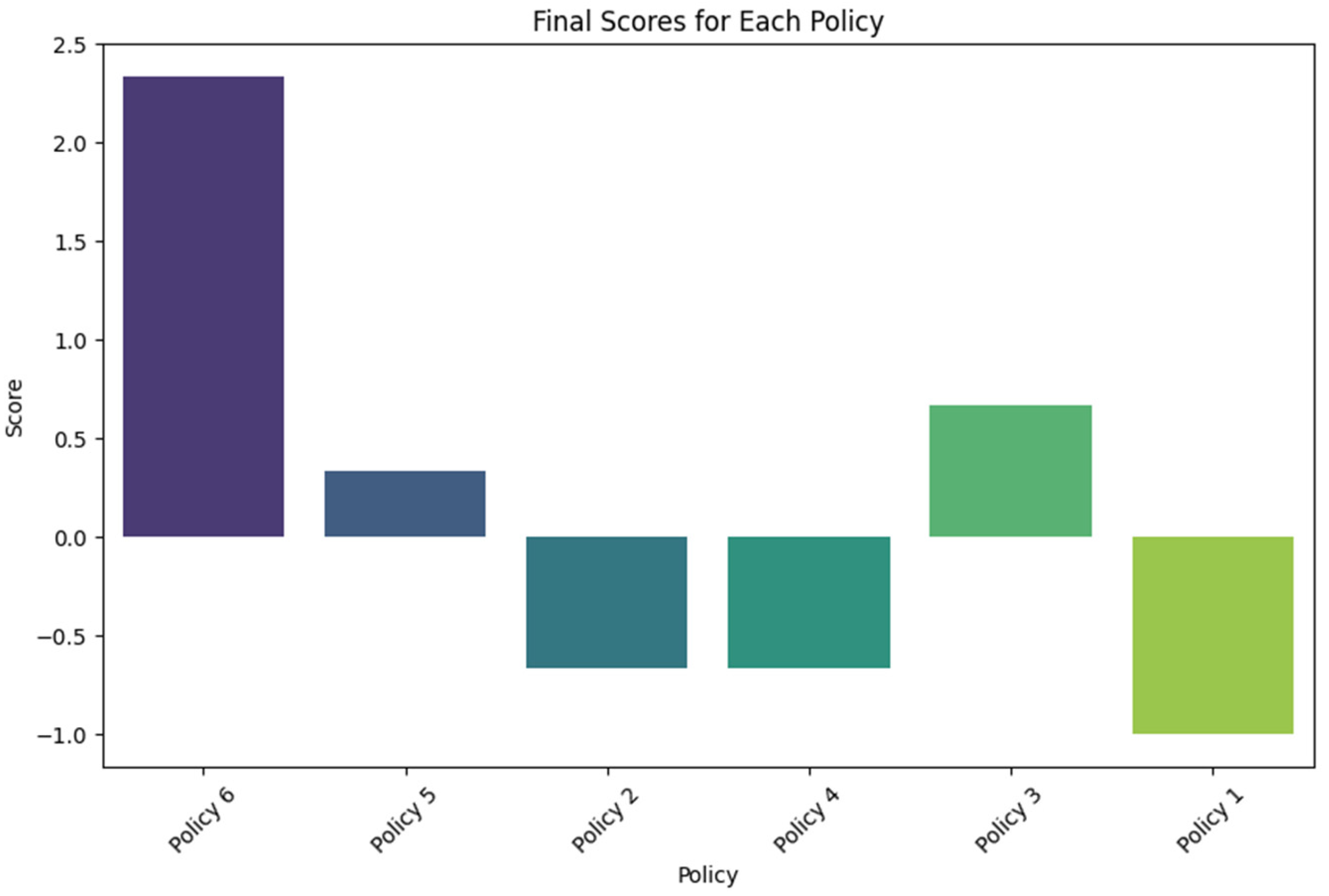
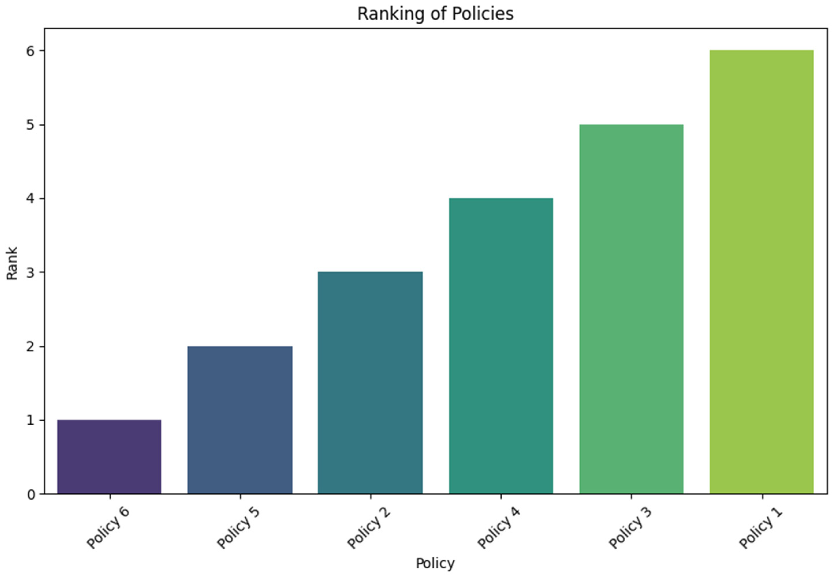
4.4. Fuzzy Vikor
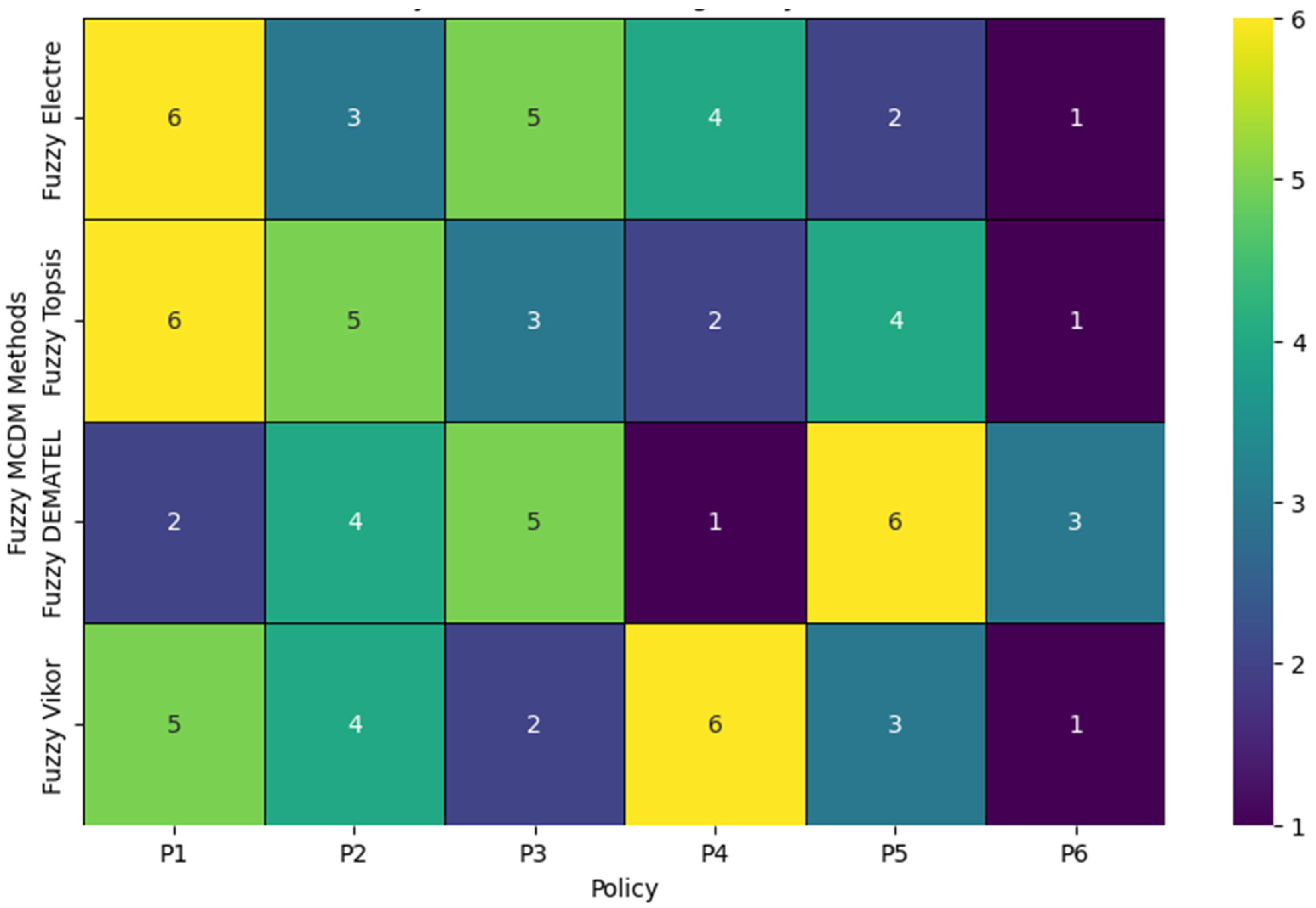
4.5. Sensitivity Analysis of Fuzzy Results
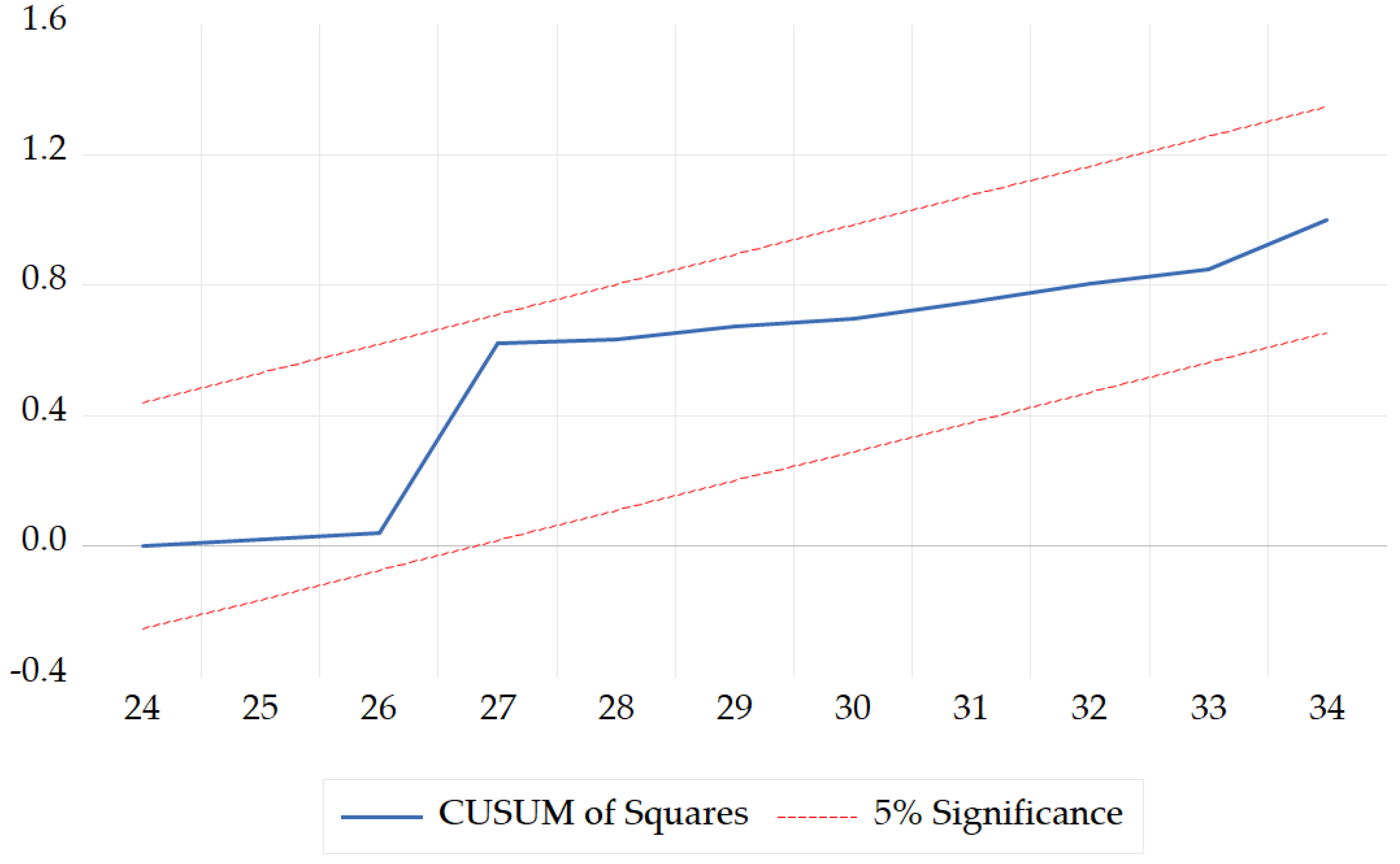
4.6. Autoregressive Distributed Lag Model
5. Conclusions and Policy Recommendations
Author Contributions
Funding
Data Availability Statement
Acknowledgments
Conflicts of Interest
Abbreviations
| Acronym | Definition |
| CE | Circular Economy |
| NSCE | National Strategy for the Circular Economy |
| MCDM | Multi-criteria decision making |
| ELECTRE | Elimination and Choice Translating Reality |
| TOPSIS | Technique for Order Preference by Similarity to Ideal Solution |
| Vikor | Multi-criteria optimization and compromise solution |
| DEMATEL | Decision-Making Trial and Evaluation Laboratory |
| FPIS | Fuzzy Positive Ideal Solution |
| FNIS | Fuzzy Negative Ideal Solution |
| CC | Closeness Coefficient |
| ARDL | Autoregressive Distributed Lag |
| ECM | Error correction model |
| ECT | Error correction term |
| ADF | Augmented Dickey–Fuller |
| VAR | Vector Autoregression |
| FPE | Final prediction error |
| AIC | Akaike information criterion |
| SC | Schwarz information criterion |
| HQ | Hannan–Quinn information criterion |
| GDP | Gross domestic product |
| PA | Patent Applications |
| EPREN | Share of energy production from renewables |
| URB | Urbanization |
References
- European Union National Strategy for the Circular Economy in Romania. Available online: https://circulareconomy.europa.eu/platform/en/strategies/national-strategy-circular-economy-romania (accessed on 8 April 2024).
- European Parliament Circular Economy: Definition, Importance and Benefits. Available online: https://www.europarl.europa.eu/topics/en/article/20151201STO05603/circular-economy-definition-importance-and-benefits (accessed on 8 April 2024).
- Yang, L.; Li, Z. Technology Advance and the Carbon Dioxide Emission in China—Empirical Research Based on the Rebound Effect. Energy Policy 2017, 101, 150–161. [Google Scholar] [CrossRef]
- Chen, Y.; Lee, C.-C. Does Technological Innovation Reduce CO2 Emissions? Cross-Country Evidence. J. Clean. Prod. 2020, 263, 121550. [Google Scholar] [CrossRef]
- Raihan, A.; Begum, R.A.; Said, M.N.M.; Pereira, J.J. Relationship between Economic Growth, Renewable Energy Use, Technological Innovation, and Carbon Emission toward Achieving Malaysia’s Paris Agreement. Env. Syst. Decis. 2022, 42, 586–607. [Google Scholar] [CrossRef]
- Sohag, K.; Begum, R.A.; Abdullah, S.M.S.; Jaafar, M. Dynamics of Energy Use, Technological Innovation, Economic Growth and Trade Openness in Malaysia. Energy 2015, 90, 1497–1507. [Google Scholar] [CrossRef]
- Liu, R.; Zhu, X.; Zhang, M.; Hu, C. Innovation Incentives and Urban Carbon Dioxide Emissions: A Quasi-Natural Experiment Based on Fast-Tracking Green Patent Applications in China. J. Clean. Prod. 2023, 382, 135444. [Google Scholar] [CrossRef]
- Wang, N.; Yu, H.; Shu, Y.; Chen, Z.; Li, T. Can Green Patents Reduce Carbon Emission Intensity?—An Empirical Analysis Based on China’s Experience. Front. Environ. Sci. 2022, 10, 1084977. [Google Scholar] [CrossRef]
- Dunyo, S.K.; Odei, S.A.; Chaiwet, W. Relationship between CO2 Emissions, Technological Innovation, and Energy Intensity: Moderating Effects of Economic and Political Uncertainty. J. Clean. Prod. 2024, 440, 140904. [Google Scholar] [CrossRef]
- Zhao, X.; Long, L.; Yin, S.; Zhou, Y. How Technological Innovation Influences Carbon Emission Efficiency for Sustainable Development? Evidence from China. Resour. Environ. Sustain. 2023, 14, 100135. [Google Scholar] [CrossRef]
- Hu, F.; Qiu, L.; Xiang, Y.; Wei, S.; Sun, H.; Hu, H.; Weng, X.; Mao, L.; Zeng, M. Spatial Network and Driving Factors of Low-Carbon Patent Applications in China from a Public Health Perspective. Front. Public. Health 2023, 11, 1121860. [Google Scholar] [CrossRef]
- Georgescu, I.; Kinnunen, J. The Role of Foreign Direct Investments, Urbanization, Productivity, and Energy Consumption in Finland’s Carbon Emissions: An ARDL Approach. Env. Sci. Pollut. Res. 2023, 30, 87685–87694. [Google Scholar] [CrossRef]
- Georgescu, I.; Kinnunen, J. Effects of FDI, GDP and Energy Use on Ecological Footprint in Finland: An ARDL Approach. World Dev. Sustain. 2024, 4, 100157. [Google Scholar] [CrossRef]
- Onofrei, M.; Vatamanu, A.F.; Cigu, E. The Relationship Between Economic Growth and CO2 Emissions in EU Countries: A Cointegration Analysis. Front. Environ. Sci. 2022, 10, 934885. [Google Scholar] [CrossRef]
- Mitić, P.; Fedajev, A.; Radulescu, M.; Rehman, A. The Relationship between CO2 Emissions, Economic Growth, Available Energy, and Employment in SEE Countries. Env. Sci. Pollut. Res. 2022, 30, 16140–16155. [Google Scholar] [CrossRef] [PubMed]
- Luqman, M.; Rayner, P.J.; Gurney, K.R. On the Impact of Urbanisation on CO2 Emissions. npj Urban. Sustain. 2023, 3, 6. [Google Scholar] [CrossRef]
- Muñoz, P.; Zwick, S.; Mirzabaev, A. The Impact of Urbanization on Austria’s Carbon Footprint. J. Clean. Prod. 2020, 263, 121326. [Google Scholar] [CrossRef]
- Chen, F.; Liu, A.; Lu, X.; Zhe, R.; Tong, J.; Akram, R. Evaluation of the Effects of Urbanization on Carbon Emissions: The Transformative Role of Government Effectiveness. Front. Energy Res. 2022, 10, 848800. [Google Scholar] [CrossRef]
- Zhang, X.; Geng, Y.; Shao, S.; Wilson, J.; Song, X.; You, W. China’s Non-Fossil Energy Development and Its 2030 CO2 Reduction Targets: The Role of Urbanization. Appl. Energy 2020, 261, 114353. [Google Scholar] [CrossRef]
- Szetela, B.; Majewska, A.; Jamroz, P.; Djalilov, B.; Salahodjaev, R. Renewable Energy and CO2 Emissions in Top Natural Resource Rents Depending Countries: The Role of Governance. Front. Energy Res. 2022, 10, 872941. [Google Scholar] [CrossRef]
- Bilan, Y.; Streimikiene, D.; Vasylieva, T.; Lyulyov, O.; Pimonenko, T.; Pavlyk, A. Linking between Renewable Energy, CO2 Emissions, and Economic Growth: Challenges for Candidates and Potential Candidates for the EU Membership. Sustainability 2019, 11, 1528. [Google Scholar] [CrossRef]
- Feng, H. The Impact of Renewable Energy on Carbon Neutrality for the Sustainable Environment: Role of Green Finance and Technology Innovations. Front. Environ. Sci. 2022, 10, 924857. [Google Scholar] [CrossRef]
- Petruška, I.; Litavcová, E.; Chovancová, J. Impact of Renewable Energy Sources and Nuclear Energy on CO2 Emissions Reductions—The Case of the EU Countries. Energies 2022, 15, 9563. [Google Scholar] [CrossRef]
- Petković, B.; Agdas, A.S.; Zandi, Y.; Nikolić, I.; Denić, N.; Radenkovic, S.D.; Almojil, S.F.; Roco-Videla, A.; Kojić, N.; Zlatković, D.; et al. Neuro Fuzzy Evaluation of Circular Economy Based on Waste Generation, Recycling, Renewable Energy, Biomass and Soil Pollution. Rhizosphere 2021, 19, 100418. [Google Scholar] [CrossRef]
- Gou, X.; Xu, X.; Xu, Z.; Skare, M. Circular Economy and Fuzzy Set Theory: A Bibliometric and Systematic Review Based on Industry 4.0 Technologies Perspective. Technol. Econ. Dev. Econ. 2024, 30, 489–526. [Google Scholar] [CrossRef]
- Bai, C.; Zhu, Q.; Sarkis, J. Circular Economy and Circularity Supplier Selection: A Fuzzy Group Decision Approach. Int. J. Prod. Res. 2024, 62, 2307–2330. [Google Scholar] [CrossRef]
- Abdelmeguid, A.; Afy-Shararah, M.; Salonitis, K. Mapping of the Circular Economy Implementation Challenges in the Fashion Industry: A Fuzzy-TISM Analysis. Circ. Econ. Sust. 2024, 4, 585–617. [Google Scholar] [CrossRef]
- Husain, Z.; Maqbool, A.; Haleem, A.; Pathak, R.D.; Samson, D. Analyzing the Business Models for Circular Economy Implementation: A Fuzzy TOPSIS Approach. Oper. Manag. Res. 2021, 14, 256–271. [Google Scholar] [CrossRef]
- Damgaci, E.; Boran, K.; Boran, F.E. Evaluation of Turkey’s Renewable Energy Using Intuitionistic Fuzzy Topsis Method. J. Polytech. -Politek. Derg. 2017, 20, 629–637. [Google Scholar]
- Soft Computing Applications for Renewable Energy and Energy Efficiency; Cascales, M.D.S.G.; Lozano, J.M.S.; Arredondo, A.D.M.; Corona, C.C. (Eds.) Advances in Environmental Engineering and Green Technologies; IGI Global: Hershey, PA, USA, 2015; ISBN 978-1-4666-6631-3. [Google Scholar]
- Khan, S.; Haleem, A. Strategies to Implement Circular Economy Practices: A Fuzzy DEMATEL Approach. J. Ind. Intg. Mgmt. 2020, 05, 253–269. [Google Scholar] [CrossRef]
- Boran, F.E.; Boran, K.; Menlik, T. The Evaluation of Renewable Energy Technologies for Electricity Generation in Turkey Using Intuitionistic Fuzzy TOPSIS. Energy Sources Part B Econ. Plan. Policy 2012, 7, 81–90. [Google Scholar] [CrossRef]
- Kaya, T.; Kahraman, C. Multicriteria Renewable Energy Planning Using an Integrated Fuzzy VIKOR & AHP Methodology: The Case of Istanbul. Energy 2010, 35, 2517–2527. [Google Scholar] [CrossRef]
- Li, T.; Wang, H.; Lin, Y. Selection of Renewable Energy Development Path for Sustainable Development Using a Fuzzy MCDM Based on Cumulative Prospect Theory: The Case of Malaysia. Sci. Rep. 2024, 14, 15082. [Google Scholar] [CrossRef] [PubMed]
- Riaz, M.; Habib, A.; Saqlain, M.; Yang, M.-S. Cubic Bipolar Fuzzy-VIKOR Method Using New Distance and Entropy Measures and Einstein Averaging Aggregation Operators with Application to Renewable Energy. Int. J. Fuzzy Syst. 2023, 25, 510–543. [Google Scholar] [CrossRef]
- Simmhan, Y.; Ingen, C.V.; Szalay, A.; Barga, R.; Heasley, J. Building Reliable Data Pipelines for Managing Community Data Using Scientific Workflows. In Proceedings of the 2009 Fifth IEEE International Conference on e-Science, Oxford, UK, 9–11 December 2009; IEEE: Oxford, UK, 2009; pp. 321–328. [Google Scholar]
- Govindan, K.; Nasr, A.K.; Karimi, F.; Mina, H. Circular Economy Adoption Barriers: An Extended Fuzzy Best–Worst Method Using Fuzzy DEMATEL and Supermatrix Structure. Bus. Strat. Env. 2022, 31, 1566–1586. [Google Scholar] [CrossRef]
- Ayçin, E.; Kayapinar Kaya, S. Towards the Circular Economy: Analysis of Barriers to Implementation of Turkey’s Zero Waste Management Using the Fuzzy DEMATEL Method. Waste Manag. Res. 2021, 39, 1078–1089. [Google Scholar] [CrossRef]
- Turgut, Z.K.; Tolga, A.Ç. Fuzzy MCDM Methods in Sustainable and Renewable Energy Alternative Selection: Fuzzy VIKOR and Fuzzy TODIM. In Energy Management—Collective and Computational Intelligence with Theory and Applications; Kahraman, C., Kayakutlu, G., Eds.; Studies in Systems, Decision and Control; Springer International Publishing: Cham, Switzerland, 2018; Volume 149, pp. 277–314. ISBN 978-3-319-75689-9. [Google Scholar]
- Rejeb, A.; Rejeb, K.; Keogh, J.G.; Zailani, S. Barriers to Blockchain Adoption in the Circular Economy: A Fuzzy Delphi and Best-Worst Approach. Sustainability 2022, 14, 3611. [Google Scholar] [CrossRef]
- Khan, F.; Ali, Y. A Facilitating Framework for a Developing Country to Adopt Smart Waste Management in the Context of Circular Economy. Env. Sci. Pollut. Res. 2022, 29, 26336–26351. [Google Scholar] [CrossRef]
- Poonia, V.; Kulshrestha, R.; Sangwan, K.S.; Sharma, S. A Multi-Objective Fuzzy Mathematical Model for Circular Economy with Leasing as a Strategy. MEQ 2024. [Google Scholar] [CrossRef]
- Zadeh, L.A. Fuzzy Sets. Inf. Control 1965, 8, 338–353. [Google Scholar] [CrossRef]
- Bellman, R.E.; Zadeh, L.A. Decision-Making in a Fuzzy Environment. Manag. Sci. 1970, 17, 141–164. [Google Scholar] [CrossRef]
- Wang, T.-C.; Chang, T.-H. Application of TOPSIS in Evaluating Initial Training Aircraft under a Fuzzy Environment. Expert. Syst. Appl. 2007, 33, 870–880. [Google Scholar] [CrossRef]
- Awasthi, A.; Chauhan, S.S.; Goyal, S.K. A Fuzzy Multicriteria Approach for Evaluating Environmental Performance of Suppliers. Int. J. Prod. Econ. 2010, 126, 370–378. [Google Scholar] [CrossRef]
- Wu, W.-W.; Lee, Y.-T. Developing Global Managers’ Competencies Using the Fuzzy DEMATEL Method. Expert. Syst. Appl. 2007, 32, 499–507. [Google Scholar] [CrossRef]
- Opricovic, S.; Tzeng, G.-H. Compromise Solution by MCDM Methods: A Comparative Analysis of VIKOR and TOPSIS. Eur. J. Oper. Res. 2004, 156, 445–455. [Google Scholar] [CrossRef]
- Mardani, A.; Zavadskas, E.; Govindan, K.; Amat Senin, A.; Jusoh, A. VIKOR Technique: A Systematic Review of the State of the Art Literature on Methodologies and Applications. Sustainability 2016, 8, 37. [Google Scholar] [CrossRef]
- Roy, B.; Bertier, P. La Méthode Electre II—Une Methode Au Media-Planning. Oper. Res. 1973, 291–302. [Google Scholar]
- Akram, M.; Zahid, K.; Kahraman, C. A New ELECTRE-Based Decision-Making Framework with Spherical Fuzzy Information for the Implementation of Autonomous Vehicles Project in Istanbul. Knowl. Based Syst. 2024, 283, 111207. [Google Scholar] [CrossRef]
- Daneshvar Rouyendegh, B.; Erol, S. Selecting the Best Project Using the Fuzzy ELECTRE Method. Math. Probl. Eng. 2012, 2012, 790142. [Google Scholar] [CrossRef]
- Dubois, D.; Prade, H. Fuzzy Sets and Systems: Theory and Applications, 1st ed.; Elsevier Science: New York, NY, USA, 1980; Volume 144, ISBN 978-0-12-399465-3. [Google Scholar]
- Komsiyah, S.; Wongso, R.; Pratiwi, S.W. Applications of the Fuzzy ELECTRE Method for Decision Support Systems of Cement Vendor Selection. Procedia Comput. Sci. 2019, 157, 479–488. [Google Scholar] [CrossRef]
- Fuzzy Multi-Criteria Decision Making; Kahraman, C. (Ed.) Springer Optimization and Its Applications; Springer: Boston, MA, USA, 2008; Volume 16, ISBN 978-0-387-76812-0. [Google Scholar]
- Montanari, R.; Micale, R.; Bottani, E.; Volpi, A.; La Scalia, G. Evaluation of Routing Policies Using an Interval-Valued TOPSIS Approach for the Allocation Rules. Comput. Ind. Eng. 2021, 156, 107256. [Google Scholar] [CrossRef]
- Wanke, P.; Pestana Barros, C.; Chen, Z. An Analysis of Asian Airlines Efficiency with Two-Stage TOPSIS and MCMC Generalized Linear Mixed Models. Int. J. Prod. Econ. 2015, 169, 110–126. [Google Scholar] [CrossRef]
- Arantes, R.F.M.; Zanon, L.G.; Calache, L.D.D.R.; Bertassini, A.C.; Carpinetti, L.C.R. A Fuzzy Multicriteria Group Decision Approach for Circular Business Models Prioritization. Production 2022, 32, e20220019. [Google Scholar] [CrossRef]
- Haleem, A.; Khan, S.; Luthra, S.; Varshney, H.; Alam, M.; Khan, M.I. Supplier Evaluation in the Context of Circular Economy: A Forward Step for Resilient Business and Environment Concern. Bus. Strat. Env. 2021, 30, 2119–2146. [Google Scholar] [CrossRef]
- Chen, C.-T. Extensions of the TOPSIS for Group Decision-Making under Fuzzy Environment. Fuzzy Sets Syst. 2000, 114, 1–9. [Google Scholar] [CrossRef]
- Awasthi, A.; Chauhan, S.S.; Goyal, S.K. A Multi-Criteria Decision Making Approach for Location Planning for Urban Distribution Centers under Uncertainty. Math. Comput. Model. 2011, 53, 98–109. [Google Scholar] [CrossRef]
- Nădăban, S.; Dzitac, S.; Dzitac, I. Fuzzy TOPSIS: A General View. Procedia Comput. Sci. 2016, 91, 823–831. [Google Scholar] [CrossRef]
- Opricovic, S.; Tzeng, G.-H. Extended VIKOR Method in Comparison with Outranking Methods. Eur. J. Oper. Res. 2007, 178, 514–529. [Google Scholar] [CrossRef]
- Yazdani, M.; Graeml, F.R. VIKOR and its Applications: A State-of-the-Art Survey. Int. J. Strateg. Decis. Sci. 2014, 5, 56–83. [Google Scholar] [CrossRef]
- Kizielewicz, B.; Bączkiewicz, A. Comparison of Fuzzy TOPSIS, Fuzzy VIKOR, Fuzzy WASPAS and Fuzzy MMOORA Methods in the Housing Selection Problem. Procedia Comput. Sci. 2021, 192, 4578–4591. [Google Scholar] [CrossRef]
- Chang, B.; Chang, C.-W.; Wu, C.-H. Fuzzy DEMATEL Method for Developing Supplier Selection Criteria. Expert. Syst. Appl. 2011, 38, 1850–1858. [Google Scholar] [CrossRef]
- Lütkepohl, H.; Xu, F. The Role of the Log Transformation in Forecasting Economic Variables. Empir. Econ. 2012, 42, 619–638. [Google Scholar] [CrossRef]
- Bayer, C.; Hanck, C. Combining Non-cointegration Tests. J. Time Ser. Anal. 2013, 34, 83–95. [Google Scholar] [CrossRef]
- Engle, R.F.; Granger, C.W.J. Co-Integration and Error Correction: Representation, Estimation, and Testing. Econometrica 1987, 55, 251. [Google Scholar] [CrossRef]
- Johansen, S. Statistical Analysis of Cointegration Vectors. J. Econ. Dyn. Control 1988, 12, 231–254. [Google Scholar] [CrossRef]
- Peter Boswijk, H. Testing for an Unstable Root in Conditional and Structural Error Correction Models. J. Econom. 1994, 63, 37–60. [Google Scholar] [CrossRef]
- Banerjee, A.; Dolado, J.; Mestre, R. Error-correction Mechanism Tests for Cointegration in a Single-equation Framework. J. Time Ser. Anal. 1998, 19, 267–283. [Google Scholar] [CrossRef]
- Pesaran, M.H.; Shin, Y.; Smith, R.J. Bounds Testing Approaches to the Analysis of Level Relationships. J. Appl. Econom. 2001, 16, 289–326. [Google Scholar] [CrossRef]
- Our World in Data Per Capital CO2 Emissions (Tonnes). Available online: https://ourworldindata.org/co2-and-greenhouse-gas-emissions (accessed on 7 September 2024).
- World Bank Patent Applications, Residents. Available online: https://data.worldbank.org/indicator/IP.PAT.RESD (accessed on 7 September 2024).
- World Bank Patent Applications, Nonresidents. Available online: https://data.worldbank.org/indicator/IP.PAT.NRES (accessed on 7 September 2024).
- World Bank GDP per Capita (Constant 2015 US$). Available online: https://data.worldbank.org/indicator/NY.GDP.PCAP.KD (accessed on 7 September 2024).
- Our World in Data Share of Electricity Production from Renewables 2023.
- World Bank Urban Population (% of Total Population). Available online: https://data.worldbank.org/indicator/SP.URB.TOTL.IN.ZS (accessed on 7 September 2024).
- Giovanis, E. Relationship between Recycling Rate and Air Pollution: Waste Management in the State of Massachusetts. Waste Manag. 2015, 40, 192–203. [Google Scholar] [CrossRef]
- Sidique, S.F.; Joshi, S.V.; Lupi, F. Factors Influencing the Rate of Recycling: An Analysis of Minnesota Counties. Resour. Conserv. Recycl. 2010, 54, 242–249. [Google Scholar] [CrossRef]
- Nastase, C.; Chașovschi, C.E.; State, M.; Scutariu, A.-L. Municipal Waste Management in Romania in The context of the EU. A Stakeholders’ Perspective. Technol. Econ. Dev. Econ. 2019, 25, 850–876. [Google Scholar] [CrossRef]
- Delcea, C.; Crăciun, L.; Ioanăș, C.; Ferruzzi, G.; Cotfas, L.-A. Determinants of Individuals’ E-Waste Recycling Decision: A Case Study from Romania. Sustainability 2020, 12, 2753. [Google Scholar] [CrossRef]
- Aceleanu, M.I.; Șerban, A.C.; Pociovălișteanu, D.M.; Dimian, G.C. Renewable Energy: A Way for a Sustainable Development in Romania. Energy Sources Part B Econ. Plan. Policy 2017, 12, 958–963. [Google Scholar] [CrossRef]
- Vanegas Cantarero, M.M. Of Renewable Energy, Energy Democracy, and Sustainable Development: A Roadmap to Accelerate the Energy Transition in Developing Countries. Energy Res. Soc. Sci. 2020, 70, 101716. [Google Scholar] [CrossRef]
- Jefferson, M. Accelerating the Transition to Sustainable Energy Systems. Energy Policy 2008, 36, 4116–4125. [Google Scholar] [CrossRef]
- Prăvălie, R.; Sîrodoev, I.; Ruiz-Arias, J.; Dumitraşcu, M. Using Renewable (Solar) Energy as a Sustainable Management Pathway of Lands Highly Sensitive to Degradation in Romania. A Countrywide Analysis Based on Exploring the Geographical and Technical Solar Potentials. Renew. Energy 2022, 193, 976–990. [Google Scholar] [CrossRef]
- Dobre-Baron, O.; Nițescu, A.; Niță, D.; Mitran, C. Romania’s Perspectives on the Transition to the Circular Economy in an EU Context. Sustainability 2022, 14, 5324. [Google Scholar] [CrossRef]
- Topliceanu, L.; Puiu, P.G.; Drob, C.; Topliceanu, V.V. Analysis Regarding the Implementation of the Circular Economy in Romania. Sustainability 2022, 15, 333. [Google Scholar] [CrossRef]
- Botezat, E.A.; Dodescu, A.O.; Văduva, S.; Fotea, S.L. An Exploration of Circular Economy Practices and Performance Among Romanian Producers. Sustainability 2018, 10, 3191. [Google Scholar] [CrossRef]
- Aceleanu, M.I.; Serban, A.C.; Suciu, M.-C.; Bitoiu, T.I. The Management of Municipal Waste through Circular Economy in the Context of Smart Cities Development. IEEE Access 2019, 7, 133602–133614. [Google Scholar] [CrossRef]
- Platon, V.; Pavelescu, F.M.; Antonescu, D.; Frone, S.; Constantinescu, A.; Popa, F. Innovation and Recycling—Drivers of Circular Economy in EU. Front. Environ. Sci. 2022, 10, 902651. [Google Scholar] [CrossRef]
- Lakatos, E.; Cioca, L.-I.; Dan, V.; Ciomos, A.; Crisan, O.; Barsan, G. Studies and Investigation about the Attitude towards Sustainable Production, Consumption and Waste Generation in Line with Circular Economy in Romania. Sustainability 2018, 10, 865. [Google Scholar] [CrossRef]
- Dinu, M.; Pătărlăgeanu, S.R.; Petrariu, R.; Constantin, M.; Potcovaru, A.-M. Empowering Sustainable Consumer Behavior in the EU by Consolidating the Roles of Waste Recycling and Energy Productivity. Sustainability 2020, 12, 9794. [Google Scholar] [CrossRef]
- Liobikienė, G.; Dagiliūtė, R. The Relationship between Economic and Carbon Footprint Changes in EU: The Achievements of the EU Sustainable Consumption and Production Policy Implementation. Environ. Sci. Policy 2016, 61, 204–211. [Google Scholar] [CrossRef]
- Firoiu, D.; Ionescu, G.H.; Băndoi, A.; Florea, N.M.; Jianu, E. Achieving Sustainable Development Goals (SDG): Implementation of the 2030 Agenda in Romania. Sustainability 2019, 11, 2156. [Google Scholar] [CrossRef]
- Oroian, C.; Safirescu, C.; Harun, R.; Chiciudean, G.; Arion, F.; Muresan, I.; Bordeanu, B. Consumers’ Attitudes towards Organic Products and Sustainable Development: A Case Study of Romania. Sustainability 2017, 9, 1559. [Google Scholar] [CrossRef]
- OECD Resource Efficiency and Circular Economy. Available online: https://www.oecd.org/en/topics/policy-issues/resource-efficiency-and-circular-economy.html (accessed on 8 April 2024).
- Mocanu, A.A.; Brătucu, G.; Ciobanu, E.; Chițu, I.B.; Szakal, A.C. Can the Circular Economy Unlock Sustainable Business Growth? Insights from Qualitative Research with Specialists in Romania. Sustainability 2024, 16, 2031. [Google Scholar] [CrossRef]
- Andrei, J.; Mieila, M.; Popescu, G.; Nica, E.; Cristina, M. The Impact and Determinants of Environmental Taxation on Economic Growth Communities in Romania. Energies 2016, 9, 902. [Google Scholar] [CrossRef]
- Busu, M. Adopting Circular Economy at the European Union Level and Its Impact on Economic Growth. Soc. Sci. 2019, 8, 159. [Google Scholar] [CrossRef]
- Mihaela Cristina, D.; Maria-Floriana, P.; Jean Vasile, A.; Mihai, M. Developments of the Circular Economy in Romania under the New Sustainability Paradigm. Econ. Comput. Econ. Cybern. Stud. Res. 2018, 52, 125–138. [Google Scholar] [CrossRef]
- Trica, C.L.; Banacu, C.S.; Busu, M. Environmental Factors and Sustainability of the Circular Economy Model at the European Union Level. Sustainability 2019, 11, 1114. [Google Scholar] [CrossRef]
- Nica, I.; Chiriță, N.; Delcea, C. Towards a Sustainable Future: Economic Cybernetics in Analyzing Romania’s Circular Economy. Sustainability 2023, 15, 14433. [Google Scholar] [CrossRef]
- Nica, I.; Ciocan, M.-L. Mapping Circular Pathways: A Bibliometric Exploration and Multilinear Regression Model of Romania’s Circular Economy. Theor. Appl. Econ. 2023, 30, 17–34. [Google Scholar]
- Chiriță, N.; Georgescu, I. Cybernetics Analysis of the Circular Economy from Romania. In Proceedings of 22nd International Conference on Informatics in Economy (IE 2023); Ciurea, C., Pocatilu, P., Filip, F.G., Eds.; Smart Innovation, Systems and Technologies; Springer Nature: Singapore, 2024; Volume 367, pp. 319–330. ISBN 978-981-9969-59-3. [Google Scholar]
- Cioca, L.-I.; Ivascu, L.; Rada, E.; Torretta, V.; Ionescu, G. Sustainable Development and Technological Impact on CO2 Reducing Conditions in Romania. Sustainability 2015, 7, 1637–1650. [Google Scholar] [CrossRef]
- Hatmanu, M.; Cautisanu, C.; Iacobuta, A.O. On the Relationships between CO2 Emissions and Their Determinants in Romania and Bulgaria. An ARDL Approach. Appl. Econ. 2022, 54, 2582–2595. [Google Scholar] [CrossRef]
- Busu, M. Measuring the Renewable Energy Efficiency at the European Union Level and Its Impact on CO2 Emissions. Processes 2019, 7, 923. [Google Scholar] [CrossRef]
- Dickey, D.A.; Fuller, W.A. Distribution of the Estimators for Autoregressive Time Series with a Unit Root. J. Am. Stat. Assoc. 1979, 74, 427–431. [Google Scholar] [CrossRef]


| Authors, Year, References | Scope | Technique | Criteria |
|---|---|---|---|
| Husain et al., 2021, [28] | Classification of business models for the successful adoption of the CE | Fuzzy Topsis | Partnership; Activities; Resources; Value proposition; Customer Relationships; Distribution Channels; Client Segments; Cost structure; Revenue flows; |
| Damgaci et al., 2017, [29] | Evaluation of Turkey’s Renewable Energy | Intuitionistic Fuzzy Topsis | Technical; Economical; Environmental; Social; |
| Öztayşi and Kahraman, 2015, [30] | Evaluation of Renewable Energies Alternatives | Interval Type-2 Fuzzy AHP; Hesitant Fuzzy Topsis | Renewable energy factors; uncertainty; linguistic preference; |
| Khan and Haleem, 2020, [31] | Identifying and evaluating key strategies for adopting circular economy practices | Fuzzy DEMATEL | 11 strategies for adopting the CE, including involving management, creating a vision and goals; |
| Boran et al., 2012, [32] | Assessment of renewable energy technologies for electricity generation in Turkey | Intuitionistic Fuzzy Topsis | Renewable Energy Technologies: Photovoltaic, Hydro, Wind, Geothermal |
| Kaya and Kahraman, 2010, [33] | Determining the best renewable energy alternative and optimal location for production in Istanbul | Integrated Fuzzy VIKOR-AHP | Criteria for the selection of renewable energy and location: technical, economic, geographical, social |
| Li et al., 2024, [34] | Identifying the most suitable renewable energy source for Malaysia’s sustainable development | Fuzzy Multi-Criteria Decision Making (MCDM) based on cumulative prospect theory | Technology, economy, society, environment; Efficiency, payback period, job creation, CO2 emissions |
| Riaz et al., 2023, [35] | Application of cubic bipolar fuzzy sets for the selection of the best renewable energy source | Cubic Bipolar Fuzzy Set (CBFS), CBF-VIKOR, Einstein averaging aggregation operators | Selection of renewable energy sources |
| Simmhan et al., 2009, [36] | Evaluation of the development of the circular economy in the coal mining industry | Membership transformation algorithm, fuzzy evaluation | Developing the circular economy in coal mining, dynamic assessment |
| Govindan et al., 2022, [37] | Prioritizing barriers to circular economy adoption in the cable and wire industry | Fuzzy Best-Worst Method (BWM), Fuzzy DEMATEL, Super matrix | Barriers to circular economy adoption: installation costs, financial limitations, lack of public awareness, etc. |
| Ayçin and Kayapinar Kaya, 2021, [38] | Identification of barriers to the implementation of the zero-waste strategy in Turkey in the context of the circular economy | Fuzzy DEMATEL | 12 key barriers to zero waste implementation: uncertainty of goals, lack of financial aid, etc. |
| Turgut and Tolga, 2018, [39] | Evaluation and selection of the best sustainable and/or renewable energy alternative | Fuzzy VIKOR, Fuzzy TODIM, Sensitivity Analysis | Renewable Energy: Solar, Wind, Hydroelectric, Storage Gas (LFG) |
| Rejeb et al., 2022, [40] | Identifying and prioritizing barriers in the adoption of blockchain technology in the circular economy | Fuzzy Delphi, Best-Worst Method (BWM) | 16 barriers to blockchain adoption in the CE: lack of knowledge, reluctance to change, technological immaturity |
| Khan and Ali, 2022, [41] | Creating a framework for the adoption of smart waste management in the context of the circular economy for Pakistan | Fuzzy SWARA, Fuzzy VIKOR | 16 critical enablers for the adoption of smart waste management, including regulations, industry responsibility, digitalization (ICT and IoT) |
| Poonia et al., 2024, [42] | Development of a multi-objective mathematical model for the circular economy, integrating leasing and other strategies | Multi-objective Fuzzy Mixed Integer Linear Programming | Economic, environmental and social objectives; the concept of leasing, reuse, refurbishment, primary and secondary recycling |
| Variable | Acronym | Measurement Unit | Source |
|---|---|---|---|
| emissions per capita | CO2 | Tons | Our World in Data [74] |
| Patent applications | PA | Number | World Bank [75,76] |
| Gross domestic product | GDP | Constant 2015 $USD | World Bank [77] |
| Share of energy production from renewables | EPREN | % | Our World in Data [78] |
| Urbanization | URB | % | World Bank [79] |
| Criteria | Policy |
|---|---|
| Waste recycling rate | Waste management policy (P1): Studies show that effective waste management policies can significantly increase recycling rates. Implementation of these policies leads to more efficient waste management and reduced environmental impacts [80,81,82,83]. |
| Installed capacity of renewable energy | Energy efficiency policy (P2): There is a direct link between energy efficiency policies and the increase in installed renewable energy capacity. This is due to investments in more efficient technologies and the transition to more sustainable energy sources [84,85,86,87]. |
| Investments in CE technologies | Innovation and development (P3): Investments in innovation and development are essential to advance circular technologies. They enable the development of more efficient processes and products, thereby reducing the impact on resources [88,89,90,91,92]. |
| Materials consumption per capita | Sustainable production and consumption (P4): By implementing policies that promote responsible consumption, per capita material consumption can be significantly reduced [93,94,95,96,97]. This includes consumer education and regulations that encourage resource efficiency [98,99]. |
| GDP from circular activities | GDP growth through the CE (P5): studies show that economies that adopt circular models can see an increase in GDP due to innovation and the creation of new markets and jobs [100,101,102,103,104,105,106]. |
| emissions per capita of GDP | Reducing emissions (P6): Policies to reduce emissions are fundamental to improving the carbon efficiency of the economy [107,108,109]. This is achieved by promoting green energy and optimizing industrial processes. |
| Fuzzy Linguistic Terms | Triangular Fuzzy Number Interval |
|---|---|
| Very High Importance (VHI) | [0.8, 0.9, 1.0] |
| High Importance (HI) | [0.7, 0.8, 0.9] |
| Moderately High Importance (MHI) | [0.6, 0.7, 0.8] |
| Medium Importance (MI) | [0.5, 0.6, 0.7] |
| Moderately Low Importance (MLI) | [0.4, 0.5, 0.6] |
| Low Importance (LI) | [0.3, 0.4, 0.5] |
| Very Low Importance (VLI) | [0.2, 0.3, 0.4] |
| Policy | Waste Recycling Rate | Installed Capacity of Renewable Energy | Investments in Circular Economy Technologies | Materials Consumption per Capita | GDP from Circular Activities | Emissions per Capita of GDP |
|---|---|---|---|---|---|---|
| Waste management (P1) | [0.7, 0.8, 0.9] (HI) | [0.3, 0.4, 0.5] (LI) | [0.4, 0.5, 0.6] (MLI) | [0.2, 0.3, 0.4] (VLI) | [0.6, 0.7, 0.8] (MHI) | [0.4, 0.5, 0.6] (MLI) |
| Energy efficiency (P2) | [0.5, 0.6, 0.7] (MI) | [0.7, 0.8, 0.9] (HI) | [0.3, 0.4, 0.5] (LI) | [0.3, 0.4, 0.5] (LI) | [0.5, 0.6, 0.7] (MI) | [0.5, 0.6, 0.7] (MI) |
| Innovation and development (P3) | [0.6, 0.7, 0.8] (MHI) | [0.5, 0.6, 0.7] (MI) | [0.8, 0.9, 1.00] (VHI) | [0.4, 0.5, 0.6] (MLI) | [0.6, 0.7, 0.8] (MHI) | [0.3, 0.4, 0.5] (LI) |
| Sustainable production and consumption (P4) | [0.3, 0.4, 0.5] (LI) | [0.4, 0.5, 0.6] (MLI) | [0.5, 0.6, 0.7] (MI) | [0.7, 0.8, 0.9] (HI) | [0.4, 0.5, 0.6] (MLI) | [0.6, 0.7, 0.8] (MHI) |
| GDP growth through CE (P5) | [0.4, 0.5, 0.6] (MLI) | [0.6, 0.7, 0.8] (MHI) | [0.7, 0.8, 0.9] (HI) | [0.5, 0.6, 0.7] (MI) | [0.8, 0.9, 1.00] (VHI) | [0.2, 0.3, 0.4] (VLI) |
| Reducing CO2 emissions (P6) | [0.5, 0.6, 0.7] (MI) | [0.8, 0.9, 1.00] (VHI) | [0.6, 0.7, 0.8] (MHI) | [0.6, 0.7, 0.8] (MHI) | [0.7, 0.8, 0.9] (HI) | [0.4, 0.5, 0.6] (MLI) |
| Criteria | Fuzzy Weights | Linguistic Term |
|---|---|---|
| Waste recycling rate | [0.1, 0.2, 0.3] | Moderate importance |
| Installed capacity of renewable energy | [0.2, 0.3, 0.4] | Higher importance |
| Investments in CE technologies | [0.15, 0.25, 0.35] | Medium importance |
| Materials consumption per capita | [0.1, 0.2, 0.3] | Moderate importance |
| GDP from circular activities | [0.25, 0.35, 0.45] | Higher importance |
| emissions per capita of GDP | [0.2, 0.3, 0.4] | Higher importance |
| P1 | P2 | P3 | P4 | P5 | P6 | |
|---|---|---|---|---|---|---|
| P1 | 0.00 | 0.50 | 0.50 | 0.33 | 0.33 | 0.33 |
| P2 | 0.50 | 0.00 | 0.33 | 0.50 | 0.50 | 0.33 |
| P3 | 0.67 | 0.67 | 0.00 | 0.67 | 0.50 | 0.33 |
| P4 | 0.67 | 0.50 | 0.33 | 0.00 | 0.33 | 0.33 |
| P5 | 0.67 | 0.50 | 0.50 | 0.67 | 0.00 | 0.33 |
| P6 | 0.83 | 0.83 | 0.67 | 0.67 | 0.67 | 0.00 |
| P1 | P2 | P3 | P4 | P5 | P6 | |
|---|---|---|---|---|---|---|
| P1 | 0.00 | 0.50 | 0.50 | 0.67 | 0.67 | 0.67 |
| P2 | 0.50 | 0.00 | 0.67 | 0.50 | 0.50 | 0.67 |
| P3 | 0.33 | 0.33 | 0.00 | 0.33 | 0.50 | 0.67 |
| P4 | 0.33 | 0.50 | 0.67 | 0.00 | 0.67 | 0.67 |
| P5 | 0.33 | 0.50 | 0.50 | 0.33 | 0.00 | 0.67 |
| P6 | 0.17 | 0.17 | 0.33 | 0.33 | 0.33 | 0.00 |
| Criteria | Closeness Coefficient (CC) | Rank |
|---|---|---|
| P1 | 0.35 | 6 |
| P2 | 0.42 | 5 |
| P3 | 0.53 | 3 |
| P4 | 0.41 | 2 |
| P5 | 0.56 | 4 |
| P6 | 0.70 | 1 |
| Criteria | Centrality (D + R) | Causality (D − R) |
|---|---|---|
| P1 | −2.61 | 0.24 |
| P2 | −2.73 | 0.18 |
| P3 | −2.97 | 0.14 |
| P4 | −2.56 | −0.27 |
| P5 | −3.11 | 0.24 |
| P6 | −2.61 | −0.54 |
| Policy | S | R | Q | Rank |
|---|---|---|---|---|
| P1 | 1.02 | 0.30 | 0.87 | 5 |
| P2 | 0.90 | 0.35 | 0.67 | 4 |
| P3 | 0.75 | 0.26 | 0.43 | 2 |
| P4 | 0.94 | 0.15 | 0.92 | 6 |
| P5 | 0.70 | 0.22 | 0.57 | 3 |
| P6 | 0.47 | 0.30 | 0.00 | 1 |
| CO2 | GDP | PA | URB | EPREN | |
|---|---|---|---|---|---|
| Mean | 1.53 | 8.82 | 7.18 | 3.98 | 3.44 |
| Median | 1.51 | 8.87 | 7.05 | 3.98 | 3.38 |
| Maximum | 2.04 | 9.42 | 8.02 | 4.00 | 3.92 |
| Minimum | 1.31 | 8.30 | 6.57 | 3.96 | 2.87 |
| Std. Dev. | 0.16 | 0.36 | 0.39 | 0.01 | 0.24 |
| Skewness | 0.88 | 0.10 | 0.48 | −0.21 | −0.01 |
| Kurtosis | 3.60 | 1.58 | 2.10 | 2.24 | 2.26 |
| Jarque–Bera | 4.96 | 2.90 | 2.48 | 1.06 | 0.77 |
| Probability | 0.08 | 0.23 | 0.28 | 0.58 | 0.68 |
| Variables | Level | First Difference | Order of Integration |
|---|---|---|---|
| T-Statistics | T-Statistics | ||
| CO2 | −3.31 ** (0.02) | −4.88 *** (0.00) | I (0) |
| GDP | 0.88 (0.99) | −4.50 *** (0.00) | I (1) |
| PA | −1.76 (0.39) | −5.16 *** (0.00) | I (1) |
| URB | 0.00 (0.95) | −3.92 ** (0.02) | I (1) |
| EPREN | −2.13 (0.23) | −5.52 *** (0.00) | I (1) |
| Lag | LogL | LR | FPE | AIC | SC | HQ |
|---|---|---|---|---|---|---|
| 0 | 163.43 | N/A | −10.22 | −9.99 | −10.14 | |
| 1 | 333.27 | 273.92 | −19.56 | −18.17 * | −19.11 | |
| 2 | 365.60 | 41.71 | −20.03 | −17.49 | −19.20 | |
| 3 | 411.86 | 44.77 * | * | −21.41 * | −17.71 | −20.20 * |
| Tests | Engle–Granger (EG) | Johansen (J) | Banerjee (BA) | Boswijk (BO) |
|---|---|---|---|---|
| Test statistic | −3.47 | 66.72 | −7.69 | 98.99 |
| p-value | 0.32 | 0.00 | 0.00 | 0.00 |
| EG-J | 57.50 | 5% critical value, 10.57 | ||
| EG-J-BA-BO | 168.02 | 5% critical value, 20.14 | ||
| Test Statistic | Value | K (Number of Regressors) |
|---|---|---|
| F-statistic | 8.66 | 4 |
| Critical value bounds | ||
| Significance | I (0) | I (1) |
| 10% | 2.20 | 3.09 |
| 5% | 2.56 | 3.49 |
| 1% | 3.29 | 4.37 |
| Variables | Coefficient | T-Statistics | Prob. |
|---|---|---|---|
| GDP | −0.14 | −0.91 | 0.38 |
| PA | 0.35 | 2.48 | 0.03 ** |
| URB | 9.23 | 3.70 | 0.00 *** |
| EPREN | −0.42 | −3.24 | 0.00 *** |
| C | −35.21 | −3.89 | 0.00 *** |
| Variables | Coefficient | T-Statistics | Prob. |
|---|---|---|---|
| D(CO2(-1)) | 0.005 | 0.04 | 0.962 |
| D(CO2(-2)) | 0.28 | 2.33 | 0.039 ** |
| D(GDP) | 0.91 | −6.91 | 0.000 *** |
| D(GDP(-1)) | 0.05 | 0.35 | 0.728 |
| D(GDP(-2)) | 0.56 | 3.14 | 0.009 *** |
| D(PA) | 0.15 | 4.83 | 0.005 *** |
| D(PA(-1)) | −0.09 | −2.36 | 0.037 ** |
| D(PA(-2)) | −0.26 | −6.91 | 0.000 *** |
| D(URB) | 28.79 | 4.65 | 0.000 *** |
| D(URB(-1)) | 3.07 | 0.38 | 0.704 |
| D(URB(-2)) | −8.12 | −2.20 | 0.049 ** |
| D(EPREN) | −0.30 | −6.75 | 0.000 *** |
| D(EPREN(-1)) | 0.01 | 0.274 | 0.788 |
| D(EPREN(-2)) | 0.18 | 3.85 | 0.002 *** |
| CointEq(-1) | −0.72 | −8.62 | 0.000 *** |
| R-squared | 0.93 | ||
| Adjusted R-squared | 0.87 | ||
| Diagnostic Test | Decision Statistic [p-Value] | |
|---|---|---|
| Serial Correlation | There is no serial correlation in the residuals | Accept 0.39 [0.54] |
| Heteroscedasticity (GLEJSER) | There is no autoregressive conditional heteroscedasticity | Accept 0.96 [0.54] |
| Jarque–Bera | Normal distribution | Accept 1.15 [0.56] |
| Ramsey Reset | Absence of model misspecification | Accept 0.56 [0.58] |
Disclaimer/Publisher’s Note: The statements, opinions and data contained in all publications are solely those of the individual author(s) and contributor(s) and not of MDPI and/or the editor(s). MDPI and/or the editor(s) disclaim responsibility for any injury to people or property resulting from any ideas, methods, instructions or products referred to in the content. |
© 2024 by the authors. Licensee MDPI, Basel, Switzerland. This article is an open access article distributed under the terms and conditions of the Creative Commons Attribution (CC BY) license (https://creativecommons.org/licenses/by/4.0/).
Share and Cite
Delcea, C.; Nica, I.; Georgescu, I.; Chiriță, N.; Ciurea, C. Integrating Fuzzy MCDM Methods and ARDL Approach for Circular Economy Strategy Analysis in Romania. Mathematics 2024, 12, 2997. https://doi.org/10.3390/math12192997
Delcea C, Nica I, Georgescu I, Chiriță N, Ciurea C. Integrating Fuzzy MCDM Methods and ARDL Approach for Circular Economy Strategy Analysis in Romania. Mathematics. 2024; 12(19):2997. https://doi.org/10.3390/math12192997
Chicago/Turabian StyleDelcea, Camelia, Ionuț Nica, Irina Georgescu, Nora Chiriță, and Cristian Ciurea. 2024. "Integrating Fuzzy MCDM Methods and ARDL Approach for Circular Economy Strategy Analysis in Romania" Mathematics 12, no. 19: 2997. https://doi.org/10.3390/math12192997