Analysis and Optimal Control of a Two-Strain SEIR Epidemic Model with Saturated Treatment Rate

Abstract

In this paper, we conducted a study on the optimal control problem of an epidemic model which consists of two strains with different types of incidence rates: bilinear and non-monotonic. We also considered use of the saturation treatment function. Two basic regeneration numbers are calculated from the epidemic model, which are denoted as $R_1$ and $R_2$. The global stability of the disease-free equilibrium point was studied by the Lyapunov method, and it was proved that the disease-free equilibrium point is globally asymptotically stable when $R_1$ and $R_2$ are less than one. Finally, we formulated a time-dependent optimal control problem by Pontryagin’s maximum principle. Numerical simulations were performed to establish the effects of model parameters for disease transmission as well as the effects of control.

1. Introduction

In the past 20 years, research on the dynamics of infectious disease has developed rapidly. A large number of mathematical models have been used to analyze and reveal the transmission laws of various infectious diseases [1,2,3,4,5]. According to the different pathogens, infectious diseases can be divided into single-strain infectious diseases and multi-strain infectious diseases. Single-strain infectious disease refers to infectious diseases caused by a single pathogen, such as rubella, measles, hepatitis B, etc. [6,7,8]; multi-strain infectious disease refers to infectious diseases caused by multiple types of pathogens, such as tuberculosis, hepatitis C, HIV, influenza, etc. [9,10,11]. For many single-strain infectious diseases, it is relatively easy to prevent and control them through vaccination. However, for multi-strain infectious diseases, it is difficult to invent vaccines for prevention and control. For example, so far, no vaccine has been discovered to prevent HIV. Although there are vaccines available for preventing influenza, the effectiveness of existing influenza vaccines is limited due to the rapid mutation of the virus that causes influenza. Therefore, before inventing and using vaccines, our first focus was on treating and controlling infected populations.

The classical susceptible–infected–recovered (SIR) epidemic model was first introduced by Kermack et al. [12]. When the infectious diseases are contagious during the incubation period, such as COVID-19, the susceptible–infected–exposed–recovered (SIER) epidemic model can be used. The global dynamic model of the single-strain SEIR model has garnered the attention of numerous scholars [13,14,15,16]. Nevertheless, epidemiological studies have disclosed that the phenomenon of mutation gives rise to an increasing number of new harmful epidemics. For this reason, the multi-strain SEIR epidemic models constitute an important tool for the study of infectious diseases. Many researchers have considered a homogeneous mixture for all the strains [17,18,19]. However, this is not always true in real life; the kind of mixing is contingent upon the population’s awareness of the disease in question. If strain-2 is a mutation of strain-1, during the outbreak of the disease, the psychological impacts on susceptible individuals, such as heightened anxiety and altered risk perception, will exert an inhibitory effect on the disease. This leads to disparate transmission rates between strain-1 and strain-2. Therefore, in the multi-strain infectious disease model, it is necessary to consider different transmission rates for each strain.

The theory of optimal control has developed rapidly and has been widely applied in a multitude of scientific and engineering fields, which has aroused the interest of many scholars. Saha et al. [20] considered two types of disease control strategies, namely, vaccination for susceptible individuals and treatment for infected individuals. Through efficiency analysis, they determine the most effective control strategy among applied controls. Jana et al. [21] proposed an epidemic model with saturated incidence rate and saturated treatment rate. They studied the biology of the model and demonstrated the local and global stability at different equilibrium points. They studied the optimal control of the proposed model. Khan et al. [22] described the dynamics of an SEIR epidemic model with saturated incidence, treatment function and optimal control. They use the Pontryagin’s maximum principle to find the optimal treatment control strategy, the existence of the optimal control was proved and the specific expression was given. These scholars have studied the optimal control strategy of single-strain infectious disease models, but there are still some limitations.

Our goal is to reduce the spread of infectious diseases and eradicate disease. Therefore, we must find an optimal control strategy that is suitable for minimizing the invasion of infection. The purpose of applying optimal control is to reduce the density of the infected population and minimize control cost. In this paper, we will extend the SEIR model to a two-strain SEIR model to better represent diseases caused by multiple strains of pathogens. Mondal et al. [23] proposed a two-strain infectious disease model with non-monotone incidence and saturated treatment. Pontryagin’s maximum principle is used to minimize the number of infected populations and reduce the implemented cost for applied treatment control. Bentaleb et al. [24] investigated the dynamic of a multi-strain SEIR model with a saturation incidence rate. They adopted the saturation treatment function as the optimal control strategy and presented a backward–forward sweep numerical method for the solution of their model. Baba et al. [25] considered a two-strain SIR model with two different types of incidence rates. They demonstrated the global stability of all equilibrium based on the value of the basic number of reproductions. Bentaleb et al. [26] considered bilinear incidence for one strain and non-monotone incidence for another strain. They verified the global stability of the disease-free equilibrium point and the endemic equilibrium point by constructing the Lyapunov function, and they demonstrated the competitive exclusive principle of the proposed model. At present, there are few papers on the optimal control of two-strain models with different types of incidence rates. In our work, we study a two-strain SEIR epidemic model with both bilinear and non-monotone incidence functions. The saturation treatment function is applied. We apply the optimal control theory to consider a time-dependent control function and propose the optimal control problem.

The structure of the paper is as follows. In Section 2, we propose a two-strain SEIR epidemic model with a saturated treatment rate. The positivity and boundedness of the solution are examined in Section 3. In Section 4, we computed the basic reproduction number and proved the global stability of the disease-free equilibrium. In Section 5, the optimal control theory is put forward, and the optimal control solution is obtained. In Section 6, we outline numerical solutions, simulations, and concluding remarks. Section 7 contains the conclusion of this paper.

2. Model Formulation

Conventional epidemic models often utilize bilinear incidence rates, like $\beta SI$ (with $\beta$ denoting the transmission rate). However, there is a growing recognition that the use of bilinear incidence may not accurately capture the complex progression patterns of infectious diseases in populations. To overcome this limitation, scientists and investigators have explored nonlinear incidence rates as a potential solution. Liu et al. [27] proposed a general incidence rate function:

$${\displaystyle \frac{\beta S{I}^n}{1+K{I}^m}},$$

to describe the influence of changes in the behavior of susceptible individuals, where n and m are positive constants and K is a positive parameter. Furthermore, K determines the magnitude of psychological or inhibitory effects, while $1/(1+K{I}^m$) measures the inhibition effect from the behavioral change of the susceptible individuals when their number increases or decreases from the crowding effect of the infective individuals.

At present, scholars at home and abroad have begun to study the influence of limited resources on the spread of diseases. For example, Zhang et al. [28] proposed a continuously differentiable treatment function $T\left(I\right)=rI/(1+\alpha I)$, $r>0$, $\alpha >0$. Jana et al. [21] considered the same treatment function and added the control u, which was considered to be

$${\displaystyle \frac{ruI}{1+\alpha uI}},$$

the results indicate that when I or u is very low, the treatment function tends to approach zero, and when I is very large, it tends to a finite limit. Obviously, $r/\alpha$ represents the maximum supply of therapeutic resources, while $1/(1+\alpha uI)$ describes the supply efficiency of medical resources, which have an important impact on the spread and control of diseases.

In our model, we consider strain-1 with bilinear incidence $f_1(S,I_1)$. Strain-2 is the mutation of strain-1; under the inhibitory effect of the psychological influence of susceptible populations on the disease, we consider that strain-2 has a non-monotonic incidence rate $f_2(S,I_2)$. We also consider two saturation treatment functions $T(u_i,I_i)$ to describe the effect of delayed treatment of infected individuals. They are defined as follows:

$$f_1(S,I_1)=\beta S{I}_1,f_2(S,I_2)={\displaystyle \frac{\beta S{I}_2}{1+K{I}_2^2}},T(u_i,I_i)={\displaystyle \frac{r_i{u}_i{I}_1}{1+{\alpha }_i{u}_i{I}_i}},i=\{1,2\}.$$

(1)

The total population $N\left(t\right)$ is divided into six different parts: $S\left(t\right)$ stands for susceptible person, $E_1\left(t\right)$ stands for strain-1 exposed person, $E_2\left(t\right)$ stands for strain-2 exposed person, $S_1\left(t\right)$ stands for strain-1 infective person, $S_2\left(t\right)$ stands for strain-2 infective person, and $R\left(t\right)$ stands for recovered person.

$$N\left(t\right)=S\left(t\right)+E_1\left(t\right)+E_2\left(t\right)+I_1\left(t\right)+I_2\left(t\right)+R\left(t\right).$$

(2)

The epidemiological two-strain model with constant controls $u_1$ and $u_2$ is formulated as follows:

$$\left\{\begin{array}{cc}{\displaystyle \frac{dS}{dt}}\hfill & =\mathrm{\Lambda }-{\beta }_1(1-{\epsilon }_1)S(I_1+\theta E_1)-{\displaystyle \frac{{\beta }_2(1-{\epsilon }_2)S{I}_2}{1+K{I}_2^2}}-\delta S,\hfill \\ {\displaystyle \frac{d{E}_1}{dt}}\hfill & ={\beta }_1(1-{\epsilon }_1)S(I_1+\theta E_1)-({\gamma }_1+\delta )E_1,\hfill \\ {\displaystyle \frac{d{E}_2}{dt}}\hfill & ={\displaystyle \frac{{\beta }_2(1-{\epsilon }_2)S{I}_2}{1+K{I}_2^2}}-({\gamma }_2+\delta )E_2,\hfill \\ {\displaystyle \frac{d{I}_1}{dt}}\hfill & ={\gamma }_1{E}_1-{\displaystyle \frac{r_1{u}_1{I}_1}{1+{\alpha }_1{u}_1{I}_1}}-({\mu }_1+\delta )I_1,\hfill \\ {\displaystyle \frac{d{I}_2}{dt}}\hfill & ={\gamma }_2{E}_2-{\displaystyle \frac{r_2{u}_2{I}_2}{1+{\alpha }_2{u}_2{I}_2}}-({\mu }_2+\delta )I_2,\hfill \\ {\displaystyle \frac{dR}{dt}}\hfill & ={\displaystyle \frac{r_1{u}_1{I}_1}{1+{\alpha }_1{u}_1{I}_1}}+{\displaystyle \frac{r_2{u}_2{I}_2}{1+{\alpha }_2{u}_2{I}_2}}+{\mu }_1{I}_1+{\mu }_2{I}_2-\delta R.\hfill \end{array}\right.$$

(3)

The initial conditions of model (3) are presented as follows:

$$S\left(t\right)\ge 0,E_1\left(t\right)\ge 0,E_2\left(t\right)\ge 0,I_1\left(t\right)\ge 0,I_2\left(t\right)\ge 0,R\left(t\right)\ge 0.$$

We present the schematic diagram of model (3) in Figure 1. All the parameters taken in model (3) are non-negative. The meanings of the parameters within the model are detailed in

Table 1. Parameters and biological meanings.

Parameters	Biological Meanings $(\mathit{i}=1,2)$
$\mathrm{\Lambda }$	the enrolling rate
${\beta }_i$	the infection rate of strain i from S to E
${\epsilon }_i$	the isolation rate of strain i
$\theta$	the infection effect of the exposed in incubation period
${\gamma }_i$	the transition rate of strain i from E to I
$\delta$	the natural death rate
$r_i$	the cure rate of strain i
${\alpha }_i$	the infected being delayed for treatment for strain i
${\mu }_i$	the transition rate of strain i from I to R
K	the psychological or inhibitory effect of the population

.

3. Positivity and Boundedness of Solutions

Since model (3) monitors human populations, we have to show that all model variables are positive and also bounded.

3.1. Positivity of Solutions

Theorem 1.

Let the initial conditions $S\left(t\right)\ge 0,E_1\left(t\right)\ge 0,E_2\left(t\right)\ge 0,I_1\left(t\right)\ge 0,I_2\left(t\right)\ge 0,R\left(t\right)\ge 0$. The solutions $(S,E_1,E_2,I_1,I_2,R)$ of model (3) are non-negative for all $t\ge 0$.

Proof of Theorem 1.

Let $T=sup\{t\ge 0:S,E_1,E_2,I_1,I_2,R\ge 0\}$. Thus, $T\ge 0$. It follows from the first equation of the differential equation model (3) that

Let $\zeta \left(t\right)={\beta }_1(1-{\epsilon }_1)(I_1+\theta E_1)$, $\phi \left(t\right)={\displaystyle \frac{{\beta }_2(1-{\epsilon }_1)I_2}{1+K{I}_2^2}}$, then

$${\displaystyle \frac{dS}{dt}}=\mathrm{\Lambda }-[\zeta \left(t\right)+\phi \left(t\right)+\delta ]S.$$

which is equivalent to

$${\displaystyle \frac{d}{dt}}[S\left(t\right)exp\{{\int }_0^t\zeta \left(u\right)\mathrm{d}u+{\int }_0^t\phi \left(u\right)\mathrm{d}u+\delta t\}]=\mathrm{\Lambda }exp\{{\int }_0^t\zeta \left(u\right)\mathrm{d}u+{\int }_0^t\phi \left(u\right)\mathrm{d}u+\delta t\}.$$

Thus

$$\begin{array}{cc}\hfill S\left(T\right)exp\{{\int }_0^T\zeta \left(u\right)\mathrm{d}u+{\int }_0^T\phi \left(u\right)\mathrm{d}u+\delta T\}-S\left(0\right)& ={\int }_0^T\mathrm{\Lambda }exp\{{\int }_0^x\zeta \left(v\right)\mathrm{d}v+{\int }_0^x\phi \left(v\right)\mathrm{d}v+\delta x\}\mathrm{d}x.\hfill \end{array}$$

so that

$$\begin{array}{cc}\hfill S\left(T\right)& =S\left(0\right)exp\{-\{{\int }_0^T\zeta \left(u\right)du+{\int }_0^T\phi \left(u\right)du+\delta T\}\}+exp\{-\{{\int }_0^T\zeta \left(u\right)du+{\int }_0^T\phi \left(u\right)du+\delta T\}\}\hfill \\ \hfill & \times {\int }_0^T\mathrm{\Lambda }exp\{{\int }_0^x\zeta \left(v\right)dv+{\int }_0^x\phi \left(v\right)dv+\delta x\}dx\ge 0.\hfill \end{array}$$

Similarly, it can be shown that $E_1\ge 0,E_2\ge 0,I_1\ge 0,I_2\ge 0$ and $R\ge 0$ for all $t\ge 0$. Thus, all solutions of the model, with non-negative initial conditions, remain non-negative for all $t\ge 0$. □

3.2. Boundedness of Solutions

Theorem 2.

The feasible region ∑ is a positive invariant set of system, with

$\sum =\{(S,E_1,E_2,I_1,I_2,R)\in R_{+}^{6}suchthatS+E_1+E_2+I_1+I_2+R\le {\displaystyle \frac{\mathrm{\Lambda }}{\delta }}\}$. Model (3) is bounded with non-negative initial conditions in the region ∑.

Proof of Theorem 2.

Let the total population

$$N\left(t\right)=S\left(t\right)+E_1\left(t\right)+E_2\left(t\right)+I_1\left(t\right)+I_2\left(t\right)+R\left(t\right).$$

By adding all equations in model (3), we obtain ${\displaystyle \frac{d}{dt}}N\left(t\right)=\mathrm{\Lambda }-\delta N\left(t\right)$. Using the principle of comparison [29], it is available that $N\left(t\right)={\displaystyle \frac{\mathrm{\Lambda }}{\delta }}+C{e}^{-\delta t}$. For $t\to \infty$, we have $N\left(t\right)={\displaystyle \frac{\mathrm{\Lambda }}{\delta }}$. Therefore, the solution of model (3) is bounded within the feasible region ∑. □

4. Basic Regeneration Number and Stability of Equilibrium

Note that the recovered population does not appear in the first four equations. Thus, we can consider the following subsystem:

$$\left\{\begin{array}{cc}{\displaystyle \frac{dS}{dt}}\hfill & =\mathrm{\Lambda }-{\beta }_1(1-{\epsilon }_1)S(I_1+\theta E_1)-{\displaystyle \frac{{\beta }_2(1-{\epsilon }_2)S{I}_2}{1+K{I}_2^2}}-\delta S,\hfill \\ {\displaystyle \frac{d{E}_1}{dt}}\hfill & ={\beta }_1(1-{\epsilon }_1)S(I_1+\theta E_1)-({\gamma }_1+\delta )E_1,\hfill \\ {\displaystyle \frac{d{E}_2}{dt}}\hfill & ={\displaystyle \frac{{\beta }_2(1-{\epsilon }_2)S{I}_2}{1+K{I}_2^2}}-({\gamma }_2+\delta )E_2,\hfill \\ {\displaystyle \frac{d{I}_1}{dt}}\hfill & ={\gamma }_1{E}_1-{\displaystyle \frac{r_1{u}_1{I}_1}{1+{\alpha }_1{u}_1{I}_1}}-({\mu }_1+\delta )I_1,\hfill \\ {\displaystyle \frac{d{I}_2}{dt}}\hfill & ={\gamma }_2{E}_2-{\displaystyle \frac{r_2{u}_2{I}_2}{1+{\alpha }_2{u}_2{I}_2}}-({\mu }_2+\delta )I_2.\hfill \end{array}\right.$$

(4)

Based on the definition of disease-free equilibrium ${\sum }_0$, the only disease-free equilibrium of model (4) is ${\sum }_0=(S^{*},E_1^{*},E_2^{*},I_1^{*},I_2^{*})=({\displaystyle \frac{\mathrm{\Lambda }}{\delta }},0,0,0,0)$.

4.1. Basic Regeneration Number

The basic reproduction number $\left(R_0\right)$ is the average number of secondary infections produced by a single infected person during its lifetime as an infected host when all populations are susceptible. We use the next-generation matrix approach to calculate $R_0$ [30,31]. For this approach, $R_0$ is given by $\rho \left(F{V}^{-1}\right)$, where $R_0$ is the spectral radius, F is the matrix considering elements with a new infection term, and V is the matrix considering elements with transition-related terms. Let $x={(E_1,E_2,I_1,I_2)}^T$; model (4) can be represented as ${\displaystyle \frac{dx}{dt}}=\overline{F}-\overline{V}$, where

$$\begin{array}{c}\hfill \overline{F}=\left(\begin{array}{c}{\beta }_1(1-{\epsilon }_1)S(I_1+\theta E_1)\\ {\displaystyle \frac{{\beta }_2(1-{\epsilon }_2)S{I}_2}{1+K{I}_2^2}}\\ 0\\ 0\end{array}\right),\overline{V}=\left(\begin{array}{c}({\gamma }_1+\delta )E_1\\ ({\gamma }_2+\delta )E_2\\ -{\gamma }_1{E}_1+{\displaystyle \frac{r_1{u}_1{I}_1}{1+{\alpha }_1{u}_1{I}_1}}+({\mu }_1+\delta )I_1\\ -{\gamma }_2{E}_2+{\displaystyle \frac{r_2{u}_2{I}_2}{1+{\alpha }_2{u}_2{I}_2}}+({\mu }_2+\delta )I_2\end{array}\right).\end{array}$$

The Jacobian matrix of $\overline{F}$ and $\overline{V}$ at the disease-free equilibrium point ${\sum }_0=({\displaystyle \frac{\mathrm{\Lambda }}{\delta }},0,0,0,0)$ is calculated as

$$\begin{array}{c}\hfill F=\left(\begin{array}{cccc}{\beta }_1(1-{\epsilon }_1)\theta S^{*}& 0& {\beta }_1(1-{\epsilon }_1)S^{*}& 0\\ 0& 0& 0& {\beta }_2(1-{\epsilon }_2)S^{*}\\ 0& 0& 0& 0\\ 0& 0& 0& 0\end{array}\right).\end{array}$$

$$\begin{array}{c}\hfill V=\left(\begin{array}{cccc}{\gamma }_1+\delta & 0& 0& 0\\ 0& {\gamma }_2+\delta & 0& 0\\ -{\gamma }_1& 0& r_1{u}_1+({\mu }_1+\delta )& 0\\ 0& -{\gamma }_2& 0& r_2{u}_2+({\mu }_2+\delta )\end{array}\right).\end{array}$$

So, $F{V}^{-1}$ is given as

$$\begin{array}{c}\hfill F{V}^{-1}=\left(\begin{array}{cccc}{\displaystyle \frac{{\beta }_1(1-{\epsilon }_1)\theta S^{*}}{{\gamma }_1+\delta }}+{\displaystyle \frac{{\beta }_1(1-{\epsilon }_1)S^{*}{\gamma }_1}{({\gamma }_1+\delta )(r_1{u}_1+{\mu }_1+\delta )}}& 0& {\displaystyle \frac{{\beta }_1(1-{\epsilon }_1)S^{*}}{r_1{u}_1+({\mu }_1+\delta )}}& 0\\ 0& {\displaystyle \frac{{\beta }_2(1-{\epsilon }_2)S^{*}{\gamma }_2}{({\gamma }_2+\delta )(r_2{u}_2+{\mu }_2+\delta )}}& 0& {\displaystyle \frac{{\beta }_2(1-{\epsilon }_2)S^{*}}{r_2{u}_2+({\mu }_2+\delta )}}\\ 0& 0& 0& 0\\ 0& 0& 0& 0\end{array}\right).\end{array}$$

where $a_1={\mu }_1+\delta$ and $a_2={\mu }_2+\delta$. So, the basic reproduction number is represented as follows:

$$R_0=max\{R_1,R_2\}.$$

with

$$\left\{\begin{array}{c}{R}_1={\displaystyle \frac{{\beta }_1(1-{\epsilon }_1)\theta S^{*}}{{\gamma }_1+\delta }}+{\displaystyle \frac{{\beta }_1(1-{\epsilon }_1)S^{*}{\gamma }_1}{({\gamma }_1+\delta )(r_1{u}_1+a_1)}},\hfill \\ R_2={\displaystyle \frac{{\beta }_2(1-{\epsilon }_2)S^{*}{\gamma }_2}{({\gamma }_2+\delta )(r_2{u}_2+a_2)}}.\hfill \end{array}\right.$$

(5)

Where $R_1$ and $R_2$ are basic reproduction numbers of strain-1 and strain-2, respectively. When all the people are susceptible, the average number of patients infected by strain-1 or strain-2 in the susceptible population throughout the infection cycle.

Theorem 3.

(i) Only strain-1 endemic equilibrium ${\sum }_1=(S_{S1}^{*},E_{1,S1}^{*},0,I_{1,S1}^{*},0)$ exists when $R_1>1$ and $R_2<1$.

(ii) Only strain-2 endemic equilibrium ${\sum }_2=(S_{S2}^{*},0,E_{2,S2}^{*},0,I_{2,S2}^{*})$ exists when $R_2>1$ and $R_1<1$.

Proof of Theorem 3.

(i) For strain-1 endemic equilibrium ${\sum }_1$, we put $E_{2,S1}^{*}=0,I_{2,S1}^{*}=0$. Thus, the strain-1 endemic equilibrium is ${\sum }_1=(S_{S1}^{*},E_{1,S1}^{*},0,I_{1,S1}^{*},0)$ where $S_{S1}^{*}={\displaystyle \frac{({\gamma }_1+\delta )r_1{u}_1+(1+{\alpha }_1{u}_1{I}_{1,S1}^{*})({\mu }_1+\delta )({\gamma }_1+\delta )}{{\beta }_1(1-{\epsilon }_1)[{\gamma }_1(1+{\alpha }_1{u}_1{I}_{1,S1}^{*})+\theta r_1{u}_1+(1+{\alpha }_1{u}_1{I}_{1,S1}^{*})({\mu }_1+\delta )\theta ]}}$, $E_{1,S1}^{*}={\displaystyle \frac{r_1{u}_1{I}_{1,S1}^{*}+(1+{\alpha }_1{u}_1{I}_{1,S1}^{*})({\mu }_1+\delta )I_{1,S1}^{*}}{{\gamma }_1(1+{\alpha }_1{u}_1{I}_{1,S1}^{*})}}$, and $I_{1,S1}^{*}$ satisfies the equation $A_2{I}_{1,S1}^{*2}+A_1{I}_{1,S1}^{*}+A_0=0$, where $A_2=({\mu }_1+\delta )({\gamma }_1+\delta ){\alpha }_1{u}_1$, $A_1=({\mu }_1+\delta )({\gamma }_1+\delta )+({\gamma }_1+\delta )r_1{u}_1-\mathrm{\Lambda }{\gamma }_1{\alpha }_1{u}_1$ and $A_0=-\mathrm{\Lambda }{\gamma }_1$ which has positive solution if $R_1>1$.

(ii) For strain-2 endemic equilibrium ${\sum }_2$, we put $E_{1,S2}^{*}=0,I_{1,S2}^{*}=0$. Thus, the strain-2 endemic equilibrium is ${\sum }_2=(S_{S2}^{*},0,E_{2,S2}^{*},0,I_{2,S2}^{*})$ where

$S_{S2}^{*}={\displaystyle \frac{({\gamma }_2+\delta )r_2{u}_2+(1+{\alpha }_2{u}_2{I}_{2,S2}^{*})({\mu }_2+\delta )({\gamma }_2+\delta )}{{\gamma }_2{\beta }_2(1-{\epsilon }_2)(1+{\alpha }_2{u}_2{I}_{2,S2}^{*})}}(1+K{I}_{2,S2}^{*2})$, $E_{2,S2}^{*}={\displaystyle \frac{r_2{u}_2{I}_{2,S2}^{*}+(1+{\alpha }_2{u}_2{I}_{2,S2}^{*})({\mu }_2+\delta )I_{2,S2}^{*}}{{\gamma }_2(1+{\alpha }_2{u}_2{I}_{2,S2}^{*})}}$, and $I_{2,S2}^{*}$ satisfies the equation $B_3{I}_{2,S2}^{*3}+B_2{I}_{2,S2}^{*2}+B_1{I}_{2,S2}+B_0=0$, where $B_3=K{\alpha }_2{u}_2\delta ({\mu }_2+\delta )$, $B_2={\delta }^{2}K+((r_2{u}_2+{\mu }_2)K+{\alpha }_2{u}_2{\beta }_2(1-{\epsilon }_2))\delta +{\alpha }_2{u}_2{\mu }_2{\beta }_2(1-{\epsilon }_2)$, $B_1=(r_2{u}_2+{\mu }_2+\delta )({\beta }_2(1-{\epsilon }_2)-{\alpha }_2{u}_2{R}_2)+{\alpha }_2{u}_2({\mu }_2+\delta )$ and $B_0=(r_2{u}_2+{\mu }_2+\delta )\delta (1-R_2)$, which has a positive solution if $R_2>1$. □

4.2. Stability of Disease-Free Equilibrium

Lemma 1.

Assume that $x_1,x_2,\dots ,x_n$ are n positive numbers. Therefore, their arithmetic mean is greater than or equal to their geometric mean.

$${\displaystyle \frac{x_1,x_2,\dots ,x_n}{n}}\ge \sqrt[n]{x_1{x}_2\dots x_n}.$$

We use the Lyapunov method to investigate the global stability of the disease-free equilibrium.

Theorem 4.

The disease-free equilibrium point ${\sum }_0=({\displaystyle \frac{\mathrm{\Lambda }}{\delta }},0,0,0,0)$ of model (4) is globally asymptotically stable if $max\{R_1,R_2\}\le min\{1,min\{Z_1,Z_2\}\}$, where $Z_i,i\in \{1,2\}$, which is defined as follows:

$$Z_i={\displaystyle \frac{a_i}{r_i{u}_i+a_i}}.$$

Proof of Theorem 4.

We propose the following Lyapunov function:

$$V(S,E_1,E_2,I_1,I_2)=S-S^{*}-S^{*}ln({\displaystyle \frac{S}{S^{*}}})+E_1+E_2+{\displaystyle \frac{{\gamma }_1+\delta }{{\gamma }_1}}{I}_1+{\displaystyle \frac{{\gamma }_2+\delta }{{\gamma }_2}}{I}_2.$$

(6)

Taking the time derivative of $V\left(t\right)$, we obtain

$$\dot{V}(S,E_1,E_2,I_1,I_2)=(1-{\displaystyle \frac{S^{*}}{S}}){\displaystyle \frac{dS}{dt}}+{\displaystyle \frac{d{E}_1}{dt}}+{\displaystyle \frac{d{E}_2}{dt}}+{\displaystyle \frac{{\gamma }_1+\delta }{{\gamma }_1}}{\displaystyle \frac{d{I}_1}{dt}}+{\displaystyle \frac{{\gamma }_2+\delta }{{\gamma }_2}}{\displaystyle \frac{d{I}_2}{dt}}.$$

Let us prove that the temporal derivative of $\dot{V}(S,E_1,E_2,I_1,I_2)\le 0$ for all $(S,E_1,E_2,I_1,I_2)\in \sum$.

$$\begin{array}{cc}\hfill \dot{V}(S,E_1,E_2,I_1,I_2)& =(1-{\displaystyle \frac{S^{*}}{S}})[\mathrm{\Lambda }-{\beta }_1(1-{\epsilon }_1)S(I_1+\theta E_1)-{\displaystyle \frac{{\beta }_2(1-{\epsilon }_1)S{I}_2}{1+K{I}_2^2}}-\delta S]\hfill \\ & +{\beta }_1(1-{\epsilon }_1)S(I_1+\theta E_1)-({\gamma }_1+\delta )E_1+{\displaystyle \frac{{\beta }_2(1-{\epsilon }_1)S{I}_2}{1+K{I}_2^2}}-({\gamma }_2+\delta )E_2\hfill \\ & +({\gamma }_1+\delta )E_1-{\displaystyle \frac{{\gamma }_1+\delta }{{\gamma }_1}}{\displaystyle \frac{r_1{u}_1{I}_1}{1+{\alpha }_1{u}_1{I}_1}}-{\displaystyle \frac{({\gamma }_1+\delta )a_1}{{\gamma }_1}}{I}_1\hfill \\ & +({\gamma }_2+\delta )E_2-{\displaystyle \frac{{\gamma }_2+\delta }{{\gamma }_2}}{\displaystyle \frac{r_2{u}_2{I}_2}{1+{\alpha }_2{u}_2{I}_2}}-{\displaystyle \frac{({\gamma }_2+\delta )a_2}{{\gamma }_2}}{I}_2.\hfill \end{array}$$

$$\begin{array}{cc}\hfill \dot{V}& =\delta S^{*}(2-{\displaystyle \frac{S}{S^{*}}}-{\displaystyle \frac{S^{*}}{S}})+{\beta }_1(1-{\epsilon }_1)S^{*}(I_1+\theta E_1)+{\displaystyle \frac{{\beta }_2(1-{\epsilon }_1)S^{*}{I}_2}{1+K{I}_2^2}}-\sum _{i=1}^2{\displaystyle \frac{{\gamma }_i+\delta }{{\gamma }_i}}{\displaystyle \frac{r_i{u}_i{I}_i}{1+{\alpha }_i{u}_i{I}_i}}\hfill \\ & -\sum _{i=1}^2{\displaystyle \frac{({\gamma }_i+\delta )a_i}{{\gamma }_i}}{I}_i.\hfill \end{array}$$

Using Lemma 1, we have

$$\begin{array}{c}\hfill {\displaystyle \frac{S}{S^{*}}}+{\displaystyle \frac{S^{*}}{S}}\ge 2so(2-{\displaystyle \frac{S}{S^{*}}}+{\displaystyle \frac{S^{*}}{S}})\le 0.\end{array}$$

We consider the following:

$$A\left(t\right)={\beta }_1(1-{\epsilon }_1)S^{*}(I_1+\theta E_1)-{\displaystyle \frac{{\gamma }_1+\delta }{{\gamma }_1}}{\displaystyle \frac{r_1{u}_1{I}_1}{1+{\alpha }_1{u}_1{I}_1}}-{\displaystyle \frac{({\gamma }_1+{\delta }_1)a_1}{{\gamma }_1}}{I}_1.$$

$$B\left(t\right)={\displaystyle \frac{{\beta }_2(1-{\epsilon }_1)S^{*}{I}_2}{1+K{I}_2^2}}-{\displaystyle \frac{{\gamma }_2+\delta }{{\gamma }_2}}{\displaystyle \frac{r_2{u}_2{I}_2}{1+{\alpha }_2{u}_2{I}_2}}-{\displaystyle \frac{({\gamma }_2+{\delta }_2)a_2}{{\gamma }_2}}{I}_2.$$

In order to prove that $\dot{V}\le 0$, it is sufficient to prove that

$$\forall t\in R_{+},A\left(t\right)\le 0,B\left(t\right)\le 0.$$

Thus, we define a new threshold $Z_i$ with $i\in \{1,2\}$ as follows:

$$Z_i={\displaystyle \frac{a_i}{r_i{u}_i+a_i}}.$$

We factorize A:

$$\begin{array}{cc}\hfill A& ={\displaystyle \frac{1}{{\gamma }_1(1+{\alpha }_1{u}_1{I}_1)}}({\gamma }_1{\beta }_1(1-{\epsilon }_1)S^{*}(I_1+\theta E_1)(1+{\alpha }_1{u}_1{I}_1)-({\gamma }_1+\delta )r_1{u}_1{I}_1-a_1({\gamma }_1+\delta )(1+{\alpha }_1{u}_1{I}_1)I_1)\hfill \\ & ={\displaystyle \frac{1}{{\gamma }_1(1+{\alpha }_1{u}_1{I}_1)}}[A_1{I}_1+A_0]I_1.\hfill \end{array}$$

with

$$A_1={\beta }_1(1-{\epsilon }_1)S^{*}({\gamma }_1+\theta (r_1{u}_1+a_1)){\alpha }_1{u}_1-a_1({\gamma }_1+\delta ){\alpha }_1{u}_1.$$

$$A_0={\beta }_1(1-{\epsilon }_1)S^{*}({\gamma }_1+\theta (r_1{u}_1+a_1))-({\gamma }_1+\delta )(r_1{u}_1+a_1).$$

For $A\le 0$, it is necessary that

$$A_1\le 0\iff {\displaystyle \frac{{\beta }_1(1-{\epsilon }_1)S^{*}({\gamma }_1+\theta (r_1{u}_1+a_1))}{({\gamma }_1+\delta )(r_1{u}_1+a_1)}}\le {\displaystyle \frac{a_1}{r_1{u}_1+a_1}}\iff R_1\le Z_1.$$

(7)

$$A_0\le 0\iff {\displaystyle \frac{{\beta }_1(1-{\epsilon }_1)S^{*}({\gamma }_1+\theta (r_1{u}_1+a_1))}{({\gamma }_1+\delta )(r_1{u}_1+a_1)}}\le 1\iff R_1\le 1.$$

(8)

We factorize B:

$$\begin{array}{cc}\hfill B& ={\displaystyle \frac{1}{{\gamma }_1(1+K{I}_2^2)(1+{\alpha }_2{u}_2{I}_2)}}({\gamma }_2{\beta }_2(1-{\epsilon }_2)S^{*}{I}_2(1+{\alpha }_2{u}_2{I}_2)-({\gamma }_2+\delta )r_2{u}_2{I}_2(1+K{I}_2^2)\hfill \\ & -a_2({\gamma }_2+\delta )(1+K{I}_2^2)(1+{\alpha }_2{u}_2{I}_2)I_2)={\displaystyle \frac{1}{{\gamma }_1(1+K{I}_2^2)(1+{\alpha }_2{u}_2{I}_2)}}[B_3{I}_2^3+B_2{I}_2^2+B_1{I}_2+B_0]I_2.\hfill \end{array}$$

with

$$B_3=-a_2({\gamma }_2+\delta )K{\alpha }_2{u}_2.$$

$$B_2=-({\gamma }_2+\delta )K{r}_2{u}_2-a_2({\gamma }_2+\delta )K.$$

$$B_1={\gamma }_2{\beta }_2(1-{\epsilon }_2)S^{*}{\alpha }_2{u}_2-a_2({\gamma }_2+\delta ){\alpha }_2{u}_2.$$

$$B_0={\gamma }_2{\beta }_2(1-{\epsilon }_2)S^{*}-({\gamma }_2+\delta )(r_2{u}_2+a_2).$$

For $B\le 0$, it is necessary that

$$B_1\le 0\iff {\displaystyle \frac{{\gamma }_2{\beta }_2(1-{\epsilon }_2)S^{*}}{({\gamma }_2+\delta )(r_2{u}_2+a_2)}}\le {\displaystyle \frac{a_2}{r_2{u}_2+a_2}}\iff R_2\le Z_2.$$

(9)

$$B_0\le 0\iff {\displaystyle \frac{{\gamma }_2{\beta }_2(1-{\epsilon }_2)S^{*}}{({\gamma }_2+\delta )(r_2{u}_2+a_2)}}\le 1\iff R_2\le 1.$$

(10)

From (7) and (8), we can obtain $A\le 0$ if $R_1\le min\{1,Z_1\}$; from (9) and (10), we obtain $B\le 0$ if $R_2\le min\{1,Z_2\}$. Thus, if $max\{R_1,R_2\}\le min\{1,min\{Z_1,Z_2\}\}$, then $V\le 0$. According to the Lasalle theorem, the disease-free equilibrium is globally asymptotically stable on ∑. □

5. Optimal Control Strategy

The optimal control is a powerful mathematical tool that can be used to eradicate the infection from the population. However, we must pay attention to the cost of this control and apply it when the disease is epidemic and poses a danger to society. The previous sections show the analysis of the model using fixed control values, but in reality, these parameters should be time-dependent. In this section, we assume that the treatment control changes over time based on the necessary conditions that should be met for the control. The control functions $u_1$ and $u_2$ are bounded Lebesgue-integrable functions. The main goal of this part is to minimize the total loss that occurs due to the presence of infection and the cost treatment; we assume a fixed per capita loss for every time t in a finite time interval $[0,T]$. Let $T_1,T_2$, respectively, represent the per capita losses of the exposed population for each strain; $T_3,T_4$, respectively, represent the per capita losses of the infected population for each strain; and $T_5,T_6$, respectively, represent the per unit weighted cost for applying treatment controls. Now, we consider an objective function:

$$J(u_1,u_2)={\int }_0^T[T_1{E}_1+T_2{E}_2+T_3{I}_1+T_4{I}_2+T_5{u}_1+T_6{u}_2]\mathrm{d}t.$$

(11)

Where the control set U is given by

$$U=\{u_i\left(t\right)\in L^{\infty }[0,T];R|0\le u_i\left(t\right)\le 1,\forall t\in [0,T]\}.$$

(12)

So, the goal is to find $(u_1^{*},u_2^{*})$ such that

$$J(u_1^{*},u_2^{*})=\underset{(u_1,u_2)\in U}{min}J(u_1,u_2).$$

(13)

Subject to

$$W^{\prime }\left(t\right)=f\left(W\left(t\right)\right)+g\left(W\left(t\right)\right)u\left(t\right),\forall t\in [0,T],$$

$$u\left(t\right)\in U,\forall t\in [0,T],$$

$$W\left(0\right)=W_0,$$

$$W_0=S\left(0\right),E_1\left(0\right),E_2\left(0\right),I_1\left(0\right),I_2\left(0\right),R_0)\ge 0,$$

$$\begin{array}{c}\hfill W\left(t\right)=\left(\begin{array}{c}S\left(t\right)\\ E_1\left(t\right)\\ E_2\left(t\right)\\ I_1\left(t\right)\\ I_2\left(t\right)\\ R\left(t\right)\end{array}\right),u\left(t\right)=\left(\begin{array}{c}{u}_1\left(t\right)\\ u_2\left(t\right)\end{array}\right).\end{array}$$

5.1. Existence of an Optimal Control

Theorem 5.

There exists a pair of optimal controls $(u_1^{*},u_2^{*})$ such that

$$J(u_1^{*},u_2^{*})=\underset{(u_1,u_2)\in U}{min}J(u_1,u_2).$$

Proof of Theorem 5.

First of all, it is easy to see that the allowable control set U is a convex closed set by the definition of U, and since the coefficients in the equation of state of the model (3) are all positive numbers, the solution of the model is bounded, so the solution in the model (3) exists and satisfies the initial conditions. Then, it can be obtained that the set $(W_0,u)$ formed by the given initial value and the allowable control u is a non-empty set.

(i) The right side of the model (3) is bounded by a linear function in the state and control variables

$$\begin{array}{cc}\hfill W^{\prime }\left(t\right)& =\left(\begin{array}{c}\mathrm{\Lambda }-{\beta }_1(1-{\epsilon }_1)S(I_1+\theta E_1)-{\displaystyle \frac{{\beta }_2(1-{\epsilon }_1)S{I}_2}{1+K{I}_2^2}}-\delta S\\ {\beta }_1(1-{\epsilon }_1)S(I_1+\theta E_1)-({\gamma }_1+\delta )E_1\\ {\displaystyle \frac{{\beta }_2(1-{\epsilon }_2)S{I}_2}{1+K{I}_2^2}}-({\gamma }_2+\delta )E_2\\ {\gamma }_1{E}_1-{\displaystyle \frac{r_1{u}_1{I}_1}{1+{\alpha }_1{u}_1{I}_1}}-({\mu }_1+\delta )I_1\\ {\gamma }_2{E}_2-{\displaystyle \frac{r_2{u}_2{I}_2}{1+{\alpha }_2{u}_2{I}_2}}-({\mu }_2+\delta )I_2\\ {\displaystyle \frac{r_1{u}_1{I}_1}{1+{\alpha }_1{u}_1{I}_1}}+{\displaystyle \frac{r_2{u}_2{I}_2}{1+{\alpha }_2{u}_2{I}_2}}+{\mu }_1{I}_1+{\mu }_2{I}_2-\delta R\end{array}\right)\hfill \\ & =f\left(W\right(t\left)\right)+g\left(W\right(t\left)\right)u\left(t\right).\hfill \end{array}$$

with

$$\begin{array}{c}\hfill f\left(W\left(t\right)\right)=\left(\begin{array}{c}\mathrm{\Lambda }-{\beta }_1(1-{\epsilon }_1)S(I_1+\theta E_1)-{\displaystyle \frac{{\beta }_2(1-{\epsilon }_1)S{I}_2}{1+K{I}_2^2}}-\delta S\\ {\beta }_1(1-{\epsilon }_1)S(I_1+\theta E_1)-({\gamma }_1+\delta )E_1\\ {\displaystyle \frac{{\beta }_2(1-{\epsilon }_2)S{I}_2}{1+K{I}_2^2}}-({\gamma }_2+\delta )E_2\\ {\gamma }_1{E}_1-({\mu }_1+\delta )I_1\\ {\gamma }_2{E}_2-({\mu }_2+\delta )I_2\\ {\mu }_1{I}_1+{\mu }_2{I}_2-\delta R\end{array}\right).\end{array}$$

$$\begin{array}{c}\hfill g\left(W\left(t\right)\right)=\left(\begin{array}{cc}0& 0\\ 0& 0\\ 0& 0\\ -{\displaystyle \frac{r_1{u}_1{I}_1}{1+{\alpha }_1{u}_1{I}_1}}& 0\\ 0& -{\displaystyle \frac{r_2{u}_2{I}_2}{1+{\alpha }_2{u}_2{I}_2}}\\ {\displaystyle \frac{r_1{u}_1{I}_1}{1+{\alpha }_1{u}_1{I}_1}}& {\displaystyle \frac{r_2{u}_2{I}_2}{1+{\alpha }_2{u}_2{I}_2}}\end{array}\right).\end{array}$$

The functions $f\left(W\right(t\left)\right)$ and $g\left(W\right(t\left)\right)$ are matrices with appropriate dimensions that involve t and W.

(ii) According to the boundedness of the solution of model (3) and $W^{\prime }\left(t\right)=f\left(W\left(t\right)\right)+g\left(W\left(t\right)\right)u\left(t\right)$, it is obtained

$$\begin{array}{cc}\hfill |W^{\prime }\left(t\right)|& =\left|f\right(W\left(t\right)\left)\right|+\left|g\right(W\left(t\right)\left)u\right(t\left)\right|\hfill \\ \hfill & \le \left|f\right(W\left(t\right)\left)\right|+\left|g\right(W\left(t\right)\left)\right|+\left|u\right(t\left)\right|\hfill \\ \hfill & \le \left|\mathrm{\Lambda }\right|+N_1\left|W\right|+N_2\left|u\right|\hfill \\ \hfill & \le K_1(1+|W|+|u\left|\right).\hfill \end{array}$$

where $K_1=max\{{\displaystyle \frac{N_1}{\mathrm{\Lambda }}},{\displaystyle \frac{N_2}{\mathrm{\Lambda }}}\}$.

(iii) According to the Lipschitz condition, prove that W with respect to $W^{\prime }\left(t\right)$ satisfies the Lipschitz condition.

Now, let us rewrite model (3) as

$$\begin{array}{c}\hfill W^{\prime }\left(t\right)=EW\left(t\right)+F\left(W\left(t\right)\right)whereW\left(t\right)=\left(\begin{array}{c}S\left(t\right)\\ E_1\left(t\right)\\ E_2\left(t\right)\\ I_1\left(t\right)\\ I_2\left(t\right)\\ R\left(t\right)\end{array}\right),W^{\prime }\left(t\right)=\left(\begin{array}{c}{S}^{\prime }\left(t\right)\\ E_1^{\prime }\left(t\right)\\ E_2^{\prime }\left(t\right)\\ I_1^{\prime }\left(t\right)\\ I_2^{\prime }\left(t\right)\\ R^{\prime }\left(t\right)\end{array}\right),\end{array}$$

$$\begin{array}{c}\hfill F\left(W\left(t\right)\right)=\left(\begin{array}{c}-{\beta }_1(1-{\epsilon }_1)S(I_1+\theta E_1)-{\displaystyle \frac{{\beta }_2(1-{\epsilon }_1)S{I}_2}{1+K{I}_2^2}}\\ {\beta }_1(1-{\epsilon }_1)S(I_1+\theta E_1)\\ {\displaystyle \frac{{\beta }_2(1-{\epsilon }_2)S{I}_2}{1+K{I}_2^2}}\\ 0\\ 0\\ 0\end{array}\right),\end{array}$$

$$\begin{array}{c}\hfill E=\left(\begin{array}{cccccc}-\delta & 0& 0& 0& 0& 0\\ 0& -({\gamma }_1+\delta )& 0& 0& 0& 0\\ 0& 0& -({\gamma }_2+\delta )& 0& 0& 0\\ 0& {\gamma }_1& 0& -({\displaystyle \frac{r_1{u}_1}{1+{\alpha }_1{u}_1{I}_1}}+({\mu }_1+\delta ))& 0& 0\\ 0& 0& {\gamma }_2& 0& -({\displaystyle \frac{r_2{u}_2}{1+{\alpha }_2{u}_2{I}_2}}+({\mu }_2+\delta ))& 0\\ 0& 0& 0& {\displaystyle \frac{r_1{u}_1}{1+{\alpha }_1{u}_1{I}_1}}+{\mu }_1& {\displaystyle \frac{r_2{u}_2}{1+{\alpha }_2{u}_2{I}_2}}+{\mu }_2& -\delta \end{array}\right).\end{array}$$

$$\begin{array}{cc}\hfill & \left|\right|F\left(W_1\right)-F\left(W_2\right)\left|\right|=\left|\right|{\beta }_1(1-{\epsilon }_1)S_2{I}_{1,2}-{\beta }_1(1-{\epsilon }_1)S_1{I}_{1,1}+{\beta }_1(1-{\epsilon }_1)\theta S_2{E}_{1,2}-{\beta }_1(1-{\epsilon }_1)\theta S_1{E}_{1,1}\hfill \\ & +{\displaystyle \frac{{\beta }_2(1-{\epsilon }_2)S_2{I}_{2,2}}{1+K{I}_{2,2}^2}}-{\displaystyle \frac{{\beta }_2(1-{\epsilon }_2)S_1{I}_{2,1}}{1+K{I}_{2,1}^2}}\left|\right|+\left|\right|{\beta }_1(1-{\epsilon }_1)S_1{I}_{1,1}-{\beta }_1(1-{\epsilon }_1)S_2{I}_{1,2}+{\beta }_1(1-{\epsilon }_1)\theta S_1{E}_{1,1}\hfill \\ & -{\beta }_1(1-{\epsilon }_1)\theta S_2{E}_{1,2}\left|\right|+\left|\right|{\displaystyle \frac{{\beta }_2(1-{\epsilon }_2)S_1{I}_{2,1}}{1+K{I}_{2,1}^2}}-{\displaystyle \frac{{\beta }_2(1-{\epsilon }_2)S_2{I}_{2,2}}{1+K{I}_{2,2}^2}}\left|\right|\hfill \\ & \le 2{\beta }_1(1-{\epsilon }_1)\left|\right|S_1{I}_{1,1}-S_2{I}_{1,2}\left|\right|+2{\beta }_1(1-{\epsilon }_1)\theta \left|\right|S_1{E}_{1,1}-S_2{E}_{1,2}\left|\right|+2{\beta }_2(1-{\epsilon }_2)\left|\right|S_1{I}_{2,1}-S_2{I}_{2,2}\left|\right|\hfill \\ & \le 2{\beta }_1(1-{\epsilon }_1)\left|\right|I_{1,1}\left|\right|\left|\right|S_1-S_2\left|\right|+2{\beta }_1(1-{\epsilon }_1)\left|\right|S_2\left|\right|\left|\right|I_{1,1}-I_{1,2}\left|\right|\hfill \\ & \le 2{\beta }_1(1-{\epsilon }_1)\theta \left|\right|E_{1,1}\left|\right|\left|\right|S_1-S_2\left|\right|+2{\beta }_1(1-{\epsilon }_1)\theta \left|\right|S_2\left|\right|\left|\right|E_{1,1}-E_{1,2}\left|\right|\hfill \\ & \le +2{\beta }_2(1-{\epsilon }_2)\left|\right|I_{2,1}\left|\right|\left|\right|S_1-S_2\left|\right|+2{\beta }_2(1-{\epsilon }_2)\left|\right|S_2\left|\right|\left|\right|I_{2,1}-I_{2,2}\left|\right|.\hfill \end{array}$$

i.e., $\left|\right|F\left(W_1\right)-F\left(W_2\right)\left|\right|<K\left|\right|W_1-W_2\left|\right|$ where $K=max\{2{\beta }_1(1-{\epsilon }_1),2{\beta }_1\theta (1-{\epsilon }_1),2{\beta }_2(1-{\epsilon }_2)\}$. Now, if $W^{\prime }\left(t\right)=EW+F\left(W\right)$, then $\left|\right|W_1^{\prime }-W_2^{\prime }\left|\right|\le \left|\right|E\left|\right|\left|\right|W_1-W_2\left|\right|+K\left|\right|W_1-W_2\left|\right|\le B\left|\right|W_1-W_2\left|\right|$, where $\left(\right|\left|E\right||+K)\le B<+\infty$.

Thus, the Lipschitz condition is satisfied for all state variables.

(iv) There exist constants ${\omega }_1>0$, ${\omega }_2>0$ and $\rho >1$ such that the integrand $J(u_1,u_2)$ of the objective functional satisfies.

When all $T_1,T_2,T_3,T_4,T_5,T_6$ are positive, then we can obtain ${\omega }_2>0$. Furthermore, we have $u_1+u_2\ge |u_1{|}^2+{\left|u_2\right|}^2$ since $0\le u_1\le 1$ and $0\le u_2\le 1$. Thus, we can find ${\omega }_1$ and $\rho (\rho =2)$ for which $J(u_1,u_2)>{\omega }_1+{\omega }_2\left(\right|u_1{|}^2+|u_2{{|}^2)}^{\frac{\rho }{2}}$ holds.

In summary, it can be seen that model (3) has an optimal control $(u_1^{*},u_2^{*})$ that makes $J(u_1^{*},u_2^{*})=\underset{(u_1,u_2)\in U}{min}J(u_1,u_2)$. □

5.2. Characterization of an Optimal Control

It has been proven that there is an optimal control in model (3). In the following section, the expression form of the optimal control is given according to Pontryagin’s maximum principle [32]; that is, a Hamiltonian function is constructed according to the equation of state of the model (3) and the objective function (11), so as to realize the transformation from solving the optimal control problem to solving the minimum value problem of the Hamiltonian function.

The optimal control problem $J(u_1^{*},u_2^{*})=\underset{(u_1,u_2)\in U}{min}J(u_1,u_2)$ has the optimal control $u_1^{*},u_2^{*}$ in $[0,T]$; then, there is a non-trivial, fully connected mapping $\lambda :[0,T]\to R^6$,

$$\lambda \left(t\right)={({\lambda }_1\left(t\right),{\lambda }_2\left(t\right),{\lambda }_3\left(t\right),{\lambda }_4\left(t\right),{\lambda }_5\left(t\right),{\lambda }_6\left(t\right))}^T.$$

(14)

it is called a costate vector; that is, there is a costate vector function $\lambda \left(t\right)$ that is not always zero, such that

(i)

The control equation satisfaction:

$$S^{\prime }={\displaystyle \frac{\partial H}{\partial {\lambda }_1}},E_1^{\prime }={\displaystyle \frac{\partial H}{\partial {\lambda }_2}},E_2^{\prime }={\displaystyle \frac{\partial H}{\partial {\lambda }_3}},I_1^{\prime }={\displaystyle \frac{\partial H}{\partial {\lambda }_4}},I_2^{\prime }={\displaystyle \frac{\partial H}{\partial {\lambda }_5}},R^{\prime }={\displaystyle \frac{\partial H}{\partial {\lambda }_6}}.$$

(15)

(ii)

The following costate equation is satisfied:

$${\lambda }_1^{\prime }=-{\displaystyle \frac{\partial H}{\partial S}},{\lambda }_2^{\prime }=-{\displaystyle \frac{\partial H}{\partial E_1}},{\lambda }_3^{\prime }=-{\displaystyle \frac{\partial H}{\partial E_2}},{\lambda }_4^{\prime }=-{\displaystyle \frac{\partial H}{\partial I_1}},{\lambda }_5^{\prime }=-{\displaystyle \frac{\partial H}{\partial I_2}},{\lambda }_6^{\prime }=-{\displaystyle \frac{\partial H}{\partial R}}.$$

(16)

(iii)

The minimum condition is the following:

$$H(W^{*}\left(t\right),u_i^{*}\left(t\right),{\lambda }^{*}\left(t\right))=\underset{0\le u_i\le 1}{min}H(W^{*}\left(t\right),u_i^{*}\left(t\right),{\lambda }^{*}\left(t\right)),\forall t\in [0,T]\}.$$

(17)

The constructed Hamilton function is

$$\begin{array}{cc}\hfill & H(S,E_i,I_i,u_i,{\lambda }_j)=T_1{E}_1+T_2{E}_2+T_3{I}_1+T_4{I}_2+T_5{u}_1+T_6{u}_2+\sum _{j=1}^6{\lambda }_j{g}_j\hfill \\ \hfill & =T_1{E}_1+T_2{E}_2+T_3{I}_1+T_4{I}_2+T_5{u}_1+T_6{u}_2+{\lambda }_1(\mathrm{\Lambda }-{\beta }_1(1-{\epsilon }_1)S(I_1+\theta E_1)-{\displaystyle \frac{{\beta }_2(1-{\epsilon }_1)S{I}_2}{1+K{I}_2^2}}-\delta S)\hfill \\ & +{\lambda }_2({\beta }_1(1-{\epsilon }_1)S(I_1+\theta E_1)-({\gamma }_1+\delta )E_1)+{\lambda }_3({\displaystyle \frac{{\beta }_2(1-{\epsilon }_2)S{I}_2}{1+K{I}_2^2}}-({\gamma }_2+\delta )E_2)\hfill \\ & +{\lambda }_4({\gamma }_1{E}_1-{\displaystyle \frac{r_1{u}_1{I}_1}{1+{\alpha }_1{u}_1{I}_1}}-({\mu }_1+\delta )I_1)+{\lambda }_5({\gamma }_2{E}_2-{\displaystyle \frac{r_2{u}_2{I}_2}{1+{\alpha }_2{u}_2{I}_2}}-({\mu }_2+\delta )I_2)\hfill \\ & +{\lambda }_6({\displaystyle \frac{r_1{u}_1{I}_1}{1+{\alpha }_1{u}_1{I}_1}}+{\displaystyle \frac{r_2{u}_2{I}_2}{1+{\alpha }_2{u}_2{I}_2}}+{\mu }_1{I}_1+{\mu }_2{I}_2-\delta R).\hfill \end{array}$$

(iv)

The Transversality conditions:

$${\lambda }_i\left(T\right)=0,i=1,2,3,4,5,6.$$

(18)

Theorem 6.

Let $S^{*},E_1^{*},E_2^{*},I_1^{*},I_2^{*}$ and $R^{*}$ be optimal state solutions with associated optimal control variables $u_1^{*},u_2^{*}$ for the optimal control problems (3) and (11). Then, there exist adjoint variables ${\lambda }_1^{\prime },{\lambda }_2^{\prime },{\lambda }_3^{\prime },{\lambda }_4^{\prime },{\lambda }_5^{\prime }$ and ${\lambda }_6^{\prime }$ satisfying

$$\left\{\begin{array}{cc}{\lambda }_1^{\prime }\hfill & =-{\displaystyle \frac{\partial H}{\partial S}}=({\lambda }_1-{\lambda }_2){\beta }_1(1-{\epsilon }_1)(I_1+\theta E_1)+({\lambda }_1-{\lambda }_3){\displaystyle \frac{{\beta }_2(1-{\epsilon }_2)I_2}{1+K{I}_2^2}}+{\lambda }_1\delta ,\hfill \\ {\lambda }_2^{\prime }\hfill & =-{\displaystyle \frac{\partial H}{\partial E_1}}=({\lambda }_1-{\lambda }_2){\beta }_1(1-{\epsilon }_1)\theta S+({\lambda }_2-{\lambda }_4){\gamma }_1+{\lambda }_2\delta -T_1,\hfill \\ {\lambda }_3^{\prime }\hfill & =-{\displaystyle \frac{\partial H}{\partial E_2}}=({\lambda }_3-{\lambda }_5){\gamma }_2+{\lambda }_3\delta -T_2,\hfill \\ {\lambda }_4^{\prime }\hfill & =-{\displaystyle \frac{\partial H}{\partial I_1}}=({\lambda }_1-{\lambda }_2){\beta }_1(1-{\epsilon }_1)S+({\lambda }_4-{\lambda }_6)({\displaystyle \frac{r_1{u}_1}{{(1+{\alpha }_1{u}_1{I}_1)}^2}}+{\mu }_1)+{\lambda }_4\delta -T_4,\hfill \\ {\lambda }_5^{\prime }\hfill & =-{\displaystyle \frac{\partial H}{\partial I_2}}=({\lambda }_1-{\lambda }_3){\displaystyle \frac{{\beta }_2(1-{\epsilon }_2)S(1-K{I}_2^2)}{{(1+K{I}_2^2)}^2}}+({\lambda }_5-{\lambda }_6)({\displaystyle \frac{r_2{u}_2}{{(1+{\alpha }_2{u}_2{I}_2)}^2}}+{\mu }_2)+{\lambda }_5\delta -T_4,\hfill \\ {\lambda }_6^{\prime }\hfill & =-{\displaystyle \frac{\partial H}{\partial R}}={\lambda }_6\delta .\hfill \end{array}\right.$$

(19)

with transversality conditions or boundary conditions

$${\lambda }_i\left(T\right)=0,i=1,2,3,4,5,6.$$

(20)

Furthermore, the control functions are given by

$$\left\{\begin{array}{c}{u}_1^{*}=min\{max\{0,{\tilde{u}}_1\},1\},\hfill \\ u_2^{*}=min\{max\{0,{\tilde{u}}_2\},1\}.\hfill \end{array}\right.$$

(21)

where ${\tilde{u}}_1={\displaystyle \frac{1}{{\alpha }_1{I}_1}}(\sqrt{{\displaystyle \frac{1}{T_5}}{r}_1{I}_1({\lambda }_4-{\lambda }_6)}-1)$, ${\tilde{u}}_2={\displaystyle \frac{1}{{\alpha }_2{I}_2}}(\sqrt{{\displaystyle \frac{1}{T_6}}{r}_2{I}_2({\lambda }_5-{\lambda }_6)}-1)$.

Proof of Theorem 6.

The adjoint system (19), i.e., ${\lambda }_1^{\prime },{\lambda }_2^{\prime },{\lambda }_3^{\prime },{\lambda }_4^{\prime },{\lambda }_5^{\prime }$ and ${\lambda }_6^{\prime }$ are obtained from the Hamiltonian H as

$${\lambda }_1^{\prime }=-{\displaystyle \frac{\partial H}{\partial S}},{\lambda }_2^{\prime }=-{\displaystyle \frac{\partial H}{\partial E_1}},{\lambda }_3^{\prime }=-{\displaystyle \frac{\partial H}{\partial E_2}},{\lambda }_4^{\prime }=-{\displaystyle \frac{\partial H}{\partial I_1}},{\lambda }_5^{\prime }=-{\displaystyle \frac{\partial H}{\partial I_2}},{\lambda }_6^{\prime }=-{\displaystyle \frac{\partial H}{\partial R}}.$$

with zero final time conditions (transversality) conditions

$${\lambda }_i\left(T\right)=0,i=1,2,3,4,5,6.$$

and the characterization of the optimal control given by (21) is obtained by solving the equations

$${\displaystyle \frac{\partial H}{\partial u_1}}=0,{\displaystyle \frac{\partial H}{\partial u_2}}=0.$$

with

$$\begin{array}{cc}\hfill {\displaystyle \frac{\partial H}{\partial u_1}}& ={\displaystyle \frac{\partial [T_1{E}_1+T_2{E}_2+T_3{I}_1+T_4{I}_2+T_5{u}_1+T_6{u}_2+{\sum }_{j=1}^6]}{\partial u_1}}\hfill \\ & =T_5-{\lambda }_4{\displaystyle \frac{r_1{I}_1}{{(1+{\alpha }_1{u}_1{I}_1)}^2}}+{\lambda }_6{\displaystyle \frac{r_1{I}_1}{{(1+{\alpha }_1{u}_1{I}_1)}^2}}\hfill \\ & =T_5+({\lambda }_6-{\lambda }_4){\displaystyle \frac{r_1{I}_1}{{(1+{\alpha }_1{u}_1{I}_1)}^2}}\hfill \\ & =0.\hfill \end{array}$$

$$\begin{array}{cc}\hfill {\displaystyle \frac{\partial H}{\partial u_2}}& ={\displaystyle \frac{\partial [T_1{E}_1+T_2{E}_2+T_3{I}_1+T_4{I}_2+T_5{u}_1+T_6{u}_2+{\sum }_{j=1}^6]}{\partial u_1}}\hfill \\ & =T_6-{\lambda }_5{\displaystyle \frac{r_2{I}_2}{{(1+{\alpha }_2{u}_2{I}_2)}^2}}+{\lambda }_6{\displaystyle \frac{r_2{I}_2}{{(1+{\alpha }_2{u}_2{I}_2)}^2}}\hfill \\ & =T_6+({\lambda }_6-{\lambda }_5){\displaystyle \frac{r_2{I}_2}{{(1+{\alpha }_2{u}_2{I}_2)}^2}}\hfill \\ & =0.\hfill \end{array}$$

Thus

$$\begin{array}{c}\hfill \left\{\begin{array}{c}{\tilde{u}}_1={\displaystyle \frac{1}{{\alpha }_1{I}_1}}(\sqrt{{\displaystyle \frac{1}{T_5}}{r}_1{I}_1({\lambda }_4-{\lambda }_6)}-1),\hfill \\ {\tilde{u}}_2={\displaystyle \frac{1}{{\alpha }_2{I}_2}}(\sqrt{{\displaystyle \frac{1}{T_6}}{r}_2{I}_2({\lambda }_5-{\lambda }_6)}-1).\hfill \end{array}\right.\end{array}$$

When changing the control variables $u_1^{*}$ and $u_2^{*}$, we need to consider the control variable $u_i\in U=\{u_i\left(t\right)\in L^{\infty }[0,T];R|0\le u_i\left(t\right)\le 1,\forall t\in [0,T]\}$. Therefore, the expression of optimal control is

$$\begin{array}{c}\hfill \left\{\begin{array}{c}{u}_1^{*}=min\{max\{0,{\tilde{u}}_1\},1\},\hfill \\ u_2^{*}=min\{max\{0,{\tilde{u}}_2\},1\}.\hfill \end{array}\right.\end{array}$$

□

6. Numerical Simulations

6.1. Sensitivity Analysis

Through sensitivity analysis, we can identify model parameters that have a greater impact on the basic regeneration number $R_0$ of the proposed model. The model parameters with a higher sensitive index have a more significant role in disease-spreading dynamics among the population. By controlling these more sensitive parameters, the effects of infection can be reduced or controlled. According to the normalized forward sensitivity index calculation method [33], the sensitivity index of each parameter in the basic reproduction number is obtained, and the specific formula is as follows:

$$\begin{array}{c}\hfill Z_p^{R_0}={\displaystyle \frac{\partial R_0}{\partial p}}{\displaystyle \frac{p}{R_0}}.\end{array}$$

The positive sign of the sensitivity index of the model parameters indicates that the basic regeneration number increases with the increase of the model parameters, and the negative sign indicates that the basic regeneration number decreases with the increase of the model parameters. Through the analysis, it is found that among the selected parameters, ${\beta }_1$, $\theta$ and $\mathrm{\Lambda }$ are significantly positively correlated with $R_1$, while ${\epsilon }_1$ and $\delta$ are significantly negatively correlated with $R_1$. ${\beta }_2$, ${\gamma }_2$ and $\mathrm{\Lambda }$ are significantly positively correlated with $R_2$, while ${\epsilon }_2$ and $\delta$ are significantly negatively correlated with $R_2$.

As can be seen in Figure 2a,b, these parameters have varying degrees of influence on the disease. For strain-1, we can reduce and control the spread of the disease by lowering ${\beta }_1$ and $\theta$; or increase the maximum cure coefficients $r_1$ of infected persons can shorten the cure cycle of disease. For strain-2, we can reduce and control the spread of the disease by lowering ${\beta }_2$ and ${\gamma }_2$; we can also reduce the mobility of the population by reducing; alternatively, increasing the maximum cure coefficient $r_2$ of infected persons can shorten the cure cycle of disease. We can also reduce the mobility of the population by reducing the constant input $\mathrm{\Lambda }$ of the population, reducing the rate of disease transmission.

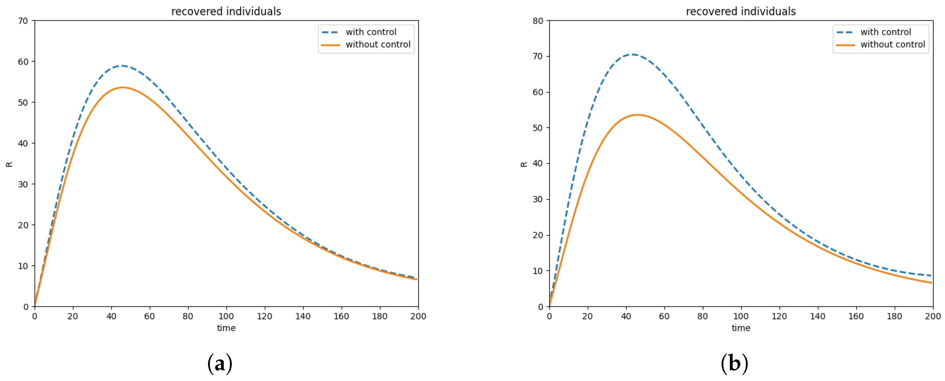
6.2. Optimal Control

In order to obtain the optimal solution path of the system, we adopt the forward–backward sweep method [34]. Here, the forward technique of state variables and the backward technique of adjoint variables are solved using the fourth-order Runge–Kutta method. We take a time interval of [0, 200] for numerical approximation; that is, after 200 days, all controls will stop. The model’s parameters are defined as follows: $\mathrm{\Lambda }=1$, ${\beta }_1=0.4$, ${\beta }_2=0.2$, ${\epsilon }_1=0.2$, ${\epsilon }_2=0.3$, $\theta =0.1$, ${\gamma }_1=0.3$, ${\gamma }_2=0.4$, $\delta =0.2$, $r_1=0.2$, $r_2=0.2$, ${\alpha }_1=0.1$, ${\alpha }_2=0.1$, ${\mu }_1=0.25$, ${\mu }_2=0.4$, and $K=0.1$.

Figure 3a,b show the evolution of infected individuals for both strains $I_1$ and $I_2$. It can be seen that the number of infected individuals in the system with treatment control is much lower than the one without any treatment. These results reveal that the use of treatment control can play a good role in reducing the number of infected individuals and reducing the severity of infection. The text continues here.

Figure 4a shows the changes in recovered individuals. From Figure 4a, we can see that the number of recovered individuals who applied the treatment control increased significantly compared to no treatment at all. This proves that with good treatment, infected people recover more easily than people without any treatment and can easily move out of the category of infection. Figure 4b shows the change in recovered individuals when we increase the cure rate. We can see that when we increase the cure rate, the number of recovered people who add the treatment control increases dramatically. Therefore, it is necessary to add treatment control in case of disease outbreaks.

Finally, Figure 5a,b show the trend plots of optimal control $u_1$ and $u_2$ over time. From Figure 5, it can be seen that during the transmission of infectious diseases, the treatment control of strain-1 remained at the maximum in the first 140 days, and that of strain-2 remained at the maximum in the first 70 days and then gradually decreased until it reaches the lower limit. This phenomenon indicates that in the early stage of the outbreak of the infectious diseases, treatment measures have a significant effect and can effectively prevent the further spread of infectious diseases. Through using the optimal control strategy, effective treatment control can be carried out for the infected individuals. In this way, the number of patients spreading the disease can be reduced, and infectious diseases can be gradually controlled.

7. Conclusions

In this paper, we conducted a study on a deterministic two-strain SEIR model, which uses the saturation treatment function as the optimal control strategy. Our paper is divided into two parts. The first part investigates the global stability of the disease-free equilibrium with fixed control values. In this part, we present the expression of two basic reproduction numbers $R_1$ and $R_2$ associated with our model. Moreover, we defined new thresholds $Z_1$ and $Z_2$ to facilitate the formulation of the results. The result indicate that if $max\{R_1,R_2\}\le min\{1,min\{Z_1,Z_2\}\}$, then the disease-free equilibrium is globally asymptotically stable. In the second part, we investigate the optimal control problem of the model using the optimal control theory and Pontryagin’s maximum principle. Furthermore, we have represented the results in numerical simulations to reveal the influence of treatment control. The results show that optimal treatment reduces the number of infected individuals in both strains $I_1$ and $I_2$, and it increases the number of recovered individuals R after a few days of treatment. This result conveys an important message that the application of treatment control is an effective strategy for controlling the spread of epidemics. The strongest treatment at the beginning of the epidemic can effectively control the spread of the disease. Therefore, in the absence of vaccines or antiviral drugs for the virus, our results suggest that governments should strictly implement treatment strategies to do everything they can to curb the spread of the disease during the pandemic.

In the future, we will expand this work to the fractional scale, coming up with new mathematical models to make it more relevant to real-life infectious diseases. In particular, effective strategies to control and prevent disease will be investigated.

References

1. Jiao, J.; Liu, Z.; Cai, S. Dynamics of an SEIR model with infectivity in incubation period and homestead-isolation on the susceptible. Appl. Math. Lett. 2020, 107, 106442. [Google Scholar] [CrossRef] [PubMed]
2. Lu, G.; Lu, Z. Global asymptotic stability for the SEIRS models with varying total population size. Math. Biosci. 2018, 296, 17–25. [Google Scholar] [CrossRef] [PubMed]
3. Wang, J.-J.; Zhang, J.; Jin, Z. Analysis of an SIR model with bilinear incidence rate. Nonlinear Anal.-Real World Appl. 2010, 11, 2390–2402. [Google Scholar] [CrossRef]
4. Zhou, X.; Guo, Z. Analysis of an influenza A (H1N1) epidemic model with vaccination. Arab. J. Math. 2012, 1, 267–282. [Google Scholar] [CrossRef]
5. Gao, J.; Zhao, M. Stability and bifurcation of an epidemic model with saturated treatment function. In Computing and Intelligent Systems, Proceedings of the ICCIC 2011, Wuhan, China, 17–18 September 2011; Springer: Berlin/Heidelberg, Germany, 2011. [Google Scholar]
6. Ciric, L.; Ume, J.S.; Jesic, S.N. On random coincidence and fixed points for a pair of multivalued and single-valued mappings. J. Inequal. Appl. 2006, 2006, 1–12. [Google Scholar] [CrossRef]
7. Li, J.-Q.; Ma, Z. Stability analysis for SIS epidemic models with vaccination and constant population size. Discrete Contin. Dyn. Syst.-B 2004, 4, 635–642. [Google Scholar] [CrossRef]
8. Iannelli, M.; Martcheva, M.; Li, X. Strain replacement in an epidemic model with super-infection and perfect vaccination. Math. Biosci. 2005, 195, 23–46. [Google Scholar] [CrossRef] [PubMed]
9. Kribs-Zaleta, C.; Velasco-Hernández, J.X. A simple vaccination model with multiple endemic states. Math. Biosci. 2000, 164, 183–201. [Google Scholar] [CrossRef] [PubMed]
10. Wendi, W.; Ma, Z. Global dynamics of an epidemic model with time delay. Nonlinear Anal.-Real World Appl. 2002, 3, 365–373. [Google Scholar] [CrossRef]
11. Kribs-Zaleta, C.; Martcheva, M. Vaccination strategies and backward bifurcation in an age-since-infection structured model. Math. Biosci. 2002, 177–178, 317–332. [Google Scholar] [CrossRef]
12. Kermack, W.O.; McKendrick, Á.G. A contribution to the mathematical theory of epidemics. Proc. Roy. Soc. A 1927, 115, 700–721. [Google Scholar]
13. Rohith, G.; Devika, K.B. Dynamics and control of COVID-19 pandemic with nonlinear incidence rates. Nonlinear Dyn. 2020, 101, 2013–2026. [Google Scholar] [CrossRef] [PubMed]
14. Zhang, Z.; Zeb, A.; Egbelowo, O.F.; Erturk, V.S. Dynamics of a fractional order mathematical model for COVID-19 epidemic. Adv. Differ. Equ. 2020, 2020, 420. [Google Scholar] [CrossRef] [PubMed]
15. Huang, L.; Xia, Y.; Qin, W. Study on SEAI Model of COVID-19 Based on Asymptomatic Infection. Axioms 2024, 13, 309. [Google Scholar] [CrossRef]
16. Xu, C.; Qin, K. Analysis of epidemic situation in novel coronavirus based on SEIR model. Comput. Appl. Softw. 2021, 38, 87–90. [Google Scholar]
17. Khyar, O.; Allali, K. Global dynamics of a multi-strain SEIR epidemic model with general incidence rates: Application to COVID-19 pandemic. Nonlinear Dyn. 2020, 102, 489–509. [Google Scholar] [CrossRef] [PubMed]
18. Meskaf, A.; Khyar, O.; Danane, J.; Allali, K. Global stability analysis of a two-strain epidemic model with non-monotone incidence rates. Chaos Solitons Fractals 2020, 133, 109647. [Google Scholar] [CrossRef]
19. Bhunu, C.P. Mathematical analysis of a three-strain tuberculosis transmission model. Appl. Math. Modell. 2011, 35, 4647–4660. [Google Scholar] [CrossRef]
20. Saha, P.; Ghosh, U. Complex dynamics and control analysis of an epidemic model with non-monotone incidence and saturated treatment. Int. J. Dyn. Control 2022, 11, 301–323. [Google Scholar] [CrossRef]
21. Jana, S.; Nandi, S.K.; Kar, T.K. Complex dynamics of an SIR epidemic model with saturated incidence rate and treatment. Acta Biotheor. 2016, 64, 65–84. [Google Scholar] [CrossRef]
22. Khan, M.A.; Khan, Y.; Islam, S. Complex dynamics of an SEIR epidemic model with saturated incidence rate and treatment. Physica A 2018, 493, 210–227. [Google Scholar] [CrossRef]
23. Saha, P.; Mondal, B.; Ghosh, U. Global dynamics and optimal control of a two-strain epidemic model with non-monotone incidence and saturated treatment. Iran. J. Sci. 2023, 47, 1575–1591. [Google Scholar] [CrossRef]
24. Bentaleb, D.; Harroudi, S.; Amine, S.; Allali, K. Analysis and optimal control of a multistrain SEIR epidemic model with saturated incidence rate and treatment. Differ. Equ. Dyn. Syst. 2020, 31, 907–923. [Google Scholar] [CrossRef]
25. Baba, I.A.; Hıncal, E. Global stability analysis of a two-strain epidemic model with bilinear and non-monotone incidence rates. Eur. Phys. J. Plus 2017, 132, 208. [Google Scholar] [CrossRef]
26. Bentaleb, D.; Amine, S. Lyapunov function and global stability for a two-strain SEIR model with bilinear and non-monotone incidence. Int. J. Biomath. 2019, 12, 1950001. [Google Scholar] [CrossRef]
27. Liu, W.-M.; Levin, S.A.; Iwasa, Y. Influence of nonlinear incidence rates upon the behavior of SIRS epidemiological models. J. Math. Biol. 1986, 23, 187–204. [Google Scholar] [CrossRef] [PubMed]
28. Zhang, X.; Liu, X. Backward bifurcation of an epidemic model with saturated treatment function. J. Math. Anal. Appl. 2008, 348, 433–443. [Google Scholar] [CrossRef]
29. Lakshmikantham, V.; Leela, S.; Martynyuk, A.A. Stability Analysis of Nonlinear Systems; Dekker: New York, NY, USA, 1989. [Google Scholar]
30. van den Driessche, P.; Watmough, J. Reproduction numbers and sub-threshold endemic equilibria for compartmental models of disease transmission. Math. Biosci. 2002, 180, 29–48. [Google Scholar] [CrossRef]
31. Kamrujjaman, M.; Saha, P.; Islam, M.S.; Ghosh, U. Dynamics of SEIR model: A case study of COVID-19 in Italy. Results Control Optim. 2020, 7, 2666–7207. [Google Scholar] [CrossRef]
32. ellman, R.; Pontryagin, L.S.; Boltyanskii, V.G.; Gamkrelidze, R.V.; Mischenko, E.F. Mathematical Theory of Optimal Processes. 1962. Available online: https://api.semanticscholar.org/CorpusID:118166571 (accessed on 1 August 2024).
33. Berhe, H.W.; Makinde, O.D.; Theuri, D.M. Parameter estimation and sensitivity analysis of dysentery diarrhea epidemic model. J. Appl. Math. 2019, 2019, 8465747. [Google Scholar] [CrossRef]
34. Rodrigues, H.S.; Monteiro, M.T.; Torres, D. Optimal control and numerical software: An overview. arXiv 2014, arXiv:1401.7279. [Google Scholar]
Figure 1. Flow chart of SEIR multi-strain problem with treatment.
Mathematics 12 03026 g001
Figure 2. (a) Correlation between R 1 and parameters; (b) correlation between R 2 and parameters.
Mathematics 12 03026 g002
Figure 3. (a) Comparison of strain-1 infected individuals in both systems with and without control; (b) comparison of strain-2 infected individuals in both systems with and without control.
Mathematics 12 03026 g003
Figure 4. (a) Comparison of recovered individuals in both systems with and without control; (b) comparison of recovered individuals in both systems with and without control after increasing treatment rates.
Mathematics 12 03026 g004
Figure 5. (a) The evolution of the optimal control u 1 over time; (b) the evolution of the optimal control u 2 over time.
Mathematics 12 03026 g005