Recurrent Neural Network-Based Model Predictive Control for Continuous Pharmaceutical Manufacturing

Abstract

The pharmaceutical industry has witnessed exponential growth in transforming operations towards continuous manufacturing to increase profitability, reduce waste and extend product ranges. Model predictive control (MPC) can be applied to enable this vision by providing superior regulation of critical quality attributes (CQAs). For MPC, obtaining a workable system model is of fundamental importance, especially if complex process dynamics and reaction kinetics are present. Whilst physics-based models are desirable, obtaining models that are effective and fit-for-purpose may not always be practical, and industries have often relied on data-driven approaches for system identification instead. In this work, we demonstrate the applicability of recurrent neural networks (RNNs) in MPC applications in continuous pharmaceutical manufacturing. RNNs were shown to be especially well-suited for modelling dynamical systems due to their mathematical structure, and their use in system identification has enabled satisfactory closed-loop performance for MPC of a complex reaction in a single continuous-stirred tank reactor (CSTR) for pharmaceutical manufacturing.

1. Introduction

The pharmaceutical industry has shown a growing interest in adopting the concept of continuous manufacturing [1,2] to reduce waste, cost, environmental footprints and lead-times. Coupled with developments in continuous manufacturing technologies and quality by design (QbD) paradigms, there has thus recently been an increasing demand for more advanced system identification and process control strategies for continuous pharmaceutical manufacturing [1].

Continuous manufacturing has the potential of extending the palette of permissible reaction conditions and enabling reaction outcomes that are quite challenging when performed under batch conditions [3,4,5], and its application to the production of complex Active Pharmaceutical Ingredients (APIs) is an emerging research domain. However, the reactions involved are generally both reversible and coupled with many side reactions, which leads to highly non-linear systems that impose difficulties for system identification. The need to operate in tight and extreme conditions also necessitates stricter control requirements [6,7,8]. The complexity of the system, as well as its potential impact on reaction yields, downstream processing requirements and critical quality attributes (CQAs) of final products, render model identification and control of continuous API reactions particularly challenging.

Advanced model-based control technologies promise to improve control of CQAs and are seen as vital to enabling continuous pharmaceutical manufacturing, and their performance hinges on the quality of the model obtained from system identification. Many rigorous physics-based models have been proposed to describe different API reactions [6,9,10] and they have clear physical interpretations. However, these models can suffer from complicated structures and may incur excessive computational costs during online control. The need for models that evaluate quickly for online control purposes is not unique to the pharmaceutical industry, and extensive work has also been done for thin-film deposition in the microelectronics industry [11,12]. Moreover, it may be extremely difficult and expensive to derive accurate models of non-linear systems from first principles in the first place [13]. In contrast, experimental data-driven heuristic models aim to describe underlying processes with relatively simpler mathematical expressions and are thus generally easier to obtain [14]. Neural networks belong to this class of data-driven models, and they have been extensively applied in the chemical and biochemical processing industries, particularly in modelling complex non-linear processes whose process understanding is limited to begin with [15,16,17,18]. The goal of system identification is to create models that capture the relationships between the process state variables and control variables, and data-based empirical models for system identification have been widely studied in previous work [19,20]. Artificial Neural Networks (ANNs) are interesting candidate models for these purposes due to their ability to approximate any continuous function, subject to assumptions on the activation function. RNNs constitute a sub-class of ANNs, and they are structured to use hidden variables as a memory for capturing temporal dependencies between system and control variables. These networks have been extensively used in sequence learning problems like scene labeling [21] and language processing [22], demonstrating good performance. Ref. [23] provides an overview of the neural network applications, particularly from a process systems engineering perspective. In this work, the use of RNNs for system identification of a complex reaction in a single CSTR for pharmaceutical API production will be demonstrated.

The design of effective model-based control algorithms for continuous manufacturing is also a key research focus in academia and industry [24], and the model predictive control (MPC) method is a prominent example that has been widely employed in industrial applications [25,26,27]. It has also been applied in the control of CQAs in continuous pharmaceutical manufacturing [10,24], and an example can be found in [10] where the authors presented two plant-wide end-to-end MPC designs for a continuous pharmaceutical manufacturing pilot plant. This plant covered operations from chemical synthesis to tablet formation, and the MPC designs were obtained using the quadratic dynamic matrix control (QDMC) algorithm. The results showed that, by monitoring the CQAs in real time, critical process parameters (CPPs) could be actively manipulated by feedback control to enable process operation that is more robust and flexible. The advantages that MPC has over conventional proportional-integral-derivative (PID) control are highlighted in [24], which compared their control performance for a feeding blending unit (FBU) used in continuous pharmaceutical manufacturing.

Previous studies have explored the potential of using RNNs with MPC. For example, ref. [28] investigated the use of RNNs in controlling non-linear dynamical systems. RNNs have also been used for predictive control of reactions in CSTRs [29]. However, this CSTR study was limited to relatively simple kinetics like single-step irreversible reactions, i.e., $A\to B$. This paper illustrates therefore how RNNs can be used with MPC of reactions with more complex kinetics.

The paper is organized as follows. Section 2 describes the plant model, which is the subject of system identification, and the control scenarios that will be used to assess closed-loop control performance. Section 3.1 articulates the RNN-based system identification methodology and Section 3.2 describes the MPC problem formulation. Results and discussions are shown in Section 4.

2. Plant Model and Control Scenarios

The following sub-sections describe (i) the true plant model for which system identification will be performed and (ii) the two control scenarios that will be used to assess closed-loop control performance.

2.1. Plant Model

The reaction system comprising of a single CSTR, as was also analysed in [30,31], will be the object of this study. For this work, the focus is on system identification using RNNs with a view towards closed-loop control with MPC, thereby marking a difference from how this reaction system was studied in previous literature. The reaction is described by Equation (1), where A is the feed species, R is the reaction intermediate and the desired product, and S is the undesired by-product:

$$A\underset{{\mathrm{k}}_4}{\overset{{\mathrm{k}}_1}{\rightleftarrows }}R\underset{{\mathrm{k}}_3}{\overset{{\mathrm{k}}_2}{\rightleftarrows }}S$$

(1)

The equations used to represent the dynamical behavior of this system are based on normalized dimensionless quantities and are as shown in Equations (2)–(4) below:

$$\begin{array}{ccc}\hfill \frac{d{C}_A}{dt}& =& q[C_{A0}-C_A]-k_1{C}_A+k_4{C}_R\hfill \end{array}$$

(2)

$$\begin{array}{ccc}\hfill \frac{d{C}_R}{dt}& =& q[1-C_{A0}-C_R]+k_1{C}_A+k_3[1-C_A-C_R]-[k_2+k_4]C_R\hfill \end{array}$$

(3)

$$\begin{array}{ccc}\hfill k_j& =& k_{0,j}exp\left\{{\left[-\frac{E}{R{T}_0}\right]}_j\left[\frac{1}{T}-1\right]\right\},j\in \{1,2,3,4\}\hfill \end{array}$$

(4)

where, $C_{i\in \{A,R,S\}}\in {\mathbb{R}}_{+}$ refers to the species concentration in the reactor, $C_{A0}\in {\mathbb{R}}_{+}$ the feed concentration of A, $q\in {\mathbb{R}}_{+}$ the feed flow rate, and $k_{j\in \{1,2,3,4\}}\in {\mathbb{R}}_{+}$ the rate constants for the respective reaction. For each rate constant, $k_{0,j\in \{1,2,3,4\}}\in {\mathbb{R}}_{+}$ is its associated Arrhenius pre-exponential constant, and ${\left[\frac{E}{R{T}_0}\right]}_{j\in \{1,2,3,4\}}\in \mathbb{R}$ its associated normalised activation energy.

The reactions are first-order and reversible. The reactor is operated isothermally and perfect mixing is assumed. All reactor concentrations are measured in this example. The manipulated variables are q and T, and their values are also measured. It is also assumed that the only species entering the CSTR are A and R, such that their feed concentrations sum up to unity. As such, $C_S$ is easily calculable as a function of time. The values of $k_{0,j\in \{1,2,3,4\}}$ and ${[\frac{E}{R{T}_0}]}_{j\in \{1,2,3,4\}}$ can be found in [31] and are reproduced in the Appendix A for ease of reference.

Figure 1 shows that, at steady-state conditions for a given q, $C_R$ reaches a maximum at a certain temperature, beyond which the reaction gets driven back to the left of Equation (1) to eventually yield only A and no R. This system possesses rich and relevant dynamics for continuous pharmaceutical manufacturing and is therefore worth detailed investigation.

The control problem for this system is challenging due to the existence of input multiplicities [30,32], which occur when a set of outputs can be reached by more than one set of inputs. This implies the existence of sign changes in the determinant of the steady-state gain matrix within the operating region. Linear controllers with integral action therefore become unstable for this problem.

In what follows, as is common in digital control, the discrete-time domain with time-steps denoted by $k\in {\mathbb{Z}}_{+}$ will be used. The state vector, x, and manipulated vector (MV), u, are also defined as follows: $x\triangleq {[C_A,C_R]}^{\prime }$, $u\triangleq {[q,T]}^{\prime }$. The underlying plant model can therefore be described by a non-linear discrete-time difference equation, as Equations (5) and (6) show:

$$\begin{array}{ccc}\hfill x_{k+1}& =& \mathsf{\Phi }(x_k,u_k)\hfill \end{array}$$

(5)

$$\begin{array}{ccc}\hfill y_k& =& x_k\hfill \end{array}$$

(6)

where $k\in {\mathbb{Z}}_{+}$ is the discrete-time index, and $x_k$ and $u_k$ the state vector and manipulated vector at time-step k respectively. $\mathsf{\Phi }$(.) is the state-transition equation consistent with Equations (2)–(4), and full state feedback is assumed, such that the measured output $y_k$ equals $x_k$ for all time-steps.

The system identification problem consists of finding an approximation of Equations (2)–(4), and forms the subject of Section 3.1 in this paper. It will be supposed that the $p-$step ahead prediction problem is of vital interest for MPC. Throughout this paper, all problems are considered from time-step zero, and a sampling time $\Delta t$, of $0.1$ time units is used.

2.2. Closed-Loop Control Scenarios

The approach taken to construct the RNN for MPC is to train the RNN with data from the training set, then evaluate the model performance using previously unseen data from the test set. However, since the main focus of this study is process control, the final evaluation will be performed by comparing the closed-loop performance of the RNN-based MPC (RNN-MPC) against a benchmark non-linear MPC (NMPC) controller that directly uses the true plant model, as described in Equations (2)–(4), as its internal model.

Two control scenarios were selected for performance evaluation and the operating conditions for each scenario are reflected in the first two rows of

Table 1. Initial conditions and set-points for control scenarios.

Control Scenario	${\mathit{C}}_{\mathit{A}}$	${\mathit{C}}_{\mathit{R}}$	q	T
I: Start-up	0.692	0.287	0.800	0.800
II: Upset-recovery	0.822	0.152	0.800	1.100
Set-point (maximum $C_R/C_A$)	0.324	0.406	0.800	1.043

. These scenarios are namely cases I and II, and they correspond respectively to a reactor system start-up case and an upset-recovery case. In case I, the system is assumed to initially be at a low temperature state with a relatively low product concentration. In case II, the initial conditions correspond instead to a high-temperature and low-yield state. Figure 2 shows the locations of the initial conditions for these control scenarios with respect to the set-point, with case I represented by the purple point to the left of the peak in the green $C_R$ plot, and case II represented by the cyan point to the right of the same peak.

The set-point is judiciously located where the ratio of the product concentration to the feed concentration, $C_R/C_A$, is maximised. This set-point corresponds to a product concentration that is slightly lower than what is maximally achievable. The rationale for choosing this set-point over the point for maximum $C_R$ is that it maximizes yield whilst minimising downstream separations cost. The operating conditions corresponding to the target set-point are shown in the last row of Table 1.

3. Methodology

3.1. Non-Linear Time-Series System Identification via Recurrent Neural Networks

ANNs serve as a potential source of models that capture the dynamics of highly non-linear systems sufficiently well while being relatively easy to obtain and evaluate online, and RNNs are a sub-class of ANNs that are structured to better capture temporal dependencies in the system. RNNs are particularly useful for making p-step ahead predictions of state variables for predictive control, because the prediction for time-step p depends on the present state and all control actions in time-step $k\in \{0,\dots ,p-1\}$. The prediction for time-step $p-1$ used in the above prediction for time-step p depends similarly on the present state and all control actions in time-step $k\in \{0,\dots ,p-2\}$, and so on.

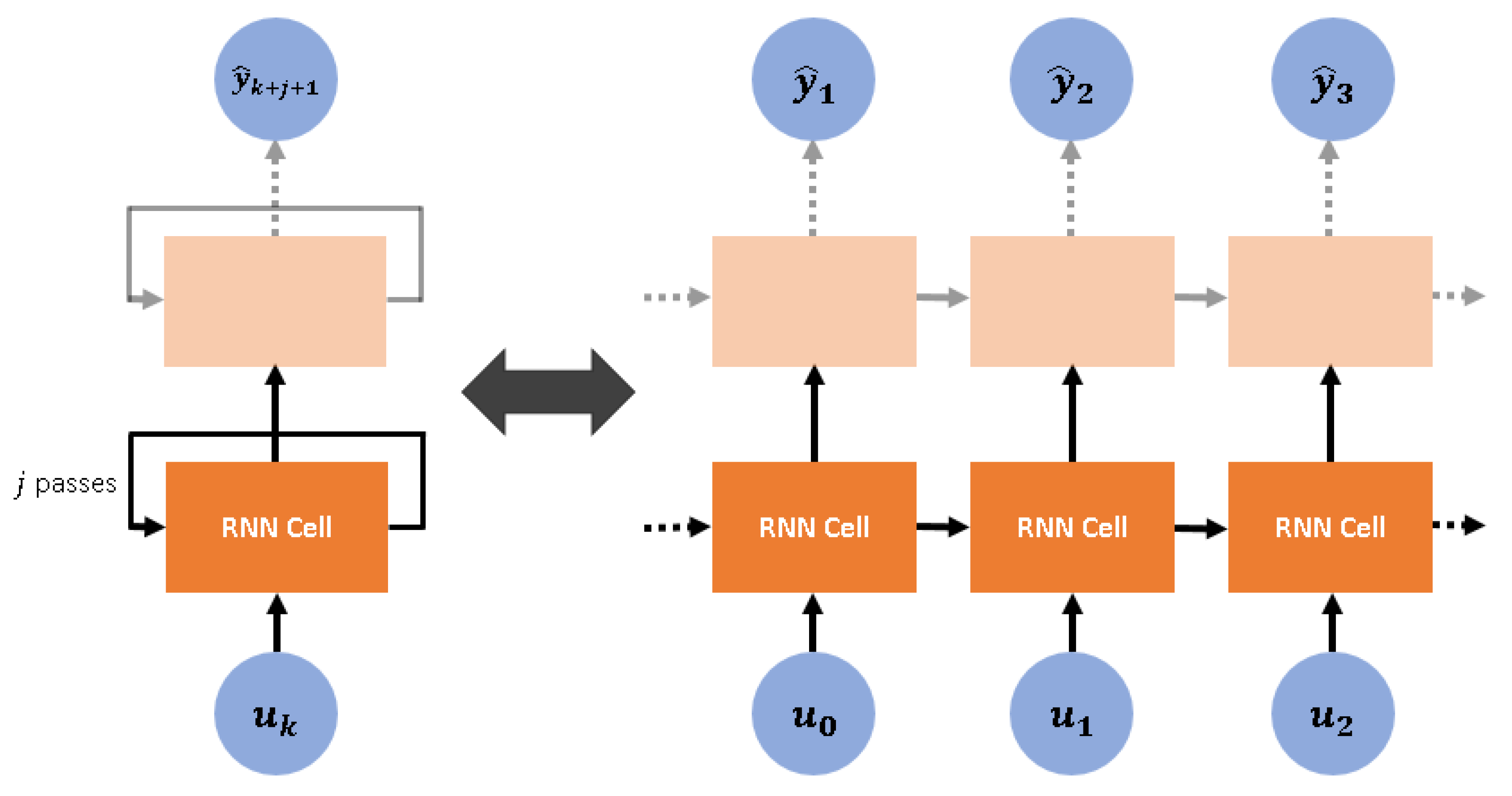
Figure 3 illustrates the structure of an RNN layer in its compact and unfolded forms. The unfolded form reveals the repeating cells forming each layer, and each cell is taken in this study to represent a time-step, such that the state of the cell representing time-step $k\in \{0,\dots ,p-1\}$ serves as the input for a cell representing time-step $k+1$. Each cell contains N number of hidden nodes that encode the state representation, where N is user-specifiable. The equations that mathematically characterise a single RNN cell in a single-layer RNN are as shown in Equations (7) and (8) below:

$$\begin{array}{ccc}\hfill h_k& =& W_{h,h}{h}_{k-1}+W_{u,h}{u}_{k-1}+b_1\hfill \end{array}$$

(7)

$$\begin{array}{ccc}\hfill {\widehat{y}}_k& =& \mathsf{\Phi }(h_k+b_2)\hfill \end{array}$$

(8)

where $k\in \{1,\dots ,p\}$ is the discrete-time index with p the prediction horizon, $h_k\in {\mathbb{R}}^N$ the (hidden) state of the cell representing time-step k, $u_{k-1}\in {\mathbb{R}}^2$ the cell input, ${\widehat{y}}_k\in {\mathbb{R}}^2$ the cell output which corresponds to the state vector prediction for time-step k, $(b_1,b_2)\in {\left({\mathbb{R}}^N\right)}^2$ the offset vectors, $W_{u,h}\in {\mathbb{R}}^{N\times 2}$ and $W_{h,h}\in {\mathbb{R}}^{N\times N}$ the input-to-hidden-state weight matrix and the hidden-state-to-hidden-state weight matrix respectively, and $\mathsf{\Phi }:{\mathbb{R}}^N\to {\mathbb{R}}^2$ an activation function that is applied element-wise. $h_0$ is initialised in this study by using $y_0$.

Equations (7) and (8) are generalisable to deep RNNs containing more than one layer. For an l-layer RNN, the activation functions for layers $j\in \{2,\dots ,l\}$ take the form $\mathsf{\Phi }:{\mathbb{R}}^N\to {\mathbb{R}}^N$, and the input-to-hidden-state weight matrices have dimensions $N\times N$ instead. Deep RNNs may be preferred to single-layer RNNs for their enhanced ability to learn features of the dynamical system that occur “hierarchically”, but this comes at the expense of longer RNN training times stemming from more parameters to train.

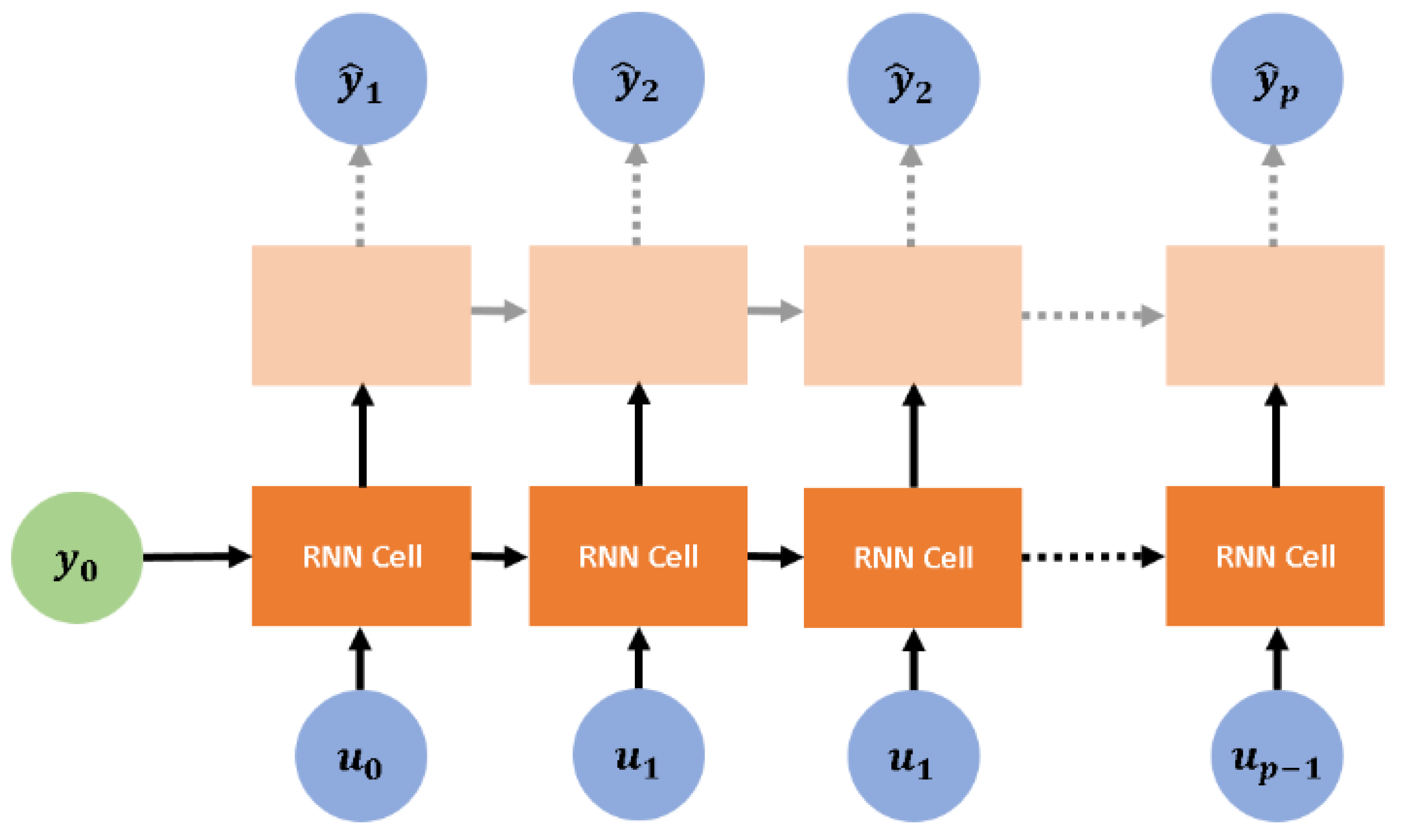
The regressors required to predict ${\widehat{y}}_{k\in \{1,\dots ,p\}}$ are henceforth represented by ${\varphi }_k:=\{y_0,u_0,\dots ,u_{k-1}\}$, and they are introduced into the RNN in a fashion illustrated in Figure 4. Equation (9) below serves as a shorthand to describe the RNN:

$$\begin{array}{ccc}\hfill {\widehat{y}}_k& =& {\widehat{f}}_{RNN}\left({\varphi }_k\right),k\in \{1,\dots ,p\}\hfill \end{array}$$

(9)

An RNN is characterised by the values of $W_{h,h}$, $W_{u,h}$, $b_1$ and $b_2$ for all layers, and these values constitute the set of parameters. These parameters are learnt from training data by minimising the predictive error of the model on the training set as determined through a user-specified loss function. The learning process is performed through the back-propagation through time (BPTT) algorithm that estimates the gradient of the loss function as a function of the weights, and an optimisation algorithm that uses the calculated gradient to adjust the existing weights. The adaptive moment estimation algorithm (Adam) [33] is an example of an optimisation algorithm that is widely used.

The RNN parameters may be difficult to train in some cases due to problems with vanishing and exploding gradients, and RNN cells with different structures can be used to circumvent this issue. Long Short-Term Memory cells (LSTMs) were developed to address these problems, and they are used as the repeating cell in this study. Further details on LSTM cells may be found in the Appendix B.

To generate the data set for training the RNNs in this study, a numerical model of the CSTR system based on Equations (2)–(4) is needed, because this data consists precisely of this system’s response to MV perturbations. This numerical model was implemented in Python version 3.6.5, and its temporal evolution between sampling points was simulated using the explicit Runge-Kutta method of order 5(4) through the scipy.integrate.solve_ivp function.

MV perturbations are then introduced into the system to obtain its dynamic response. This procedure mimics the manual perturbation of the system through experiments, which become necessary in more complicated reaction systems whose reaction kinetics and overall dynamics resist expression in neat analytical forms. These perturbations take the form of pre-defined sequences of control actions, ${\left\{u_{\exp ,k}\right\}}_{k\in \{0,\dots ,T_e-1\}}$, where the “exp” subscript refers to “experiment” and $T_e$ represents the final time-step for the experiment. These control actions are separated by $\Delta t$.

To simulate the system’s dynamic response to the experimental sequence, the control actions associated to the element in this sequence, $u_{\exp ,k}={[q_{\exp ,k},T_{\exp ,k}]}^{\prime }$, $k\in \{0,\dots ,T_e-1\}$, are applied at time-step k for a period of $\Delta t$, during which the system’s evolution with this MV is simulated using the Runge-Kutta method of order 5(4). Once $\Delta t$ elapses, $u_{\exp ,k+1}$ is applied with the system evolution proceeding in the same manner. This procedure repeats until the final time-step, $T_e$, is completed.

A history of the system’s experimental dynamic response is associated to each experimental sequence, which takes the form of ${\left\{y_{\exp ,k}\right\}}_{k\in \{1,\dots ,T_e\}}$. $y_{\exp ,k}$ is the measured system output at time-step k after $u_{\exp ,k-1}$ has been applied to the system for a period of $\Delta t$. This history corresponds to the labels in machine learning terminology, and the data set is thereafter constructed from both the experimental sequences and their associated labels. For the p-step ahead prediction problem, each data point thus takes the form $\{y_k,u_k,u_{k+1},\dots ,u_{k+p-1}\}$ with the associated label $\{y_{k+1},\dots ,y_{k+p}\}$, $k\in \{0,\dots ,T_e-p\}$. 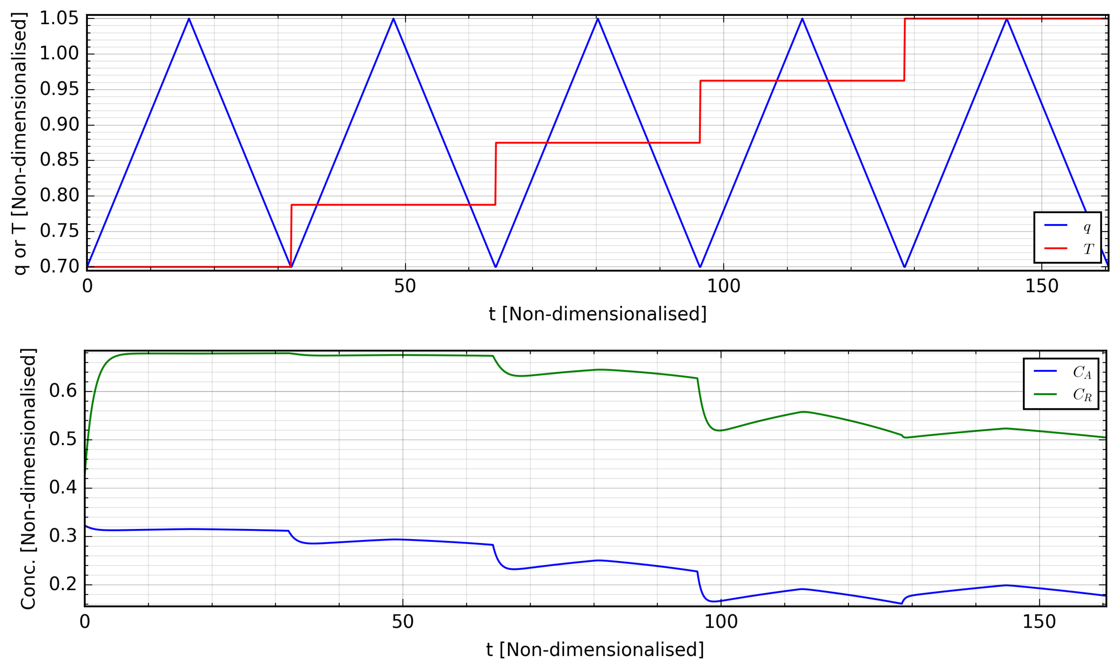$T_e-p$ data points can thus be extracted from each experimental sequence. Multiple experimental sequences can be constructed by perturbing the MVs in different ways, and such a sequence is shown in Figure 5 with its associated system dynamical response, with this sequence showing variations of q in the range $[0.70,1.05]$ for fixed values of T. For this study, these sequences were generated in a fashion similar to Figure 5, by introducing linear changes of different frequencies to one component of the MV spanning its experimental range while keeping the other MV component constant.

Before training the RNNs, it is necessary to split the data set into the training set and the test set. The training set contains the data with which the RNN trains its weight matrices, and the test set will be used to determine the models with the best hyperparameters. The two hyperparameters considered in this study are the number of hidden nodes, which also correspond to the dimensionality of the hidden states, and the number of hidden layers.

The experimental simulations and the extraction of training data were performed using Python version 3.6.5 for this study. Keras version 2.1.5, an open-source neural network library written in Python, was used for RNN training with TensorFlow version 1.7.0 as its backend.

3.2. Control Problem Formulation

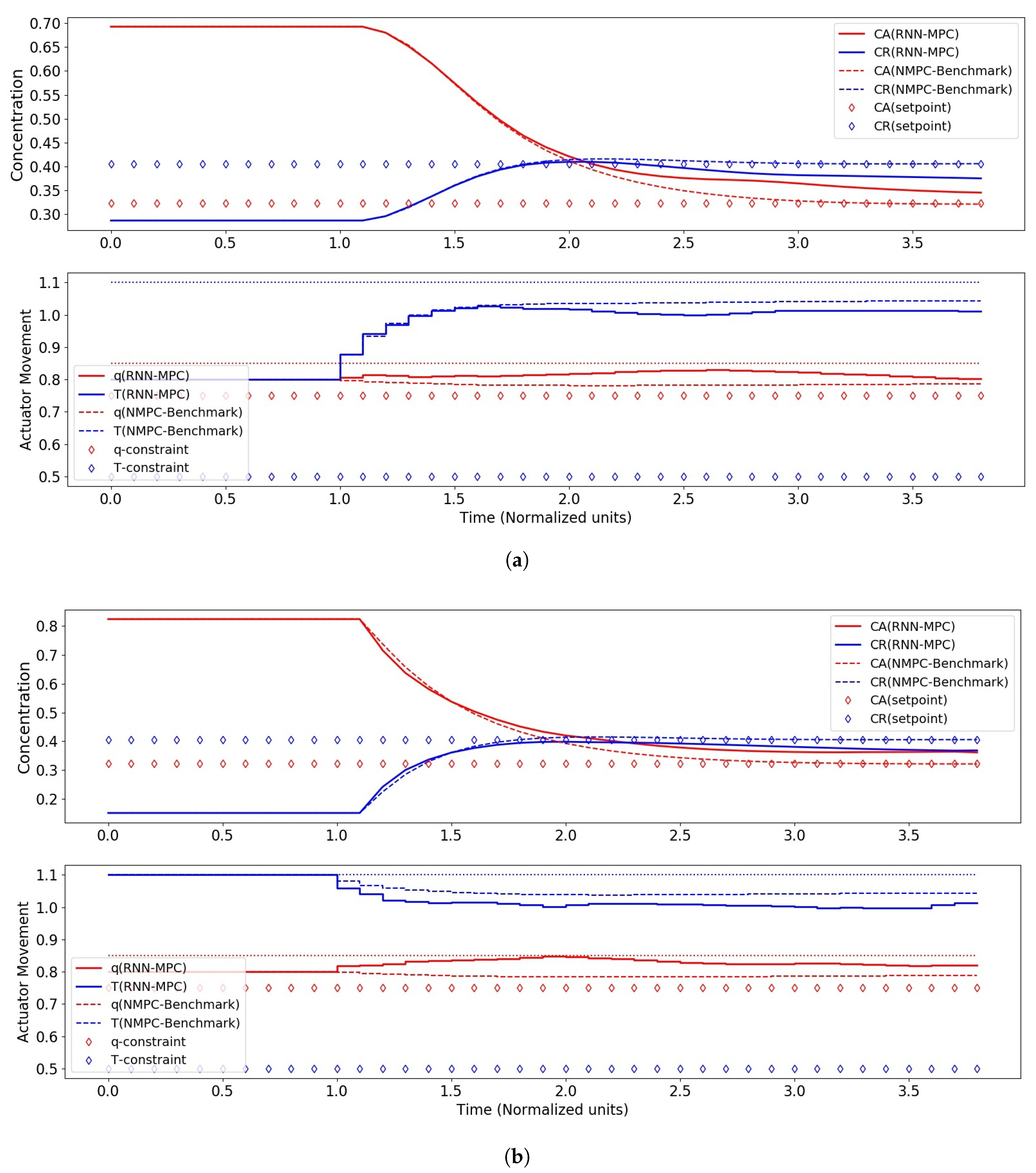
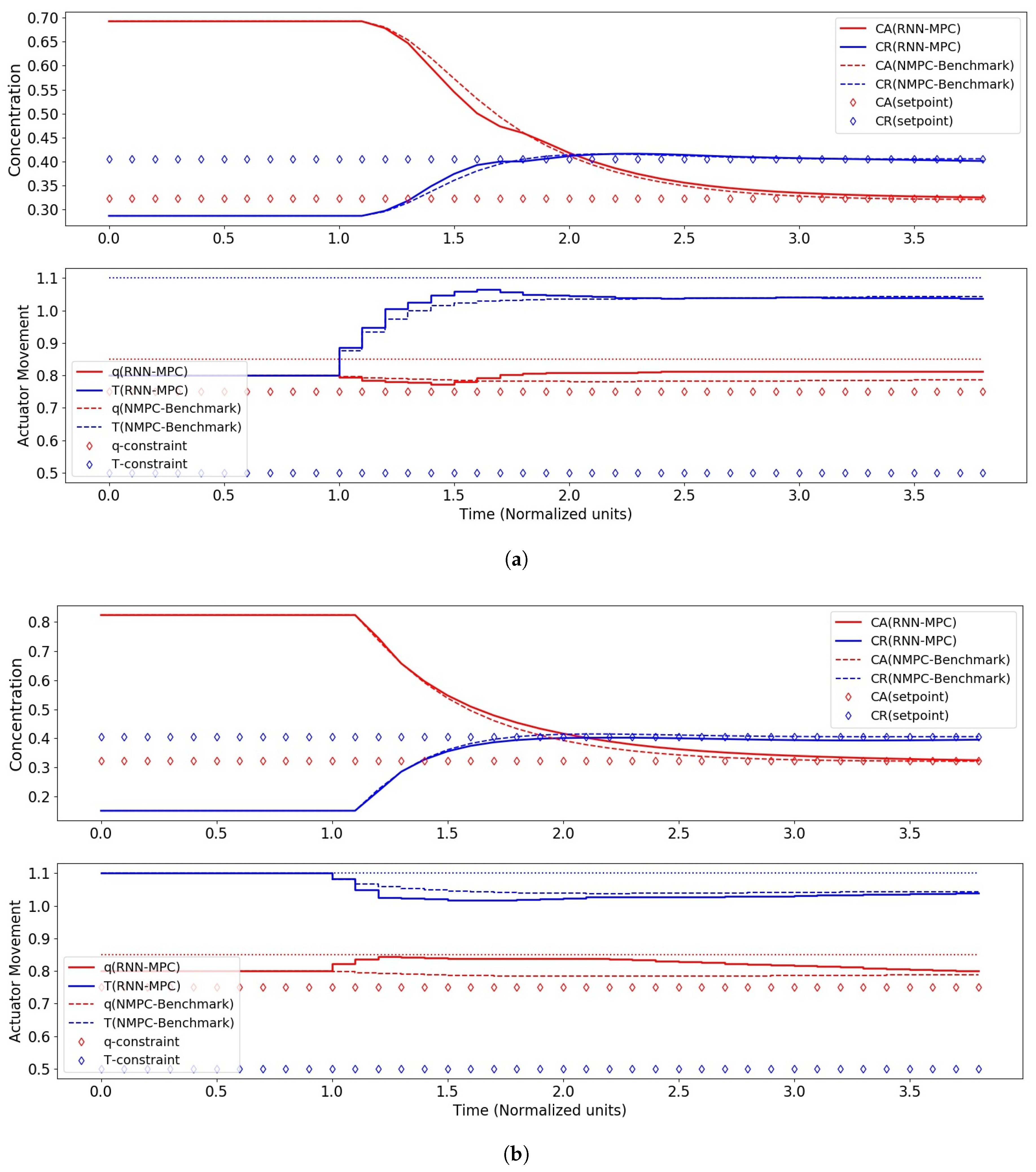
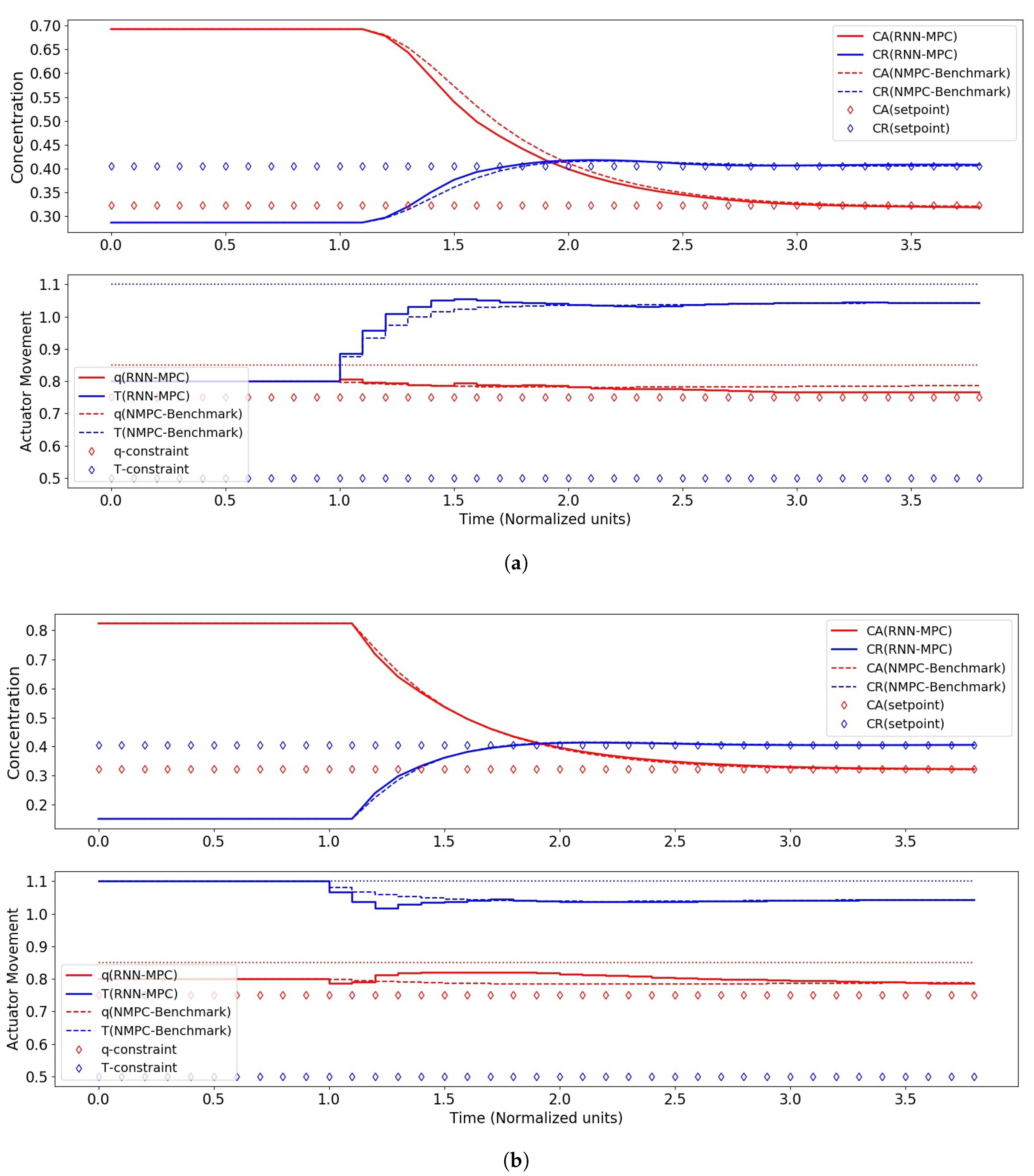
MPC is a control strategy that selects a set of m future control moves, $\{u_0,\dots u_{m-1}\}$, that minimises a cost function over a prediction of p steps by incorporating predictions of the dynamical system for these p steps, $\{{\widehat{y}}_1,\dots ,{\widehat{y}}_p\}$. The cost function is typically chosen to punish large control actions, which implies greater actuator power consumption, and differences between the state vector and the set-point at each time-step. Input and output constraints can also be factored into the MPC formulation. Since MPC performance depends on the quality of the predictions of the system, obtaining a reasonably accurate model through system identification is crucial.

The MPC problem can be formulated as shown in Equations (10)–(13) below:

$$\begin{array}{c}\underset{\{\Delta u_0,\Delta u_1,\dots ,\Delta u_{m-1}\}}{min}\left\{\sum _{k=1}^p{({\widehat{y}}_k-y_k^{*})}^{\prime }{Q}_y({\widehat{y}}_k-y_k^{*})+\sum _{k=0}^{m-1}\Delta u_k^{\prime }{Q}_u\Delta u_k\right\}\mathrm{s}.\mathrm{t}.\end{array}$$

(10)

$$\begin{array}{c}{\widehat{y}}_k={\widehat{f}}_{RNN}\left({\varphi }_k\right),k\in \{1,\dots ,p\}\end{array}$$

(11)

$$\begin{array}{c}{u}_k\in [u_{\min ,k},u_{\max ,k}],k\in \{0,\dots ,m-1\}\end{array}$$

(12)

$$\begin{array}{c}\Delta u_k\in [\Delta u_{\min ,k},\Delta u_{\max ,k}],k\in \{0,\dots ,m-1\}\end{array}$$

(13)

where $p\in {\mathbb{Z}}_{+}$ is the prediction horizon, $m\in \{1,\dots ,p\}$ the control horizon, ${\widehat{y}}_k\in {\mathbb{R}}^2$ the prediction of the state vector for the discrete-time step k obtained from the RNN, ${\widehat{f}}_{RNN}$ described in Equation (9), $y_k^{*}\in {\mathbb{R}}^2$ the set-point at time-step k, $u_k\in {\mathbb{R}}^2$ the MV for time-step k, $\Delta u_k\triangleq u_k-u_{k-1}$ the discrete-time rate of change of the MV which corresponds to the control action size at time-step k, $(Q_y,Q_u)\in {\left({\mathbb{R}}^{2\times 2}\right)}^2$ symmetric positive semi-definite weight matrices, and $(u_{\min ,k},u_{\max ,k},\Delta u_{\min ,k},\Delta u_{\max ,k})\in {\left({\mathbb{R}}^2\right)}^4$ the lower and upper bounds for the control action and the rate of change of the control action at time-step k. In the above formulation, it is assumed that there are no changes in actuator position beyond time-step $m-1$, i.e., $\Delta u_{m-1}=\Delta u_{m+k}=0,k\in \{0,\dots ,p-m-1\}$.

This optimization problem is not convex in general and thus does not possess special structures amenable to global optimality. This is therefore a Non-Linear Programming (NLP) problem, and modern off-the-shelf solvers can be used to solve it. This problem is solved at every time-step to yield the optimal control sequence for that time-step, $\{\Delta u_0^{*},\dots ,\Delta u_{m-1}^{*}\}$. The first element, $\Delta u_0^{*}$, is then applied to the system until the next sampling instant, where the problem is solved again to yield another optimal control sequence. This procedure is then repeated in a moving horizon fashion.

The MPC controller in this study was implemented in Python version 3.6.5 through the scipy.optimize.minimize function, and the sequential least squares quadratic programming (SLSQP) algorithm was selected as the option for this solver.

4. Results and Discussion

The RNN-MPC workflow consists of (i) gathering experimental sequence data with perturbations of the MV to generate the data set; (ii) learning the RNNs from the training set and validating their performance with test data, and selecting the RNNs with the best test performance; and (iii) integrating the chosen RNN with the MPC and finally evaluating its control performance.

4.1. System Identification

RNNs with 250, 500 and 1000 hidden nodes were trained for this study, and the number of RNN layers for these models was also varied from 1 to 3. The validation performance of these models on the test set was quantified through the root-mean-square error (RMSE) metric, which is defined as shown in Equation (14) below:

$$\begin{array}{ccc}\hfill \mathrm{RMSE}& =& \sqrt{\left(\frac{1}{N_{\mathrm{test}}}\sum _{i=1}^{N_{\mathrm{test}}}\sum _{j=1}^p{\left({\left({\widehat{y}}_j\right)}_i-{\left(y_{\exp ,j}\right)}_i\right)}^2\right)}\hfill \end{array}$$

(14)

where $N_{\mathrm{test}}\in {\mathbb{Z}}_{+}$ is the number of data points in the test set, $p\in {\mathbb{Z}}_{+}$ the prediction horizon, ${\left({\widehat{y}}_j\right)}_i\in {\mathbb{R}}^2$ the j-ahead output prediction for data point i, and ${\left(y_{\exp ,j}\right)}_i\in {\mathbb{R}}^2$ the corresponding experimentally-determined output which also represents the ground truth that predictions are tested against. The smaller the RMSE of the model on the test data, the better its general predictive power.

Table 2. Root-mean-square error (RMSE) over test data of RNNs trained over 1000 epochs.

No. Layers / No. Nodes	250	500	1000
1	0.0299	0.0268	0.0206
2	0.0238	0.0118	0.0083
3	0.0262	0.0119	0.0125

tabulates the validation performance of the RNNs on the test data, and it can be observed that prediction performance improves with an increasing number of hidden nodes. This is because hidden states of greater dimensionalities offer greater latitude for capturing more features of the underlying system, contributing to its temporal dynamics. An improvement of the validation performance can also be observed with an increase of the number of hidden layers from 1 to 2. This observation is attributable to the potential of deep hierarchical models to better represent some functions than shallower models [34].

However, performance deteriorated when the number of layers was increased from 2 to 3, and this may be due to the additional layers introducing more model parameters that needed to be tuned, such that the training data set became too small to tune all of them correctly.

Table 2 reveals that RNNs with two hidden layers and 1000 hidden nodes for each RNN cell gave the best validation performance over the test set, with this representing the optimised hyperparameter configuration. An RNN with two hidden layers and 2000 hidden nodes was also trained and it was observed that performance deteriorated when even more hidden nodes were used. This result is tabulated in

Table 3. RMSE over test data of RNNs with hidden layers and either 1000 or 2000 nodes trained over 1000 epochs.

No. Layers	No. Nodes	RMSE
2	1000	0.0083
2	2000	0.0177

, and possible explanations may be that the 2000-node network overfitted the training data, or that the use of 2000-node cells introduced more parameters to the model, rendering the existing training data set too small to tune the additional parameters correctly. RNN with two hidden layers will be used for subsequent closed-loop control studies.

It is also worth noting that validation performance is also a function of the quality of the training set. This performance can be further improved by using a larger training set reflecting the system dynamics within the control range, particularly for any control scenarios earmarked as important.

The prediction performances of this optimised RNN on the training and test sets are respectively shown in Figure 6 below for completeness.

Figure 6a reveals a good fit of the RNN to the training data, and testifies to the model’s ability to reflect highly dynamic outputs from highly dynamic training data. Figure 6b shows that the model succeeded in capturing the general trends for previously unseen test data. Even though this fit was not perfect, particularly for $C_R$ between 3 and 4 time units, it will be demonstrated in a later section that satisfactory closed-loop performance can still be achieved with predictions from this RNN.

4.2. RNN-MPC Closed-Loop Control Performance

As described in Section 2.2, the objective in both control scenarios is to bring the system quickly and smoothly to a target set-point where the ratio of $C_R$ to $C_A$ is maximised, because this maximises yield while minimising downstream separations cost. Since MPC strategies based on single linear models do not perform well for this example [32], non-linear MPC solutions will be required.

The MPC formulation was shown in Equations (10)–(13), and the prediction and control horizons for the MPC controller implemented for this study were set to 10 for both control scenarios, i.e., $p=m=10$. Since the sampling rate, $\Delta t$, was set as 0.1 time units, p and m correspond to 1.0 time unit. The total simulation time, $N_{\mathrm{sim}}$, was set to 40, corresponding to 4.0 time units. The weight matrices for the controller, $Q_y$ and $Q_u$, were defined as $\mathrm{diag}[2.4,5.67]$ and $\mathrm{diag}[25,25]$ respectively. The coefficients selected for $Q_y$ reflect that controlling $C_R$ is more important than controlling $C_A$, and $Q_u$ contain coefficients that are even larger to avoid control actions that are over-aggressive, since these control actions cause system instability. For the constraints, $[u_{\min ,k},u_{\max ,k}]=[{[0.75,0.5]}^{\prime },{[0.85,1.1]}^{\prime }]$, $\forall k\in \{0,N_{\mathrm{sim}-1}\}$ and $[\Delta u_{\min ,k},\Delta u_{\max ,k}]=[{[-0.1,-0.1]}^{\prime },{[0.1,0.1]}^{\prime }]$, $\forall k\in \{0,N_{\mathrm{sim}-1}\}$.

In what follows, the closed-loop control performance of the RNN-MPC controller will be benchmarked against the NMPC controller whose internal model is the actual full plant model as described in Equations (2)–(4). This NMPC controller was implemented using the same software as that of the RNN-MPC controller, whose implementation was described in Section 3.2.

The indices used to evaluate control performance are defined as shown in Equations (15) and (16) below:

$$\begin{array}{c}J=\sum _{k=1}^{N_{\mathrm{sim}}}\left({(y_k-y_k^{*})}^{\prime }{Q}_y(y_k-y_k^{*})+\Delta u_k^{\prime }{Q}_u\Delta u_k\right)\end{array}$$

(15)

$$\begin{array}{c}\mathcal{I}=\left(1-\frac{J_{\mathrm{RNN}}-J_{\mathrm{NMPC}}}{J_{\mathrm{NMPC}}}\right)\times 100\%\end{array}$$

(16)

where $y_{k\in \{1,\dots ,N_{\mathrm{sim}}\}}\in {\mathbb{R}}^2$ and $y_{k\in \{1,\dots ,N_{\mathrm{sim}}\}}^{*}\in {\mathbb{R}}^2$ are the measured output and the set-point at time-step k respectively, $\Delta u_k\in {\mathbb{R}}^2$ the size of the control action at time-step k, and $(Q_y,Q_u)\in {\left({\mathbb{R}}^{2\times 2}\right)}^2$ the symmetric positive semi-definite weight matrices.

Figure 7, Figure 8, Figure 9 and Figure 10 below show the performance of the RNN-MPC and NMPC controllers on both control scenarios for 250, 500, 1000 and 2000 hidden nodes respectively.

Table 4. Performance of closed-loop RNN-MPC as a function of RNN nodes (two layers).

No. Nodes	Average Performance Index,${\mathcal{I}}_{\mathrm{avg}}$	Comments
250	93.7	Steady-state Offset
500	95.8	Steady-state Offset
1000	100.0	Desired Performance
2000	98.6	Steady-state Offset

tabulates the performance index averaged over both control scenarios for each RNN-MPC controller for the same set of values for the number of hidden nodes.

The results show that the RNN-MPC controllers exhibited stability even with only 250 hidden nodes for both control scenarios, suggesting a robustness associated with the RNN-MPC combination.

For the RNN-MPC controller with 250 hidden nodes, while the NMPC controller exhibited no steady-state offset, this RNN-MPC controller showed significant steady-state offsets for both control scenarios. However, the initial transient response of the system under RNN-MPC control was similar to its NMPC benchmark for both scenarios, suggesting that the RNN succeeded in capturing the global dynamics of the system, and that 250 nodes may have not been sufficient for the model to learn the subtler dynamics that would have allowed the controller to bring the system precisely back to the set-point. A notable improvement in performance was observed with 500 nodes, although steady-state offsets remained for both scenarios.

The best closed-loop control performance was obtained with 1000 nodes, and this is consistent with the finding that this RNN had the best validation performance on the test data. The control performance of this RNN-MPC was in fact comparable to its NMPC counterpart, with an ${\mathcal{I}}_{\mathrm{avg}}$ of 100.0. For 2000 nodes, a deterioration of control performance could be seen with the reappearance of the steady-state offsets for both scenarios, and this may be attributable to the RNN’s poorer validation performance on the test data.

To assess the temporal performance of the RNN-MPC controller, 1000 model inputs were generated randomly and the average computational times required by the NMPC and the RNN-MPC controllers to generate a single prediction for use in the optimiser are tabulated in

Table 5. Time required to generate a single prediction averaged over 1000 predictions.

	NMPC	RNN-MPC
Time required	1.55 ms	1.17 ms

. The RNN for this temporal benchmarking has 1000 hidden nodes and two layers, and the NMPC generates predictions by using the Runge-Kutta method of order 5(4) to march the system forward in time. The predictions for both controllers were generated on an Intel(R) Xeon(R) CPU E5-1650 with 16 GB RAM.

The results in Table 5 show that, for the simulation context described in the previous paragraph, the times required by the internal models of both controllers to generate a single prediction are of the same order of magnitude, with the RNN even outperforming its NMPC counterpart slightly. This testifies to the RNNs being a model that can generate predictions for MPC control at least as fast as the true plant model for this CSTR system.

This CSTR system is a comparatively simple dynamical system, and other systems can have more complex exact representations whose evaluation for prediction purposes may take a considerably longer time. Even though these models generate very good predictions, they would be too slow to evaluate to be useful for online control. Having observed from earlier discussions that stable control performance can be achieved if the RNN succeeds in capturing the global dynamics, imperfect predictions may in fact be tolerable if it entails an RNN that is easier to train and faster to evaluate. RNNs can therefore serve to balance the needs of MPC for good and quick predictions.

To summarise, even if the system identification by the RNNs does not perfectly describe the underlying plant dynamics, stable closed-loop control performance can be achieved as long as the global dynamics of the system are captured. Further refinements to the RNN can be made by optimising its hyperparameters, which in this study have been selected to be the number of hidden nodes and hidden layers, to obtain a configuration that is capable of capturing the subtler dynamics of the system while avoiding overfitting on the training set.

5. Conclusions and Future Research

In this study, a multiple-input multiple-output CSTR that houses a reaction exhibiting output dynamics was studied. The methods for generating the control-oriented RNNs and integrating their use into MPC controllers were articulated, and the performance of the RNN-MPC controllers was benchmarked against NMPC controllers that used the true plant model directly as its internal model.

Two control scenarios were simulated, one involving reactor start-up and the other involving upset-recovery, and the results showed that even if the RNNs do not perfectly describe the underlying plant dynamics, RNN-MPC controllers can give stable closed-loop control performance for these scenarios as long as the global dynamics of the system are captured. These RNNs can be refined through hyperparameter optimisation to obtain configurations that are capable of capturing the subtler dynamics of the system while avoiding overfitting on the training set, further augmenting their effectiveness as control-oriented models for MPC.

It is finally noted again that linear controllers with integral action perform poorly for systems exhibiting input multiplicities, and that rigorous physics-based models like the model used for the benchmark NMPC controller can be difficult to obtain in practice and may be too expensive to evaluate to be useful for online MPC control. The approach presented in this study exploits the ability of RNNs to capture the temporal dynamics of the system, and it was shown that RNN-based system identification methods can give control-oriented models for MPC that offer satisfactory performance for two important control scenarios. As the creation of these RNNs is a data-driven process which yields progressively more effective models with larger amounts of process and sensor data, these models serve indeed as an alternative source of control-oriented models that capture the dynamics of highly non-linear systems sufficiently well while being relatively easy to obtain and evaluate online. This opens promising avenues for the application of RNNs or other ML models in enabling continuous pharmaceutical manufacturing practices.

A potential way to bring this study forward is to compare different ML or RNN architectures for MPC control-oriented system identification. Measurement noise can be incorporated to simulate realistic sampling scenarios and evaluate the robustness to noise of the ML system identification and the ML-MPC control techniques. Cross-validated optimisation of more hyperparameters characterising the ML model, which can potentially include the regular dropout rates between hidden layers, the learning rates and gradient clipping values among others, as well as a more detailed study of the effects of the experimental sequences on the quality of the ML model trained, can also give future practitioners useful heuristics for creating and tuning MLs for their own purposes.

Future research can also involve extending the methodology to multiple CSTRs, and to reaction kinetics of increasing complexity and of more immediate relevance to the pharmaceutical industry. These can be done in view of an eventual real-world implementation of these RNN-MPC or ML-MPC control strategies, from which further comparisons of these controllers to conventional PID controllers, and other MPC strategies like linear MPC and offset-free MPC, can also be made.