1. Introduction
The study of graph invariants or topological indices has been proven to be of crucial importance in various interdisciplinary topics. Generally, the existing known topological indices could be divided into distance-based, degree-based, or structure-based ones; some of the studies on these three categories are referred to in [
1,
2,
3,
4] and the references therein. The number of subtrees, or simply the subtree number, is one of the counting-based graph invariants.
Finding and/or enumerating special topological structures or graph patterns has become an important problem due to their applications including, to name a few, frequent subgraphs mining [
5], network optimization design [
6,
7], and local network reliability [
8,
9]. In particular, the subtree number has also been shown to be correlated to phylogenetic reconstruction [
10] and various chemical indices such as the Wiener index (closely correlated with the boiling point of paraffin [
3]), the Merrifield–Simmons index, and the Hosoya index [
11]. Research results also show that there exists an amazing “negative correlation” between the number of subtrees and the Wiener index [
12,
13,
14,
15,
16,
17]. Therefore, the subtree number index can indirectly characterize the physical–chemical characteristics of molecules.
Various topics related to the subtree number have been explored over the past years, such as extremal problems [
12,
18,
19], the subtree density problem [
20,
21,
22], generic chemical structures storage problems [
23,
24], fault tolerant computing and parallel scheduling [
25,
26], recognition of substructure [
27], simplification of the flow networks [
28], Markovian queuing systems decomposition [
29], and matching problems [
30,
31].
By using “generating functions”, Yan and Yeh [
4] presented a linear-time algorithm to evaluate the subtree weight sum of a tree, leading to an algorithmic approach to compute the subtree number of a tree. Following this approach and more recently, Yang et al. [
32,
33] proposed enumerating algorithms for BC-subtrees of trees, unicyclic, and edge-disjoint bicyclic graphs and computed the subtree number on spiro and polyphenyl hexagonal chains [
17]. With structure mapping and weights transferring of cycles, Yang et al. [
34] also presented enumerating algorithms for subtrees of hexagonal and phenylene chains. More recently, Chin et al. [
35] presented the subtree number of complete graphs, complete bipartite graphs, and theta graphs, as well as the ratio of spanning trees to all subtrees of the above graphs.
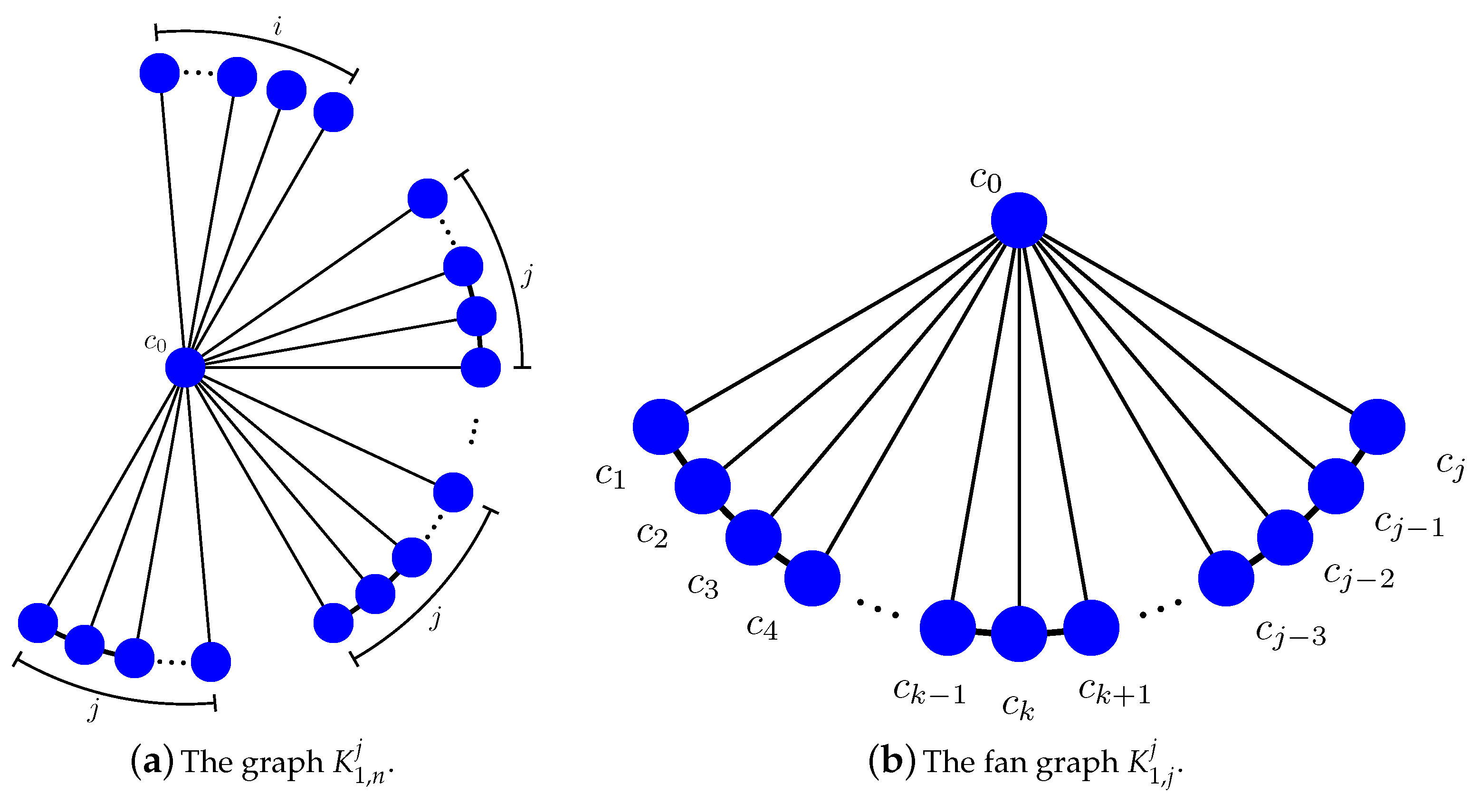
Let be a weighted star on vertices with center , vertex weight function for all , and edge weight function for all . Suppose the n leaves are labeled, in counterclockwise order, , then the wheel graph is obtained from by adding the edges for (here we let ).
As is well known, star
and wheel graphs
are very typical network topologies used in designing and implementing communication networks. The wheel graph
is the planar graph with a chromatic number not greater than 4. Specifically, the chromatic number of
is 3 for odd
n and 4 for even
n. Some researchers have tried to apply this property of
to prove the famous Four Color Theorem [
36]. Moreover,
can also be used in wireless ad hoc networks [
37]. Therefore, it is worth studying the new structural characteristics of these two graphs, especially from new perspectives.
Inspired by the significant effect of graph surgeries on evolutionary dynamics in [
38], we are motivated to study the subtree number in graphs resulting from graph surgeries. In particular, we will consider a class of graphs that “lie in between” the fan and wheel graphs, called the “partitions” (explanation will be given later) of wheel graphs.
Definition 1. Given the star on vertices defined above with center vertex and , the graph is obtained from by adding the edges for all except for (see Figure 1a). If , we call the fan graph on vertices. It is also easy to see that is the single vertex , and is the star . From the definitions of the graph and the wheel graph , we see that the graph can be vividly described in terms of through “partitions” (and deletion of edges ) perspective.
The reason that we consider our graphs as vertex and edge weighted is to use the so-called subtree generating functions. We assume a graph to be a weighted graph and define the vertex-weight function and edge-weight function , where ℜ is the real number. Unless otherwise noted, for a graph G, we initialize its vertex weight function for each and its edge weight function for each throughout this paper.
The following notations need to be listed before introducing the main tool:
denotes the graph obtained from G by removing all elements of X;
(resp. ) denotes the set of subtrees of G (resp. containing v);
denotes the set of subtrees of G containing the edge ;
denotes the weight of subtree ;
is the sum of weights of subtrees in ;
is the cardinality (namely the number) of the corresponding set of subtrees.
We define the weight of a subtree of G, denoted by , as the product of the weights of the vertices and edges in . The generating function of subtrees of G, denoted by , is the sum of weights of subtrees of G. Namely, . Similarly, we define
By substituting each vertex weight and edge weight in these generating functions, we have the corresponding numbers of subtrees under various constraints, i.e., and .
We introduce the following lemma, which will frequently be used in our work.
Lemma 1. [4] Let be a path on n vertices, with vertex weight function for all and edge weight function for all , then . In
Section 2, we will present the subtree generating functions of
and the wheel graph
. Through using these generating functions and theoretical analysis, we study the extremal graphs, subtree fitting problems, and subtree density behaviors of these graphs in
Section 3. Lastly, in
Section 4, we summarize our results and comment on potential topics for future work.
2. Subtree Generating Functions of and Wheel Graph
In this section, we will establish the subtree generating functions of and wheel graph and provide the theoretical background for our computational analysis. We start by studying the subtree problem of .
2.1. Subtree Generating Functions and Subtree Numbers of
Theorem 1. Let be the weighted graph defined as above, and be non-negative integers with and . Thenwith , and , . Proof. We consider the subtrees of by cases
- (i)
not containing the center ,
- (ii)
containing the center .
From Lemma 1, we have the subtree generating function of case (i) as
With the contraction method of [
4] and structure analysis, we have the subtree generating function of case (ii) as
Denote
and
, and divide all subtrees for
(see
Figure 1b) into four cases
where
is the collection of subtrees that contain neither nor ;
is the collection of subtrees that contain , but not ;
is the collection of subtrees that contain , but not ;
is the collection of subtrees that contain both and .
From the definitions of subtree weight and subtree generating function, we know that:
(a) ;
(b) , where are the trees obtained from by attaching an edge at vertex ;
(c) We can write
as
for
and
;
(d) For each subtree , we know that must not contain the edge . Consequently, we can further consider the subtrees that contain edges but not recursively for .
Hence, by Equations (
5)–(
8), we have
with
,
.
Combining Equations (
2), (
3), and (
9), we have Equation (
1) and the theorem follows. □
Following similar arguments to Theorem 1, we can also obtain the subtree generating functions of the graphs obtained from identifying the centers of different fan graphs (). We skip the tedious details for the sake of space.
Theorem 2. Let be different weighted fan graphs, and suppose there are copies of for . Let be the graph that is constructed by identifying the centers of these fan graphs with . Thenwith and , . Actually, a single fan graph is a special case of the above discussion, so we can further obtain the subtree generating function for the subtrees containing a particular vertex. Again, we skip the similar but technical details.
Theorem 3. Let be a weighted fan graph with vertex weigh f and edge weigh g (see Figure 1b), thenwith and , . Adding an edge between any two fan graphs (to construct a bigger fan) of a graph will also increase the number of subtrees. Let G be the weighted graph as defined in Theorem 2, and suppose (with non-center vertices labeled counterclockwise as ) and (with non-center vertices labelled clockwise as ) are the two sub-fan graphs of G with . Define to be the graph obtained from G by adding one edge . Meanwhile, denote the graph of that contains , and denote the collection of subtrees in that contain . By dividing the subtrees of G and into two cases of containing center or not, with Lemma 1, definitions of subtree weight and subtree generating function, and combining structure analysis, we have the following theorem:
Theorem 4. Let G and be the weighted graphs defined above. Then, By letting in the subtree generating functions from the above theorems, we have the corresponding subtree numbers of the various related graphs above.
Corollary 1. The subtree number of iswith . With Corollary 1, we have the number of subtrees of
that contain central vertex
as illustrated in
Figure 2.
Corollary 2. Let be positive integers with , and , thenwith and . With Corollary 2, we have the subtree number of
, see details in
Section 3.1.
Corollary 3. Let , , and l be defined in Theorem 2, thenwith and , . Let be the graph defined in Theorem 2 with ; ; ; , with Corollary 1 and Corollary 3, we have .
Corollary 4. The number of subtrees of the fan graph containing iswith and , . Similarly, the number of subtrees of
that contain central vertex
(see
Figure 3) can be obtained from Corollary 4.
Corollary 5. Let G be the graph defined in Theorem 2, and be a merged graph from G with and (Theorem 4), thenwhere is the number of subtrees containing both vertex and edge . Let G, , and be the graphs defined in Corollary 5 with ; , and , with Corollary 1, Corollary 5, and structural analysis, we have = 77,997, , and = 129,303.
2.2. Subtree Generating Function and Subtree Number of Wheel Graph
Next we consider the subtree generating function of the weighted wheel graph .
Theorem 5. Let be the weighted wheel graph on vertices with vertex weight function and edge weight function . Thenwith , , , and . Proof. For convenience, we let for , and for . We also follow the convention that if , and , if .
We first consider the subtrees of in different cases:
(i) not containing the edge ,
(ii) containing the edge .
The subtrees in case (i) can be further partitioned into four categories. As a result, we have
where
is the set of subtrees of that contain neither nor ;
is the set of subtrees of that contain , but not ;
is the set of subtrees of that contain but not ;
is the set of subtrees of that contain both and .
From the definition of subtree weight and with structure analysis, we have
and
Similarly, for case (ii), we have
where
is the set of subtrees in that contain neither nor ;
is the set of subtrees in that contain , but not ;
is the set of subtrees in that contain but not ;
is the set of subtrees in that contain both and .
Analyzing each case, we have:
(a) , where are the trees obtained from by attaching the edge at vertex ;
(b) , where is the graph of that contains , and obviously, ;
(c) for ;
(d) In a similar manner as (b) and (c), use variables l and r to count the number of edges trailing off
and
, respectively, then the subtrees in
are indexed by these two variables, which count extra edges that are on the two sides of the T shape containing the 3 edges required by
. With (a)–(d), we have
Now with Equations (
23)–(
25), we have
By Theorem 1, Theorem 3, and Equations (
22) and (
26), we have
Note that
is not a wheel graph. With Theorem 1 and Lemma 1, we have
Now from Equations (
27) and (
28), we have
The subtree generating function of
now follows from Equations (
27) and (
29). □
Letting
in Equation (
18), we have the following corollary.
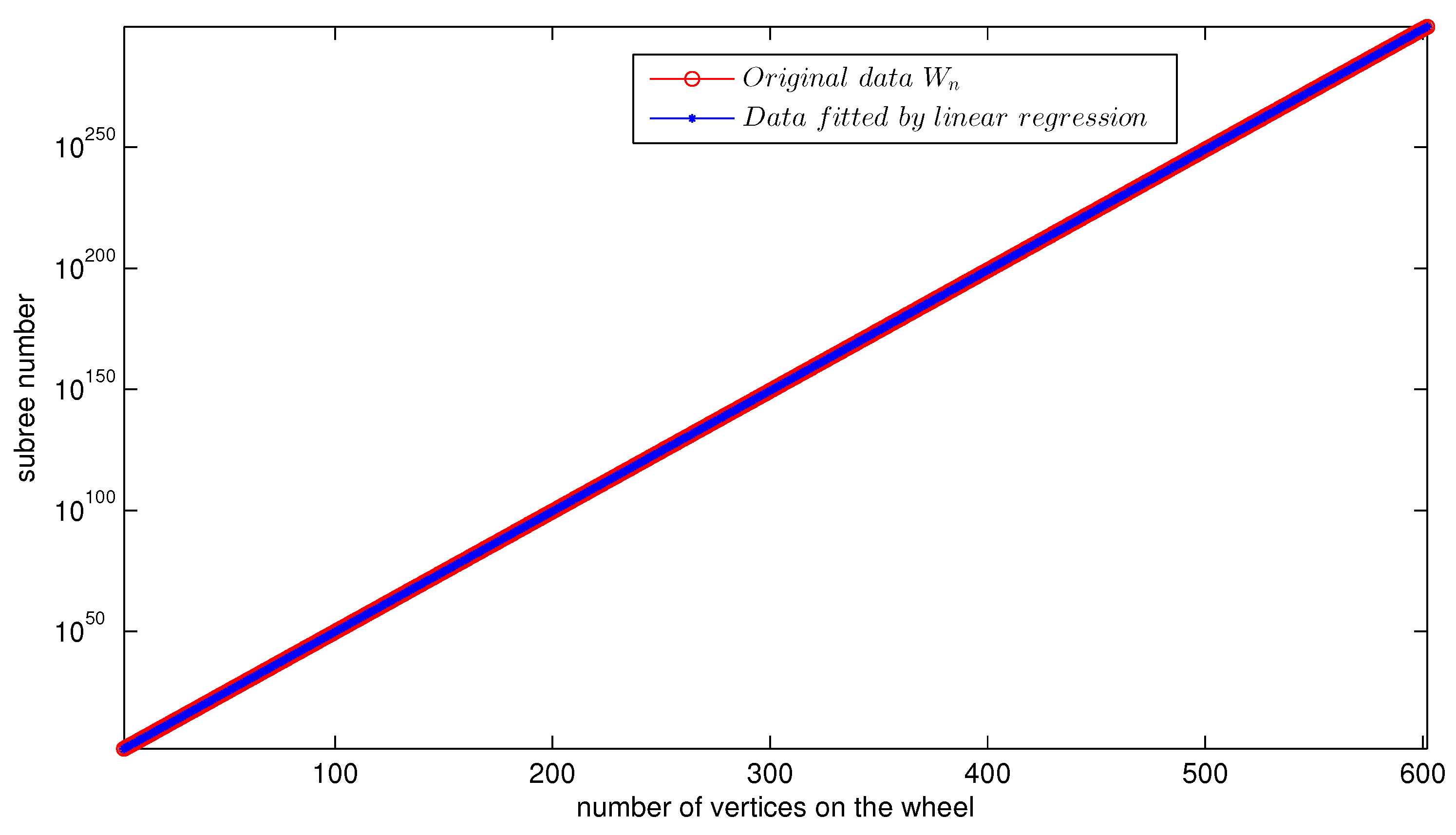
Corollary 6. The subtree number of iswith , , and . With Corollary 6, the subtree numbers of
are shown in
Table 1.
As a matter of fact, with the generating function and further structural and theoretical analysis, we can also solve the subtree generation computing problems for the following more generalized types of graphs; here we skip the similar but technical details.
(i) Graph is constructed by identifying the center of l graphs to , where is the graph constructed from a vertex and a path by connecting with , , and any other arbitrary vertices on the path ; for the special case , the graph is a path on vertices and .
(ii) Graph , namely the graph obtained from wheel by deleting random l different edges (each is different the others).


