1. Introduction
With the rapid development of technology in recent years, the engineering system has become increasingly complex. The growing complexity of the system provides a new source of uncertainty. Uncertainty arises because some design parameters may be changed over the course of development, or they cannot yet exactly be specified [
1,
2,
3]. The uncertainty appears as a deviation between the desired and realized parameter settings, which may bring in design failure, therefore it is essential to improve design under the uncertainty for complex systems.
Design points that achieve their design goals are called good, otherwise they are called bad. However, if there is already a bad design point, engineers are interested in how to turn it into a good design with the least effort. It can be fulfilled by modifying as few parameters from the existing bad design as possible.
Traditional optimization [
4], sensitivity analysis [
5,
6], robust design optimization [
7,
8,
9], and reliability-based design optimization [
10,
11,
12] are some classical approaches to improve designs. Traditional optimization seeks an optimum design point in the design space, which does not take uncertainty into account. Sensitivity analysis computes the effect of variability of input design parameters on variability of output performance value. Unfortunately, sensitivity analysis does not provide information on how the parameters of a bad design need to be changed in order to turn it into a good design. Robust design optimization seeks a design point in a deterministic neighborhood with small output variation. However, robust design optimization only deals with the case where the variability of design parameters is given. If the variability of the design parameters is not completely known, it has to be estimated, which is not always possible. Reliability-based design optimization is a method to determine optimal designs which are characterized by a low probability of failure. Unfortunately, it is established under the assumption that the complete information of the design uncertainty is known.
Evolutionary algorithms are often used to solve design optimization problems in the presence of uncertainties [
13,
14,
15,
16]. The non-dominated sorting genetic algorithm II is combined with reliability-based optimization for handling uncertainty in design parameters in [
13]. Six-sigma robust design optimization is solved by the many-objective decomposition-based evolutionary algorithm in [
14]. Evolutionary algorithms have some specific advantages, which include the ability to self-adapt the search for optimum solutions on the fly, as well as the flexibility of the procedures.
Besides, swarm intelligence-based algorithms are frequently-used techniques in design optimization problems [
17,
18,
19,
20]. The uncertainty is directly incorporated into optimization using particle swarm, and a deterministic Pareto front of optimal designs is found in [
17]. The ant colony optimization is combined with reliability-based design optimization to achieve the global optimal design of a crane metallic structure under parametric uncertainty in [
18]. Against the uncertainty of cost and traffic, a mathematical model is established using robust optimization method, and the corresponding optimal design is obtained by ant colony algorithm in [
19]. Swarm intelligence-based algorithms often find an optimal solution when appropriate parameters are determined and sufficient convergence stage is achieved.
The solution hyper-box on which all design points are good is expressed by independent target intervals for each design parameter. The widths of target intervals quantify the robustness to uncertainty. Furthermore, the solution hyper-box can help to improve a bad design. More precisely, a bad design can be turned into a good one by only moving its design parameters into their target intervals. To make it easy to reach the target intervals, the solution hyper-box should be as large as possible.
There are two categories of approaches which seek for a solution hyper-box with the maximum volume in the literature. The first category is based on machine learning and data mining techniques [
21,
22,
23]. A stochastic method is presented in [
21], which combines online learning and query. It probes a candidate solution hyper-box by stochastic sampling, and then readjusts its boundaries in order to remove bad designs and explores more design space that has not been probed before. Because the locations of good and bad designs are estimated by Monte Carlo sampling, the obtained solution hyper-box may not have the maximum size. The second category is based on an analytical technique [
24,
25,
26]. The algorithm presented in [
24] applies interval arithmetic within an iterative optimization scheme to check whether the candidate hyper-box is a solution hyper-box. However, interval arithmetic limits the applicability of the algorithm, as the accuracy of the interval arithmetic depends on the problem. Besides, the interval arithmetic cannot handle the black-box performance function. The algorithm proposed in [
26] combines the DIRECT algorithm [
27] with evolutionary algorithms, where the former is a checking technique to guarantee that the obtained hyper-box is indeed a solution hyper-box and the latter is to seek the maximum size of hyper-box. Unfortunately, the DIRECT algorithm requires very high computational effort for its work.
This paper aims to turn a bad design into a good one with comparatively little effort in the presence of uncertainty. To this end, instead of focusing on an optimal design point, an approach based on the optimization of the solution hyper-box is proposed in this paper. Specifically, design parameters are classified into key parameters and non-key ones based on engineering knowledge firstly. Secondly, by adding proper constraints on non-key parameters, we seek the maximum solution hyper-box which already includes non-key parameters of the bad design. The maximum solution hyper-box provides the target intervals for each design parameter. Finally, the bad design is turned into a good one by only moving its key parameters to their target intervals. Obviously, the wider the target interval is, the stronger the robustness is against unintended variations.
Therefore, we focus on seeking for the maximum solution hyper-box which is in compliance with constraints. Fender et al. [
28] extended the algorithm in [
21] to account for constraints. However, the algorithm in [
28] produces a hyper-box that may not have the largest size and may contain some bad designs, because the locations of good and bad designs are estimated by the Monte Carlo sampling. In this paper, the proposed PSO-Divide-Best method combines particle swarm optimization (PSO) [
29] with the Divide-the-Best algorithm in [
30], where the former is to evolve the solution hyper-box towards larger volume and the latter is to guarantee that the obtained solution hyper-box only includes good designs. The PSO-Divide-Best method is established based on black-box performance functions, so it is appropriate for most engineering problems.
The paper is organized as follows. The next section explains the motivation of this paper and gives a mathematical problem statement for optimizing the solution hyper-box with constraints.
Section 3 introduces the Divide-the-Best algorithm and particle swarm optimization.
Section 4 presents the proposed approach in detail. In
Section 5, we apply the proposed approach to complex systems. In
Section 6, we provide some concluding remarks.
4. The Proposed Particle Swarm Optimization Divide-the-Best Algorithm
The particle swarm optimization algorithm does not rely on mathematical properties for application. The Divide-the-Best algorithm in [
30] is an efficient algorithm to calculate the global minimum of a black-box performance function over a hyper-box. Therefore, an innovative approach which combines the particle swarm optimization algorithm with the Divide-the-Best algorithm is proposed to solve the problem (
7), referred to as the particle swarm optimization divide-the-best algorithm (PSO-Divide-Best).
Specifically, particle swarm optimization drives the evolution toward increasing the volume of hyper-box. The Divide-the-Best algorithm solves the optimization sub-problem (
8), and thus ensures that the obtained hyper-box only includes good designs.
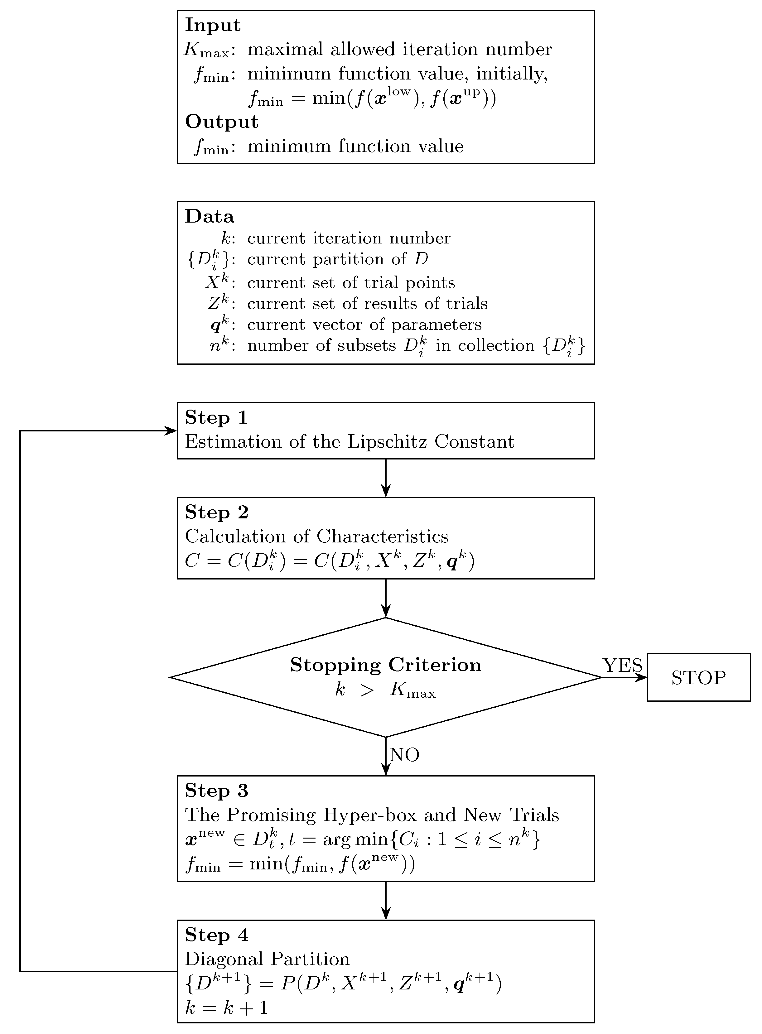
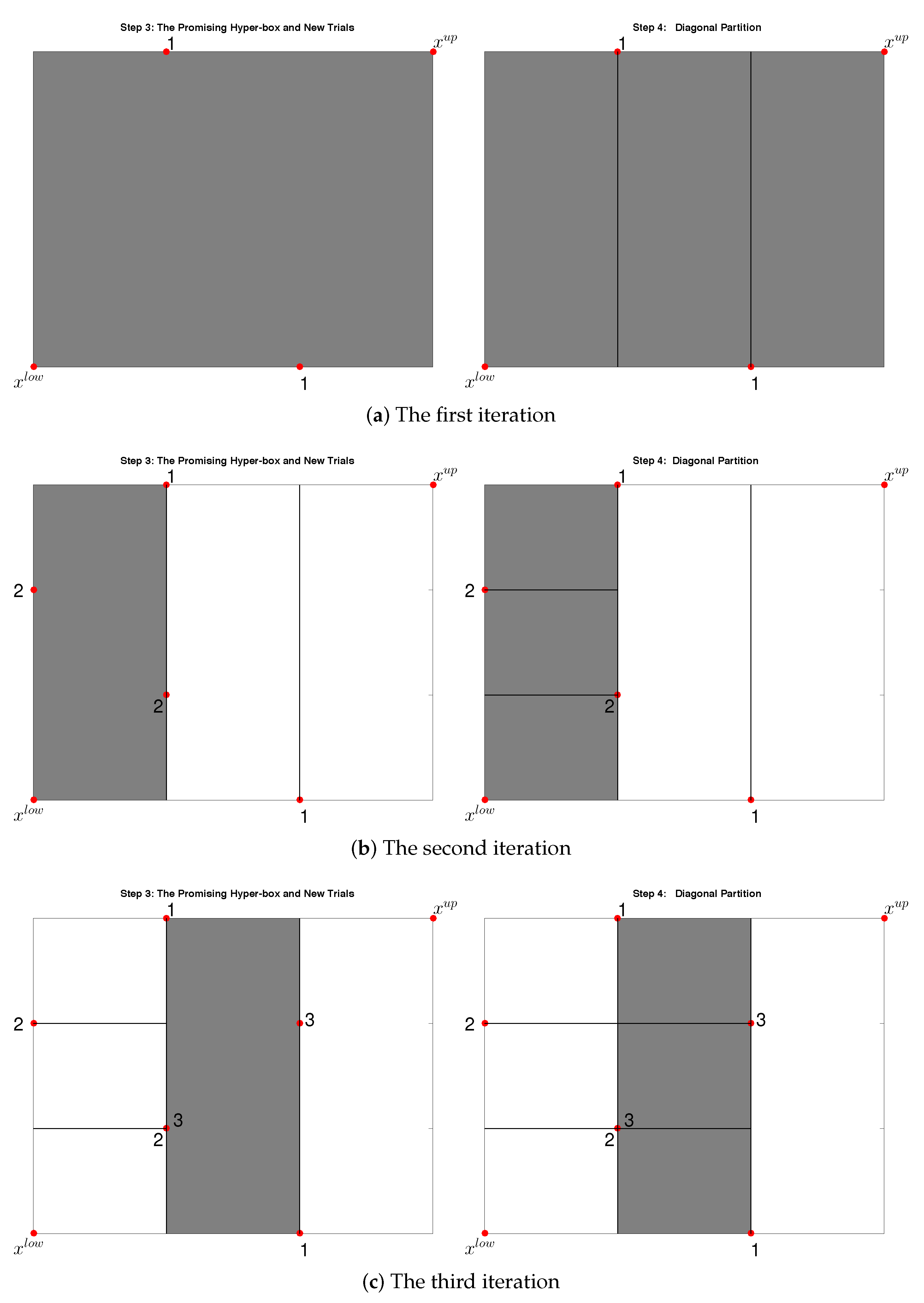
The PSO-Divide-Best algorithm is illustrated in Algorithm 1. Initially, it generates randomly a group of particles satisfying constraints. During the process of optimization, at iteration
t, firstly, the velocity
and position
of the
ith particle are updated according to Equations (
9) and (
10), respectively. Then, if the conditions
,
, and
are not satisfied, the re-updating is performed. Otherwise, the value of
is evaluated by the Divide-the-Best algorithm in
Figure 3 and denoted by
. If the constraint
is met, we calculate the corresponding volume according to Equation (
6), otherwise the particle is re-updated. Next,
and
are updated.
| Algorithm 1 The particle swarm optimization divide-the-best algorithm (PSO-Divide-Best) |
- Input:
The allowed maximum iteration number, ; The weight factors, and ; The initial and final weight parameters, and ; The number of particles, N; The current iteration number, ; - Output:
The lower and upper bounds of the maximum solution hyper-box, and ;
- 1:
Initialization: Initialize N particles randomly while satisfying constraints. - 2:
Optimization:
- 2.1
Velocity and position updates while satisfying constraints: for all do - 2.1.1
The ith particle velocity is updated according to Equation ( 9). If a particle violates the velocity limits, set its velocity equal to the limit. - 2.1.2
The position of each particle is modified by Equation ( 10). If a particle violates its position limits in any dimension, set its position equal to the limit. - 2.1.3
Set , , ; Set , . - 2.1.4
If the constraints , , , are not satisfied, go to Step 2.1.1. - 2.1.5
Calculate the value of by algorithm in Figure 3 with parameter setting , denoted by . - 2.1.6
If the constraint is met, then calculate the corresponding volume by Equation ( 6), namely . Otherwise go to Step 2.1.1.
end for - 2.2
Update and :
- 2.2.1
For all , if , set and . - 2.2.2
Update as the one with the maximum volume among all , .
- 2.3
Stopping criteria: If , set and go to Step 2.1.
- 3:
Verification:
- 3.1
Set , , ; Set
, . - 3.2
Calculate the value of by algorithm in Figure 3 with parameter setting , denoted by . - 3.3
If , output and ; Otherwise go to Step 2.
|
Finally, to verify whether the best particle satisfies the constraints, the Divide-the-Best algorithm with more iterative times is performed. If the constraints are satisfied, PSO-Divide-Best outputs the best particle. Otherwise, it goes back to Step 2.
PSO is derivative-free and global search [
43]. The Divide-the-Best algorithm in [
30] can converge to the global minimum with any degree of accuracy provided there are enough iterations. Therefore, the proposed PSO-Divide-Best method in this paper has the following advantages:
- (1)
PSO-Divide-Best has great possibility to reach the globally maximum solution hyper-box satisfying the constraints.
- (2)
Due to the discrete nature of the trial points in the Divide-the-Best algorithm, the PSO-Divide-Best method can be applied to both analytically known and black-box performance functions.
- (3)
PSO-Divide-Best guarantees that any point selected within the obtained hyper-box is a good design provided that the performance function is continuous.
In most engineering problems, the performance function is continuous whether it is analytically known or black-box. Therefore, the PSO-Divide-Best approach has strong applicability in engineering problems.
5. Case Studies
A stochastic approach based on Monte Carlo sample is discussed in [
28]. This approach consists of two phases: exploration phase and consolidation phase. The purpose of the exploration phase is to identify a solution box as large as possible. The consolidation phase includes an algorithm which shrinks the hyper-box such that it contains only good designs. Therefore, we denote this method by “EPCP” hereafter (an abbreviation for “exploration phase and consolidation phase”). Besides, a method in [
24] which combines interval arithmetic with cellular evolutionary strategies is denoted by “IA-CES” hereafter.
To compare the proposed PSO-Divide-Best method with the EPCP and IA-CES ones, two cases are considered. The first case is the vehicle structure design problem which has been studied by Fender et al. in [
28]. The second case is the power-shift steering transmission control system (PSSTCS) with a price of approximately 500,000 USD.
In the proposed PSO-Divide-Best method, the weight factors and are set to 2, the maximum number of iterations is 2000, , , and the number of particles N is set to 160.
All experiments were performed in MATLAB R2016b on a windows platform with Intel Core i7-4790 CPU 3.60 GHz, 16 GB RAM.
5.1. Vehicle Structure Design Problem
The vehicle structure design problem in [
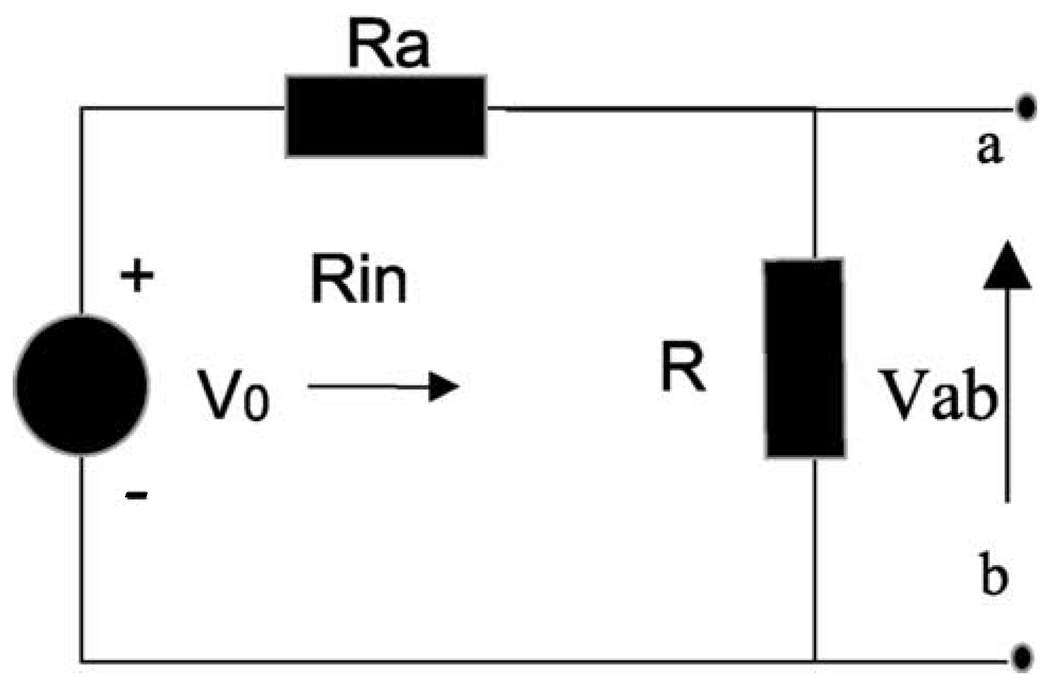
28] consists of two structural components. The design parameters are the two deformation forces
and
. The performance functions are as follows:
where
,
kg is the mass,
g is a critical threshold level,
m/s is the speed, and
m are the limits of the deformation measures. The design goals are achieved if
for all
.
A design with
kN and
kN is considered in [
28]. It violates Equation (
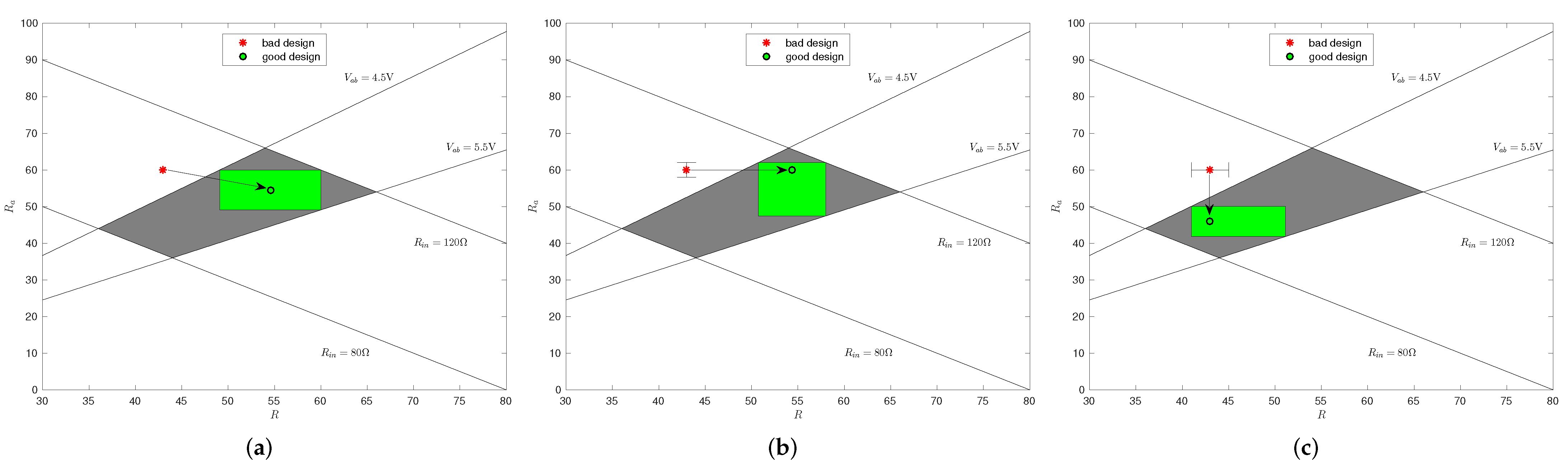
11a) and therefore is a bad design. To improve this bad design with the least effort, three scenarios are performed. In Scenario (a), both
and
are key parameters, that is, both
and
need to be modified. In Scenario (b), only
is the key parameter. More precisely,
is included in the solution hyper-box that is obtained by requiring a minimum safety margin of
. In Scenario (c), only
is the key parameter.
Since each performance function in Equation (11) is monotone, the exact solution is obtained by the penalty method [
44], as shown in
Table 1. The results in [
28] obtained by the EPCP method are listed in
Table 1. Due to the stochastic nature of the PSO, as adopted in [
24], we ran the PSO-Divide-Best algorithm 20 times for each scenario, and the best solutions among the 20 runs are shown in
Table 1. The results obtained by the IA-CES method are also shown in
Table 1. The deviations between the lower boundaries computed numerically
and the exact solutions
are given by
. The relative error is given by
. Besides, the relative error for the upper boundaries of the hyper-box are defined in a similar way. The row entitled “volume” is the volume of hyper-box, and the row entitled “error” is the relative error between the volume of hyper-box computed numerically and the exact one.
Table 1 shows that the hyper-boxes obtained by the PSO-Divide-Best method are nearly identical to the exact ones, while the hyper-boxes obtained by the EPCP and IA-CES approaches have a high deviation from the exact ones. Besides, the hyper-boxes obtained by the PSO-Divide-Best method are significantly larger than those obtained by the EPCP and IA-CES methods.
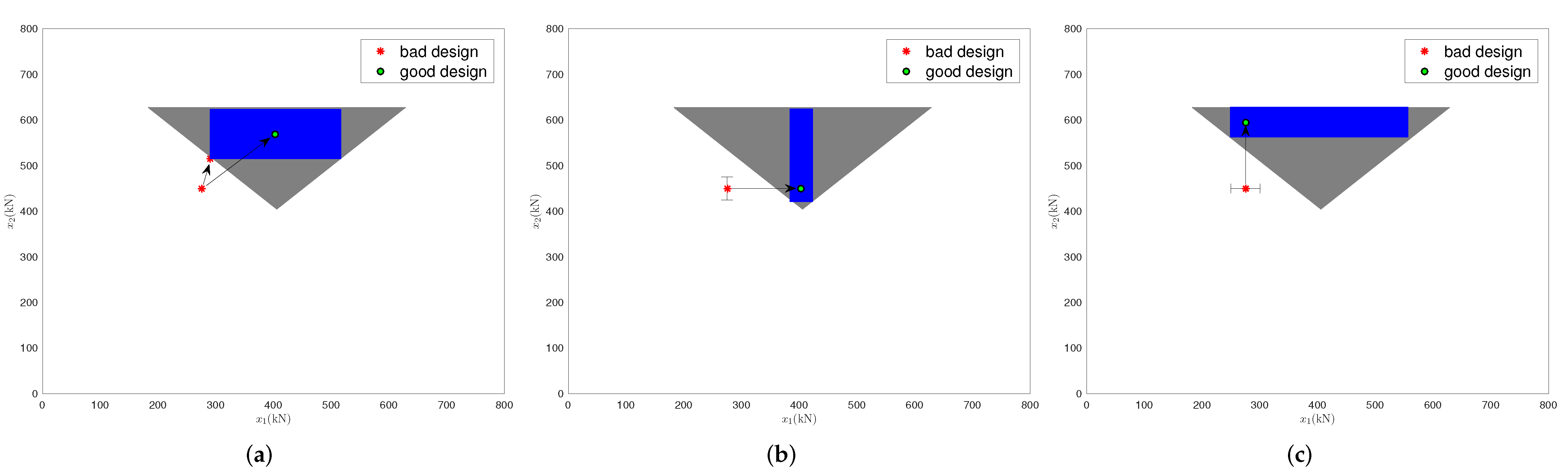
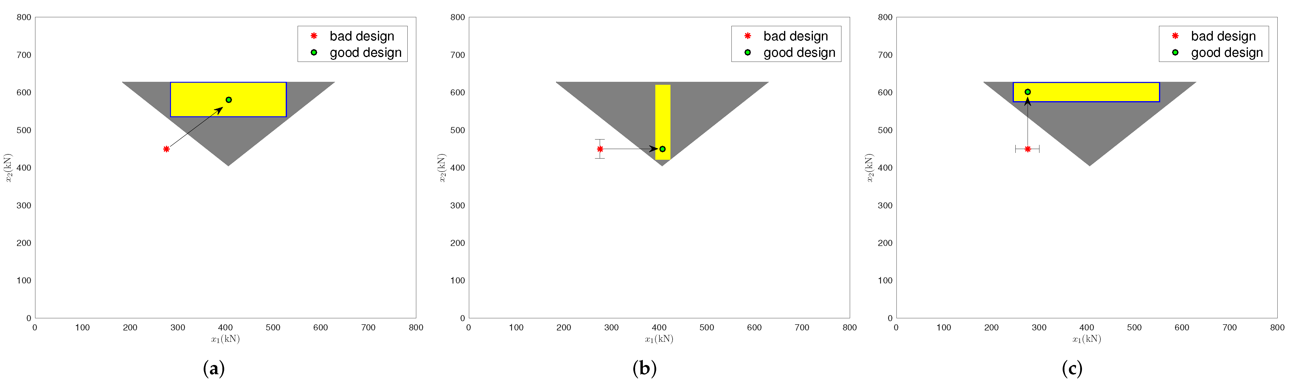
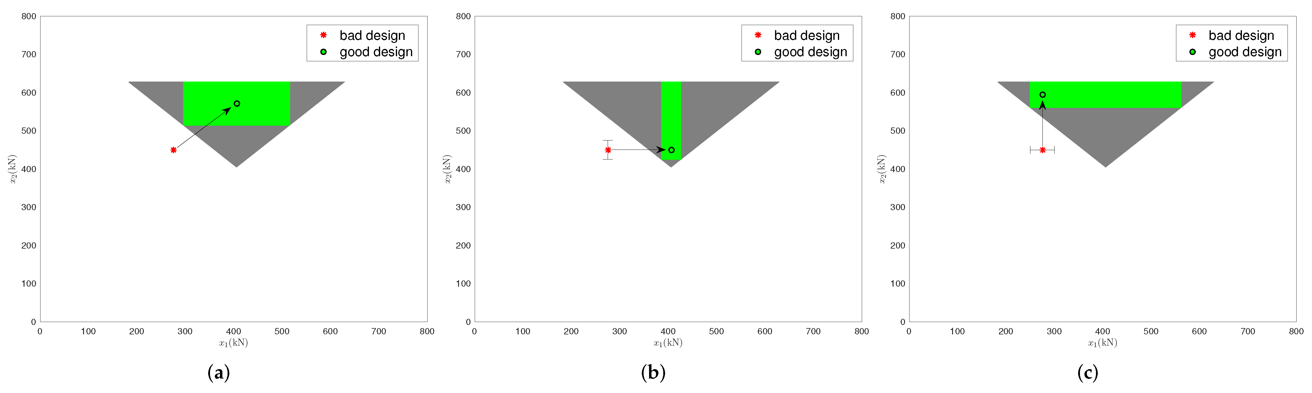
Furthermore, a visualization of the results of the EPCP, IA-CES, and PSO-Divide-Best methods in
Table 1 is shown in
Figure 5,
Figure 6 and
Figure 7, respectively, where the grey region is the complete solution space.
Figure 5,
Figure 6 and
Figure 7 also give some examples of how to turn the bad design into a good one.
In Scenarios (a) and (b), the blue hyper-boxes exceed the grey region. This implies that the hyper-boxes obtained by the EPCP method contain some bad designs. Based on the hyper-box obtained by the EPCP method, a bad design may fail to be turned into a good one (see
Figure 5a). Consequently, the EPCP method should be used with great caution.
The yellow hyper-boxes obtained by the IA-CES method all lie within the grey region; however, they are not the largest ones. This implies that target intervals for each parameter determined by the IA-CES method are relatively shorter. Therefore, the good design point which is determined by the IA-CES method has relatively poor robustness against unintended variations.
The green hyper-boxes obtained by the PSO-Divide-Best method all locate within grey region, therefore they only include good designs. Actually, as long as the key parameters of the bad design are moved into their target intervals defined by our method, the bad design is turned into a good one. Taking Scenario (b) as an example, according to the solution hyper-box obtained by the PSO-Divide-Best method shown in
Table 1, the bad design is turned into a good one by changing
into any value within
.
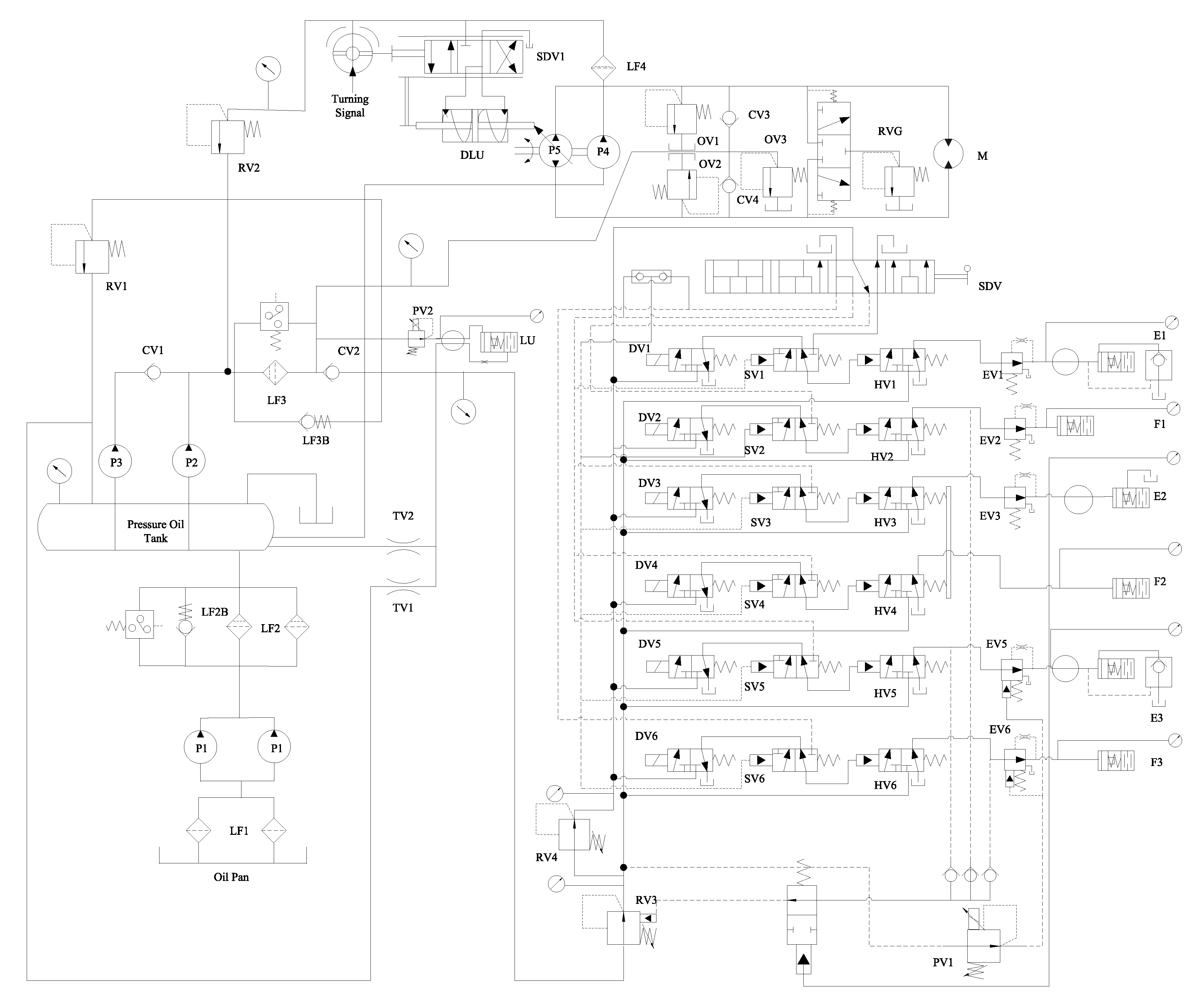
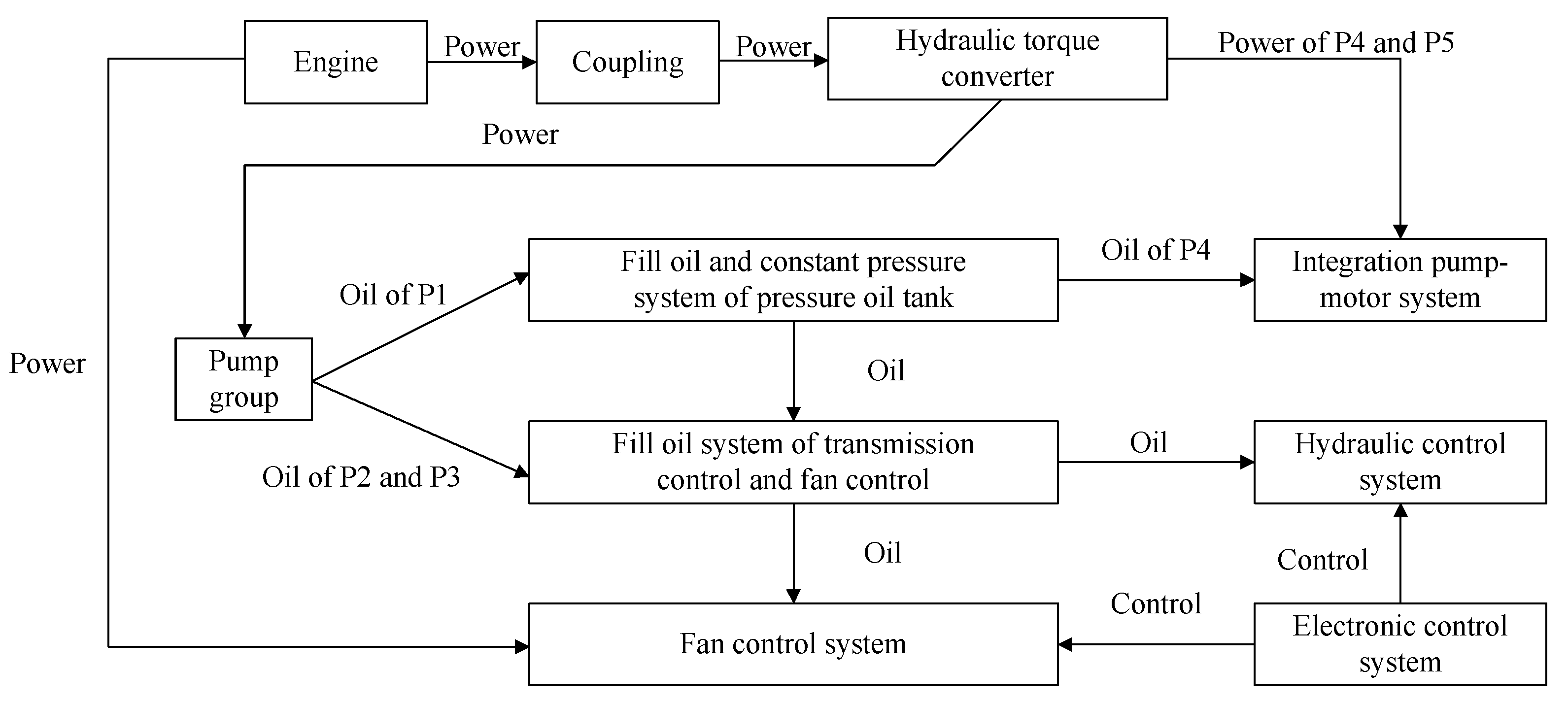
5.2. The Power-Shift Steering Transmission Control System (PSSTCS)
Figure 8 and
Figure 9 show the structure principle drawing and the function constitutes of PSSTCS, respectively.
The PSSTCS is a non-monotonic coherent system which consists of 86 components. The design goal is that the system reliability should be higher than 0.9900. However, the system reliability function is not analytically known, so it is evaluated by the goal-oriented (GO) reliability assessment method in [
45]. Now, we consider a design shown in
Table A1 in
Appendix A. Its system reliability is 0.9856; therefore, it is insufficient. To improve this bad design with the least effort, firstly, the engineers classify design parameters into key parameters and non-key ones according to modification difficulty degree. The key parameters (components) are marked with red color in
Table A1. Secondly, we search the maximum solution hyper-box which already includes non-key parameters of this bad design. More precisely, in this PSSTCS case, the optimization problem (
7) is formulated as follows:
where
,
,
and
are the lower and upper bounds of reliability for the
ith component,
,
is the reliability for the
ith component,
,
,
,
,
,
is the reliability threshold, and
is the system reliability function which is evaluated by the GO method in [
45]. Note that the volume here is replaced by the log-volume (logarithmic transformation of the volume) in order to calculate conveniently.
The IA-CES method is established based on analytically known function; therefore, it is not applicable to this complex system with black-box reliability function. The obtained hyper-boxes of the problem (
12) by the EPCP and PSO-Divide-Best methods are listed in
Table A2 in
Appendix A. We see that the lower bounds obtained by the PSO-Divide-Best method are almost always smaller than those obtained by the EPCP method, and the upper bounds obtained by the PSO-Divide-Best method are almost always larger than those obtained by the EPCP method. This implies that the PSO-Divide-Best method provides much wider target intervals for most design parameters. Therefore, the PSO-Divide-Best method has stronger robustness against uncertainty.
Besides, the log-volume of the obtained hyper-box is listed in
Table 2. We see that the log-volume of hyper-box obtained by the PSO-Divide-Best method is much larger than that by the EPCP method. This is further reflected that the PSO-Divide-Best method is more robust against variations.
The hyper-box provides target intervals for each design parameter; therefore, the bad design can be turned into a good design by only moving its key parameters into their target intervals. Particularly, the good design for which the key parameters are located at the midpoints of their target intervals may be the most representative one. It provides the maximum robustness if the variation of design parameter is the same on both sides of a nominal value. These representative good designs obtained by the EPCP and PSO-Divide-Best methods are listed in
Table A1. To verify whether these good designs satisfy the design goal, their system reliabilities were evaluated by the GO method, as also shown in
Table A1. We can see these two good designs indeed achieve the design goal. Therefore, the system reliability for the PSSTCS can change from insufficient to sufficient by only modifying the reliabilities for key components according to
Table A1.
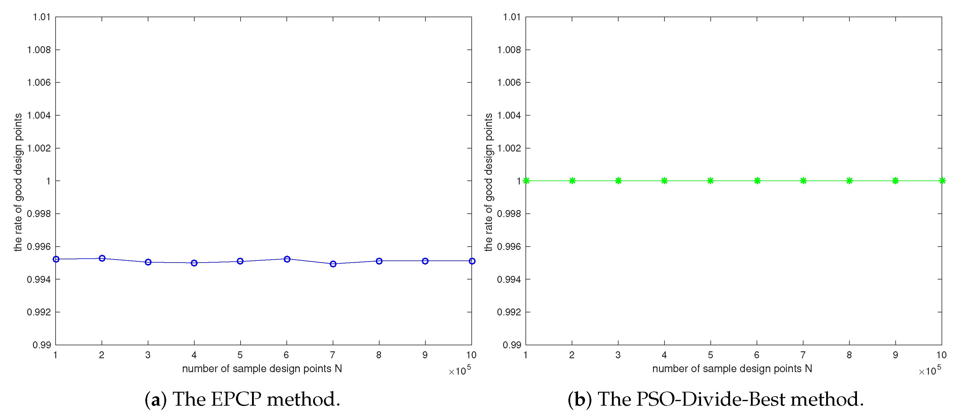
To illustrate whether the obtained hyper-boxes meet the design goal, we use the Latin hypercube sampling to choose
n designs from each hyper-box, and then calculate the rate of good designs as follows:
where
is the indicator function, i.e.,
if
and
otherwise.
Figure 10 shows the rates of good designs under different sample sizes. We see that the rates of good designs of the PSO-Divide-Best method are all 1, while those of the EPCP method are all below 1. This implies that the hyper-box obtained by the PSO-Divide-Best method only includes good designs, while those obtained by the EPCP method includes some bad designs. Therefore, the EPCP method should be used cautiously, because it may fail to turn a bad design into a good one. However, the PSO-Divide-Best method is valid as it ensures any design within the obtained hyper-box is good.
6. Conclusions
To improve a bad design with comparatively little effort in the presence of uncertainty, rather than changing all design parameters of this bad design, this paper only modifies its key parameters. To this end, the maximum solution hyper-box which already includes non-key parameters of a current bad design is sought. The solution hyper-box provides target intervals for each design parameter. A current bad design can be turned into a good one by only moving its key parameters into their target intervals. The volume of the solution hyper-box should be as large as possible for providing stronger robustness against unintended variations.
The PSO-Divide-Best algorithm combines the PSO and the Divide-the-Best algorithms [
30] to seek a solution hyper-box which has the maximum volume and satisfies all the constraints. The case studies show the solution hyper-boxes obtained by the PSO-Divide-Best method only include good designs, and they are much larger than those obtained by the EPCP and IA-CES methods. This implies that a good design determined by the EPCP method may have stronger robustness against uncertainty. Therefore, our method is better than the EPCP and IA-CES methods.
Since the Divide-the-Best algorithm only evaluates the performance function at trial points, the PSO-Divide-Best method has strong application and can be applied to complex systems with black-box performance functions. As long as the performance function is continuous, our method can provide a solution hyper-box that is guaranteed to include only good designs. Therefore, a bad design can be turned into a good one provided that its key parameters are moved into the target intervals obtained by our method. This implies that our method is valid. Our method converges to the globally maximum solution hyper-box with very great probability. However, its convergence speed becomes slow as the number of design parameters increases. Therefore, the scalability of our method is relatively poor.


