1. Introduction
In the field of bioinformatics, strings are commonly used to model sequences such as DNA, RNA, and protein molecules or even time series. Strings represent fundamental data structures in many programming languages. Formally, a string
s is a finite sequence of
letters over (usually) a finite alphabet
. A subsequence of a string
s is any sequence obtained by removing arbitrary letters from
s. Similarities among several strings can be determined by considering common subsequences, which may serve for deriving relationships and possibly to distill different aspects of the of input strings, such as mutations. More specifically, one such measure of similarity can be defined as follows. Given a set of
m input strings
, the
longest common subsequence (LCS) problem [
1] aims at finding a subsequence of maximum length that is common for all strings from the set of input strings
S. The length of the LCS for two or more input strings is a widely used measure in computational biology [
2], file plagiarism check, data compression [
3,
4], text editing [
5], detecting road intersections from GPS traces [
6], file comparison (e.g., in the
Unix command
) [
7] and revision control systems such as
Git. For a fixed
m, polynomial algorithms based on dynamic programming (DP) are known [
8] in the literature. These dynamic programming approaches run in
time, where
n denotes the length of the longest input string. Unfortunately, these approaches quickly become impractical when
m and
n get large. For an arbitrary large number of input strings, the LCS problem is
-hard [
1]. In practice, heuristic techniques are typically used for larger
m and
n. Constructive heuristics, such as the Expansion algorithm and the Best-Next heuristic [
9,
10], appeared first in the literature to tackle the LCS problem. Significantly better solutions are obtained by more advanced metaheuristic approaches. Most of these are based on
Beam Search (BS), see for example, [
11,
12,
13,
14,
15]. These approaches differ in various important aspects, which include the heuristic guidance, the branching scheme and the filtering mechanisms.
Djukanovic et al. (2019), in [
16], proposed a generalized BS framework for the LCS problem with the purpose of unifying all previous BS-based approaches from the literature. By respective parametrization, each of the previously introduced BS-based approaches from the literature could be expressed, which also enabled a more direct comparison of all of them. Moreover, a heuristic guidance that approximates the expected length of an LCS on uniform random strings was proposed. This way, a new state-of-the-art BS variant that leads on most of the existing random and quasi-random benchmark instances from the literature was obtained.
Concerning exact approaches for the LCS problem, an integer linear programming model was considered in [
17]. It turned out not to be competitive enough as it was not applicable to most of the commonly used benchmark instances from the literature. This was primarily due to the model size—too many binary variables and a huge number of constraints are needed even for small-sized problem instances. Dynamic programming approaches also quickly run out of memory for small-to-middle sized benchmark instances or typically return only weak solutions, if any. Chen et al. (2016) [
18] proposed a parallel
FAST_LCS search algorithm that mitigated some of the runtime weaknesses. Wang et al. (2011) in [
14] proposed another parallel algorithm called
QUICK-DP, which is based on the dominant point approach and employs a quick divide-and-conquer technique to compute the dominant points. One more parallel and space efficient algorithm based on a graph model, called the
Leveled-DAG, was introduced by Peng and Wang (2017) [
19]. Li et al. (2016) in [
20] suggested the
TOP_MLCS algorithm, which is based on a directed acyclic layered-graph model (called the irredundant common subsequence graph) and parallel topological sorting strategies used to filter out paths representing suboptimal solutions. A more enhanced version of the latter approach that utilizes Branch-and-Bound is proposed by Wang et al. (2021) in [
21]. An approximate algorithm based on the topological sorting strategy was developed and applied to COVID-19 data by Li et al. (2020) in [
22]. A specific Path Recorder Directed Acyclic Graph (PRDAG) model was designed and used for developing the Path Recorder Algorithm (PRA) by Wei et al. (2020) in [
23]. Recently, Djukanovic et al. (2020) in [
24] proposed an
search that is able to outperform
TOP_MLCS and previous exact approaches in terms of memory usage and the number of instances solved to optimality. Nevertheless, the applicability of this exact
search approach is still limited to small-sized instances. The same holds for the other exact techniques from the literature. In [
24], the
search also served as a basis for a hybrid anytime algorithm, which can be stopped at almost any time and can then be expected to yield a reasonable heuristic solution. In this approach, classical
search iterations are intertwined with iterations of
Anytime column search [
25]. This hybrid was able to outperform some other state-of-the-art anytime algorithms from the literature, such as PRO_MLCS [
26] and
Anytime Pack Search [
27], in terms of solution quality. To the best of our knowledge, this hybrid approach is still the leading method for the LCS problem on a wide range of benchmark sets from the literature.
The methods so-far proposed in the literature were primarily tested on independent random and quasi-random strings, where the number or occurrences of letters in each string is similar for each letter. In fact, we are aware of just one benchmark set with different distributions (
BB, see
Section 4), where the input strings are constructed in such a way so that they exhibit high similarity, but still the letters’ frequencies are similar. In practical applications, this assumption of uniform or close-to-uniform distribution of letters does not need to hold. Some letters may occur substantially more frequently than others. For example, if we are concerned with finding motifs in sentences of any spoken language, each letter has its characteristic frequency [
28]. Text in natural languages can be modeled by a multinomial distribution over the letters. The required level of model adaptation can vary depending on the distribution assumptions such as letter dependence of a particular language. Letter frequencies in a language can also differ depending on text types (e.g., poetry, fiction, scientific documents, business documents). For example, it is interesting that the letter ‘E’ is the most frequent letter in both English (12.702%) [
28] and German (17.40%) [
29], but only the second most common letter in Russian [
30]. Moreover, the letter ‘N’ is very frequent in German (9.78%), but not so common in English (6.749%) and Russian (6.8%). Motivated by this consideration, we develop a new BS-based algorithm exhibiting an improved performance for instances with different string distributions.
Unlike the BS proposed by Djukanovic et al. (2019) in [
16], our BS variant applies a novel guidance heuristic at its core as a replacement of the so far leading approximate expected length calculation. In addition to an improved performance in the context of non-uniform instances, the novel heuristic is easier to implement than the approximate expected length calculation (which required a Taylor series expansion and an efficiently implemented divide-and-conquer approach) and there are no issues with numerical stability. Our new BS version is time restricted in the sense that its running time approximately fits a desired target time limit. Moreover, it obtains high-quality results without the need for extensive parameters tuning.
The main contributions of this article can be summarized as follows:
We propose a novel search guidance for a BS which performs competitively on the standard LCS benchmark sets known from the literature and, in some cases, even produces new state-of-the-art results.
We introduce two new LCS benchmark sets based on multinomial distributions, whose main property is that letters occur with different frequencies. The proposed new BS variant excels in these instances in comparison with previous solution approaches.
A new time-restricted BS version is described. It automatically adapts the beam width over BS levels with regard to given time restrictions, such that the overall running time of BS approximately fits a desired target time limit. A tuning of the beam width to achieve comparable running times among different algorithms is hereby avoided.
In the following, we introducing some commonly used notation before giving an overview of the remainder of this article.
1.1. Preliminaries
By S, we always refer to the set of m input strings, that is, , . The length of a string s is denoted by , and its i-th letter, , is referred to by . Let n refer to the length of a longest string and to the length of a shortest string in S. A continuous subsequence (substring) of string s that starts with the letter at index i and ends with the letter at index j is denoted by ; if , this refers to the empty string . The number of occurrences of a letter in string s is denoted by . For a subset of the alphabet , the number of appearances of each letter from A in s is denoted by . For an m-dimensional integer vector and the set of strings S, we define the set of suffix-strings , which induces a respective LCS subproblem. For each letter , the position of the first occurrence of a in is denoted by , . Last but not least, if a string s is a subsequence of a given string r, we write .
1.2. Overview
This article is organized as follows:
Section 2 provides theoretical aspects concerning the calculation of the probability that a given string is a subsequence of a random string chosen from a multinomial distribution.
Section 3 describes the BS framework for solving the LCS problem, as well as the novel heuristic guidance. Moreover, the time-restricted BS variant is also proposed. In
Section 4, a comprehensive experimental study and comparison is conducted.
Section 5 extends the experiments by considering instances derived from a textual corpus. Finally,
Section 6 draws conclusions and outlines interesting future work.
2. Theoretical Aspects of Different String Distributions
Most papers in the literature are dedicated to the development and improvement of methods for finding an LCS of instances on strings that come from a uniform distribution. In our work, we propose new methods for the more general case, where strings are assumed to come from a multinomial distribution of strings. More precisely, for an alphabet , as a sample space for the letter of the strings, a multinomial distribution is determined by specifying a (real) number for each letter such that represents the probability of seeing letter and . Note that the uniform distribution is a special case of the multinomial distribution , with .
Assuming that the selection of each letter in a string is independent, each string can be considered a random vector composed of independent random variables, resulting in its probability distribution being completely determined by a given multinomial distribution. By a random string, in this paper, we refer to a string whose letters are chosen randomly in accordance with the given multinomial distribution.
Let r be a given string. We now aim to determine the probability that a random string s, chosen from the same multinomial distribution as string r, is a subsequence of the string r. We denote this probability by . In the next theorem, we propose a new recurrence relation to calculate this probability.
Theorem 1. Let r be a given string and s be a random string chosen from the same multinomial distribution. Then, Proof. It is clear from the definition of a subsequence that the empty string is a subsequence of every string and that a string cannot be a subsequence of a shorter one. Therefore, the cases
and
are trivial. In the remaining case (
),
follows from the law of total probability. □
The probability
in recurrence relation (
1) is dependent not only on the length of string
r, but also on the letter distribution of this string. Therefore, it is hard to come up with a closed-form expression for the general case of a multinomial distribution
. One way to deal with this problem is to consider some special cases of the multinomial distribution, for which closed-form expressions may be obtained.
2.1. Multinomial Distribution—Special Case 1: Uniform Distribution
The most frequently used form of the multinomial distribution considered in the literature is the uniform distribution. Since in this case, every letter has the same occurrence probability, probability
in the recurrence relation (
1) depends only on the lengths
and
and can be written more simply as
. This case is covered by Mousavi and Tabataba in [
12], where the recurrence relation (
1) is reduced as follows:
Probabilities
can be calculated using dynamic programming as described by Mousavi and Tabataba in [
12].
2.2. Multinomial Distribution—Special Case 2: Single Letter Exception
Let one letter
have occurrence probability
,
and each other letter
have occurrence probability
. For this multinomial distribution, recurrence relation (
1) reduces to:
where
Note that, besides lengths
and
, (
3) depends only on whether or not a letter in the string
r is equal to
.
2.3. Multinomial Distribution—Special Case 3: Two Sets of Letters
We now further generalize the previous case. Let
be a partitioning of the alphabet
, that is, let
be nonempty sets such that
and
. Let us assume that every letter in
has the same occurrence probability and also that every letter in
has the same occurrence probability. We define
where
is the probability mass assigned to the set
. For this multinomial distribution, recurrence relation (
1) reduces to
where
This probability therefore depends on whether or not a letter in r belongs to the set or not.
2.4. The Case of Independent Random Strings
Another approach to calculating the probability that a string s is a subsequence of a string r is based on the assumption that both s and r are random strings chosen from the same multinomial distribution and are independent as a random vector. Using this setup, we established a recurrence relation for calculating probability .
Theorem 2. Let r and s be random independent strings chosen from the same multinomial distribution . Then, Proof. The first two cases are trivial, so it remains to show the last case. Using the law of total probability, we obtain
Probability
can be calculated with another application of the law of total probability, using the assumption that random strings
s and
r are mutually independent:
□
Except for the obvious dependency on the multinomial distribution , probability is determined by the lengths of strings s and r, only. Therefore, as in the case of the uniform distribution, we can abbreviate this probability with , where and . This allows us to pre-compute a probability matrix for all relevant values of k and l by means of dynamic programming.
3. Beam Search for Multinomially Distributed LCS Instances
In this section, we propose a new BS variant, which is characterized as follows:
It makes use of a novel heuristic for search guidance that combines two complementary scoring functions by means of a convex combination.
Our algorithm is a time-restricted BS variant, which dynamically adapts the beam width depending on the progress over the levels. In that way, the algorithm does not require a time-consuming tuning of the beam size with regard to the instance size.
3.1. Beam Search Framework
Beam search (BS) is a well-known search heuristic that is widely applied to many problems from various research fields, such as scheduling [
31], speech recognition [
32], machine learning tasks [
33], packing problems [
34], and so forth. It is a reduced version of breadth-first-search (BFS), where, instead of expanding all not-yet-expanded nodes from the same level, only a specific number of up to
nodes that appear most promising are selected and considered for expansions. In this way, BS keeps the search tree polynomial in size. The selection of the up to
nodes for further expansion is made according to a problem-specific heuristic guidance function
h. The effectivity of the search thus substantially depends on this function. More specifically, BS works as follows. First, an initial beam
B is set up with a root node
r representing an initial state, in the case of the LCS problem, this is the empty partial solution. At each major iteration, all nodes from beam
B are expanded in all possible ways by considering all feasible actions. The obtained child nodes are kept in the set of extensions
. Note that, for some problems, efficient filtering techniques can be applied to discard nodes from
that are dominated by other nodes, that is, nodes that cannot yield better solutions. It is controlled by an internal parameter
. This (possibly filtered) set of extensions is then sorted according to the nodes’ values obtained from the guidance heuristic
h, and the top
nodes (or less if
is smaller) then form the beam
B of the next level. The whole process is repeated level-by-level until
B becomes empty. In general, to solve a combinatorial optimization problem, information about the longest (or shortest) path from the root node to a feasible goal node is kept to finally return a solution that maximizes or minimizes the problem’s objective function. The pseudocode of such a general BS is given in Algorithm 1.
| Algorithm 1 Beam Search. |
- 1:
Input: A problem instance, heuristic h, , - 2:
Output: A heuristic solution - 3:
- 4:
whiledo - 5:
- 6:
for do - 7:
if v is a goal node then - 8:
if node represents new best solution, store it - 9:
else - 10:
add not-yet-visited child nodes of v to - 11:
end if - 12:
end for - 13:
if then - 14:
// optionally filter dominated nodes - 15:
end if - 16:
SelectBetaBest() - 17:
end while - 18:
return best found solution
|
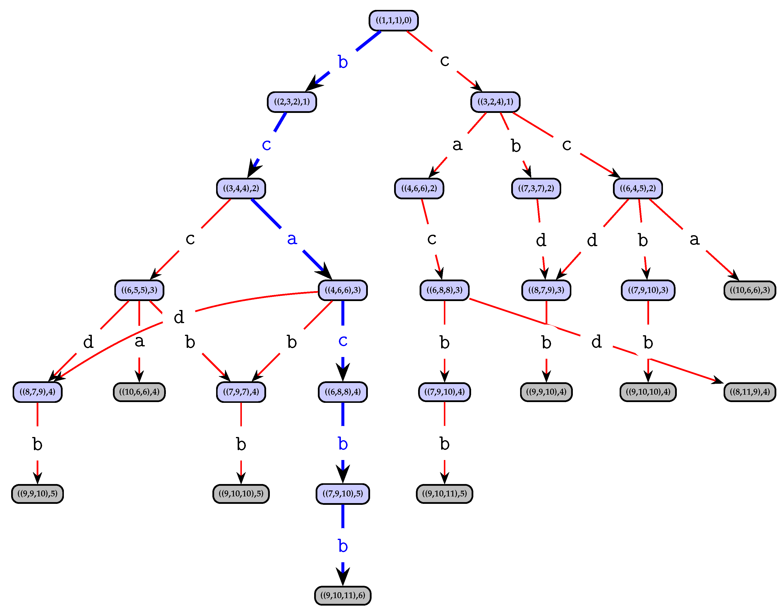
3.2. State Graph for the LCS Problem
The state graph for the LCS problem that is used by all BS variants is already well known in the literature, see, for example [
16,
24]. It is defined as a directed acyclic graph
, where a node
represents the set of partial solutions, which:
We say that a partial solution s induces a subproblem iff is the smallest prefix of among all prefixes that has s as a subsequence.
An arc exists between two nodes and carries label , iff
The root node of G refers to the original LCS problem on input string set S and can be said to be induced by the empty partial solution .
For deriving the successor nodes of a node
, we first determine the subset
of the letter that feasibly extends the partial solutions represented by
v. The candidates for letter
are therefore all letters
that appear at least once in each string in the subproblem given by strings
. This set
may be reduced by determining and discarding dominated letters. We say that letter
dominates letter
iff
Dominated letters can be safely omitted since they lead to suboptimal solutions. Let
be the set of feasible and non-dominated letters. For each letter
, graph
G contains a successor node
of
v, where
,
(remember that
denotes the position of the first appearance of letter
a in string
from position
onward). A node
v that has no successor node, that is, when
, is called a
non-extensible node, or
goal node. Among all goal nodes
v we are looking for one representing a longest solution string, that is, a goal node with the largest
. Note that any path from the root node
r to any node in
represents the feasible partial solution obtained by collecting and concatenating the labels of the traversed arcs. Thus, it is not necessary to store actual partial solutions
s in the nodes. In the graph
G, any path from root
r to a non-extensible node represents a common, non-extensible subsequence of
S. Any longest path from
r to a goal node represents an optimal solution to problem instance
S. As an example of a full state graph of an instance, see
Figure 1.
We still have to explain the filtering of dominated nodes from the set
, that is, procedure
Filter in Algorithm 1. We adopt the efficient
restricted filtering proposed in [
13], which is parameterized by a filter size
. The idea is to select only the (up to)
best nodes from
and to check the dominance relation (
6) for this subset of nodes in combination with all other nodes in
. If the relation is positively evaluated, the dominated node is removed from
. Note that parameter settings
and
represent the two extreme cases of no filtering and full filtering, respectively. A filter size of
may be meaningful, as full filtering may be too costly in terms of running time for larger beam widths.
3.3. Novel Heuristic Guidance
We now present a new heuristic for evaluating nodes in the BS in order to rank them and to select the beam of the next level. This heuristic, called the Geometric mean probability sum (Gmpsum), in particular aims at unbalanced instances and is a convex combination of the following two scores.
More specifically, for a given node
v and a letter
, let us define
as the vector indicating for each remaining string of the respective subproblem the number of occurrences of letter
. By
and
, we denote the geometric mean and geometric standard deviation, respectively, which are calculated for
by
By
, we denote the known upper bound on the length of an LCS for the subproblem represented by node
v from [
11], which is calculated as
Then, the
Gm score is calculated as
Overall, the Gm score is thus a weighted average of the adjusted geometric means ( of the number of letter occurrences, and the weight of each letter is determined by normalizing the minimal number of the letter occurrences across all strings with the sum of the minimal number occurrences across all letters. The motivation behind this calculation is three-fold:
Letters with higher average numbers of occurrences across the strings will increase the chance of finding a longer common subsequence (composed of these letters).
Higher deviations around the mean naturally reduce this chance.
The minimal numbers of occurrences of a letter across all input strings is an upper bound on the length of common subsequences that can be formed by this single letter. Therefore, by normalizing it with the sum of all minimal letter occurrences, an impact of each letter in the overall summation is quantified.
The Gm score is relevant if its underlying sampling geometric mean and standard deviation are based on a sample of sufficient size. In all our experiments, the minimal number of input strings is therefore ten. Working on samples of smaller sizes would likely make the Gm score not that useful.
In addition to the
Gm score, we consider the
Psum score. For a given node
v, we define
Then, the
Psum score is calculated by
Unlike the Gm score, which considers mostly general aspects of an underlying probability distribution, Psum better captures more specific relations among input strings. It represents the sum of probabilities that a string of length k will be a common subsequence for all remaining input strings relevant for further extensions. Index k goes from one to , that is, the length of the shortest possible non-empty subsequence up to the length of the longest possible one, which corresponds to the size of the shortest input string residual. The motivation behind using a simple (non-weighted) summation across all potential subsequence lengths is three-fold:
The exact length of the resulting subsequence is not known in advance. Note that, in the case of the
Hp heuristic proposed in [
12], the authors heuristically determine an appropriate value of
k for each level in the BS.
The summation across all k provides insight into the overall potential of node v—approximating the integral on the respective continuous function. Note that it is not required for this measure to have an interpretation in absolute terms since throughout the BS it is used strictly to compare different alternative extensions on the same level of the BS tree.
A more sophisticated approach that assigns different weights to the different k values would impose the challenge of deciding these specific weights. This would bring us back to the difficult task of an expected length prediction, which would be particularly hard when now considering the arbitrary multinomial distribution.
Finally, the total
Gmpsum score is calculated by the linear combination
where
is a strategy parameter. Based on an empirical study with different benchmark instances and values for parameter
, we came up with the following rules of thumb to select
.
Since Gm and Psum have complementary focus, that is, they capture and award (or implicitly penalize) different aspects of the extension potential, their combined usage is indeed meaningful in most cases, that is, .
Gm tends to be a better indicator when instances are more regular, that is, when each input string better fits the overall string distribution.
Psum tends to perform better when instances are less regular, that is, when input strings are more dispersed around the overall string distribution.
Regarding the computational costs of the
Gmpsum calculation, the
Gm score calculation requires
time. This can be concluded from (
7), where the most expensive part is the iteration through all letters from
and finding the minimal number of the letter occurrences across all
m input strings (
and
have the same time complexity). Note that the number of occurrences of each letter across all possible suffixes of all
m input string positions is calculated in advance, before starting the beam search, and is stored in an appropriate three-dimensional array, see [
24]. The worst case computational complexity of this step is
. This is because the number of occurrences of a given letter across all positions inside the given input string can be determined in a single linear pass. Since this is done only at the start, and the expected number of
Gm calls is much higher than
, this up front calculation can be neglected in the overall computational complexity The
Psum score given by (
8) takes
time to be calculated due to a definition of
. Similar to
Gm, the calculation of matrix
P is performed in pre-processing—its computational complexity corresponds to the number of entries, that is,
, see (
5).
Finally, the total computational complexity of Gmpsum can be concluded to be . The total computational complexity of the beam search is therefore a product of the number of calls of Gmpsum and the time complexity of Gmpsum. Note that the number of Gmpsum calls equals the number of nodes created within a BS run. Since the LCS length, that is, the number of BS levels, is unknown, we use here as the upper bound. Overall, the BS guided by Gmpsum runs in time if no filtering is performed. In the case of filtering, at each level of the BS, time is required, which gives total time for executing the filtering within the BS. According to this, the BS guided by Gmpsum and utilizing (restricted) filtering requires time.
3.4. A Time-Restricted BS
In this section, we extend the basic BS from Algorithm 1 to a time-restricted beam search (TRBS). This BS variant is motivated by the desire to compare different algorithms with the same time-limit. The core idea we apply is to dynamically adapt the beam width in dependence of the progress over the levels.
Similarly to the standard BS from Algorithm 1, TRBS is parameterized with the problem instance to solve, the guidance heuristic h, and the filtering parameter . Moreover, what was previously the constant beam width now becomes only the initial value. The goal is to achieve a runtime that comes close to a target time , now additionally specified as an input. At the end of each major iteration, that is, level, if , that is, the time limit is actually enabled, the beam width for the next level is determined as follows.
Let be the time required for the current iteration.
We estimate the remaining number of major iterations (levels) by taking the maximum of lower bounds for the subinstances induced by the nodes in
. More specifically,
Thus, for each node
and each letter
a we consider the minimal number of occurrences of the letter across all string suffixes
and select the one that is maximal. In other words, this LCS lower bound is based on considering all common subsequences in which a single letter is repeated as often as possible. In the literature, this procedure is known by the name
Long-run [
35] and provides a
–approximation.
Let be the actual time still remaining in order to finish at time .
Let be the expected remaining time when we would continue with the current beam width and the time spent at each level would stay the same as it was when measured for the current level.
(5)Depending on the discrepancy between the actual and expected remaining time, we possibly increase or decrease the beam width for the next level:
In this adaptive scheme, the thresholds for the discrepancy to increase or decrease the beam width, as well as the factor by which the beam width is modified, were determined empirically. Note that there might be better estimates of the LCS length than ; however, this estimate is inexpensive to obtain, and even if it underestimates or overestimates the LCS length in the early phases, gradually it converges toward the actual LCS length as the algorithm progresses. This allows TRBS to smoothly adapt its expected remaining runtime to the desired one. Note that we only adapt the beam width and do not set it completely anew based on the runtime measured for the current level in order to avoid erratic changes of the beam width in the case of a larger variance of the level’s runtimes. Based on preliminary experiments, we conclude that the proposed approach in general works well in achieving the desired time limit, while not changing dramatically up and down in the course of a whole run. However, of course, how close we get to the time limit being met depends on the actual length of the LCS. For small solution strings, the approach has fewer opportunities to adjust and then tends to overestimate the remaining time, thus utilizing less time than desired.
4. Experimental Results
In this section we evaluate our algorithms and compare them with the state-of-the-art algorithms from the literature. The proposed algorithms are implemented in C# and executed on machines with Intel i9-9900KF CPUs with @ 3.6 GHz and 64 Gb of RAM under Microsoft Windows 10 Pro OS. Each experiment was performed in single-threaded mode. We conducted two types of experiments:
short-runs: these are limited-time scenarios—that is, BS configurations with are used—executed in order to evaluate the quality of the guidance of each of the heuristics towards promising regions of the search space.
long-runs: these are fixed-duration scenarios (900 s) in which we compare the time-restricted BS guided by the Gmpsum heuristic with the state-of-the-art results from the literature. The purpose of these experiments is the identification of new state-of-the-art solutions, if any.
4.1. Benchmark Sets
All relevant benchmark sets from the literature were considered in our experiments:
4.2. Considered Algorithms
All considered algorithms make use of the state-of-the-art BS component. In order to test the quality of the newly proposed
Gmpsum heuristic for the evaluation of the partial solutions at each step of BS, we compared it to the other heuristic functions that were proposed for this purpose in the literature:
Ex [
16],
Pow [
13], and
Hp [
12]. The four resulting BS variants are labeled
BS-Gmpsum,
BS-Ex,
BS-Pow, and
BS-Hp, respectively. These four BS variants were applied with the same parameter settings (
and
) in the short-run scenario in order to ensure that all of them used the same amount of resources.
In the long-run scenario, we tested the proposed time-restricted BS (TRBS) guided by the novel
Gmpsum heuristic, which is henceforth labeled as
TRBS-Gmpsum. Our algorithm was compared to the current state-of-the-art approach from the literature:
+ ACS [
24]. These two algorithms were compared in the following way:
Concerning
+ ACS, the results for benchmark sets
Random,
Virus,
Rat,
Es and
Bb were taken from the original paper [
24]. They were obtained with a computation time limit of 900 s per run. For the new benchmark sets—that is,
Poly and
Bacteria—we applied the original implementation of
+ ACS with a time limit of 900 s on the above-mentioned machine.
TRBS-
Gmpsum was applied with a computation time limit of 600 s per run to all instances of benchmark sets
Random,
Virus,
Rat,
Es and
Bb. Note that we reduced the computation time limit used in [
24] by 50% because the CPU of our computer was faster than the one used in [
24]. In contrast, the time limit for the new instances was set to 900 s. Regarding restricted-filtering, the same setting (
) as for the short-run experiments was used.
4.3. Tuning of Parameter
As already mentioned in the previous section, the values of parameters
(beam width) and
(for filtering dominated nodes) were adopted from [
16] (for the short-run executions) and from [
24] (for the long-run executions). Regarding the strategy parameter
that controls the impact of both scores in the
Gmpsum score, we performed short-run evaluations across a discrete set of possible values:
. The conclusion was that the best performing values were
for
Bb,
for
Virus and
Bacteria,
for
Random,
Rat and
Poly, and
for
ES. The same settings for
were used in the context of the long-run experiments.The settings of the parameters of our algorithms BS-
Gmpsum and TRBS-
Gmpsum are displayed in
Table 1 and
Table 2.
4.4. Summary of the Results
Before studying the results for each benchmark set in detail, we present a summary of the results in order to provide the reader with a broad picture of the comparison. More specifically, the results of the short-run scenarios are summarized in
Table 3, while those for the long-run scenarios are given in
Table 4.
Table 3 displays the results in such a way that each line corresponds to a single benchmark set. The meanings of the columns are as follows: the first column contains the name of the benchmark set, while the second column provides the number of instances—respectively, instance groups—in the set. Then there are four blocks of columns, one for each considered BS variant. The first column of each block shows the obtained average solution quality (
) over all instances of the benchmark set. The second column indicates the number of instances—respectively, instance groups—for which the respective BS variant achieves the best result (#b.). Finally, the third column provides the average running time (
) in seconds over all instances of the considered benchmark set.
The following conclusions can be drawn:
Concerning the fully random benchmark sets Random and Es, in which input strings were generated uniformly at random and are independent, it was already well-known previously that the heuristic guidance Ex performs strongly. Nevertheless, it can be seen that BS-Gmpsum performs nearly as well as BS-Ex, and clearly better than the remaining two BS variants.
In the case of the quasi-random instances of benchmark sets Virus and Rat, BS-Gmpsum starts to show its strength by delivering the best solution qualities in 31 out of 40 cases. The second best variant is BS-Ex, which still performs very well, and is able to achieve the best solution qualities in 24 out of 40 cases.
For the special Bb benchmark set, in which input strings were generated in order to be similar to each other, Gmpsum was revealed to perform comparably to the best variant BS-Pow.
Concerning the real-world benchmark set Bacteria, BS-Gmpsum is able to deliver the best results for 18 out of 35 groups, which is slightly inferior to the BS-Hp variant with 22 best-performances, and superior to variants BS-Ex (12 cases) and BS-Pow (15 cases). Concerning the average solution quality obtained for this benchmark set, BS-Gmpsum is able to deliver the best among all considered approaches.
Concerning the multinominal non-uniformly distributed benchmark set Poly, BS-Gmpsum clearly outperforms all other considered BS variants. In fact, BS-Gmpsum is able to find the best solutions for all six instance groups. Moreover, it beats the other approaches in terms of the average solution quality.
Overall, BS-Gmpsum finds the best solutions in 80 (out of 121) instances or instance groups, respectively. The second best variant is BS-Ex, which is able to achieve the best performance in 62 cases. In contrast, BS-Hp and BS-Pow are clearly inferior to the other two approaches. We conclude that BS-Gmpsum performs well in the context of different letter distributions in the input strings, and it is worth trying this variant first when nothing is known about the distribution in the considered instance set.
Overall, the running times of all four BS variants are comparable. The fastest one is BS-Hp, while BS-Gmpsum requires somewhat more time compared to the others since it makes use of a heuristic function that combines two functions.
Table 4 provides a summary of the long-run scenarios, that is, it compares the current state-of-the-art algorithm
+ ACS with
TRBS-Gmpsum. As the benchmark instances are the same as in the short-run scenarios, the first two table columns are the same as in
Table 4. Then there are two blocks of columns, presenting the results of A* + ACS and
TRBS-Gmpsum in terms of the average solution quality over all instances of the respective benchmark set (
), and the number of instances (or instance groups) for which the respective algorithm archived the best result (#b.).
The following can be concluded based on the results obtained for the long-run scenarios:
Concerning Random and Es, + ACS is—as expected—slightly better than TRBS-Gmpsum in terms of the number of best results achieved. However, when comparing the average performance, there is hardly any difference between the two approaches: 109.9 vs. 109.7 for the Random benchmark set, and 243.82 vs. 243.73 for the Es benchmark set.
In the context of benchmark sets Rat and Virus, TRBS-Gmpsum improves over the state-of-the-art results by a narrow margin. This holds both for the number of best results achieved and for the average algorithm performance.
Concerning benchmark set Bb, TRBS-Gmpsum significantly outperforms + ACS. In six out of eight groups it delivers the best average solution quality, while + ACS does so only for three cases.
The same holds for the real-world benchmark set Bacteria, that is, TRBS-Gmpsum achieves the best results for 33 out of 35 instances, in contrast to only 10 instances in the case of A* + ACS. Moreover, the average solution quality obtained is much better for TRBS-Gmpsum, namely 862.63 vs. 829.26.
Finally, the performances of both approaches for benchmark set Poly are very much comparable.
Overall, we can conclude that TRBS-Gmpsum is able to deliver the best results in 101 out of 121 cases, while + ACS does so only in 77 cases. This is because TRBS-Gmpsum provides a consistent solution quality across instances characterized by various kinds of letter distributions. It can therefore be stated that TRBS-Gmpsum is a new state-of-the-art algorithm for the LCS problem.
In summary, for the 32 random instances—respectively, instance groups—from the literature (sets Random and Es) + ACS performs quite strongly due to the presumed randomness of the instances. However, the new TRBS-Gmpsum approach is not far behind. A weak point of + ACS becomes obvious when instances are not generated uniformly at random. In the 40 cases with quasi-random input strings (sets Rat and Virus), TRBS-Gmpsum performs the best in 37 cases, while + ACS does so in 31 cases. When input strings are similar to each other—see the eight instance groups of set Bb— + ACS performs weakly compared to TRBS-Gmpsum. This tendency is reinforced in the context of the instances of set Poly (six instance groups) for which TRBS-Gmpsum clearly outperforms + ACS in all cases. The same holds for the real-world benchmark set Bacteria. The overall conclusion yields that TRBS-Gmpsum works very well on a wide range of different instances. Moreover, concerning the instances from the previous literature (80 instances/groups), our TRBS-Gmpsum approach is able to obtain new state-of-the-art results in 13 cases. This will be shown in the next section.
4.5. New State-of-the-Art Results for Instances from the Literature
Due to space restrictions, we provide the complete set of results for each problem instance in the Supplementary Materials of the repository whose the link is given in the Data Availability Statement at the end of the paper.
The tables reporting the new state-of-the-art results are organized as follows. The first column contains the name of the corresponding benchmark set, while the following two columns identify, respectively, the instance (in the case of Rat and Virus) and the instance group (in the case of Bb and Es). Afterwards, there are two columns that provide the best result known from the literature. The first of these columns provides the result, and the second column indicates the algorithm (together with the reference) that was the first one to achieve this result. Next, the tables provide the results of Bs-Ex, Bs-Pow, Bs-Hp and Bs-Gmpsum in the case of the short-run scenario, the results of A* + ACS and TRBS-Gmpsum, respectively, in the case of the long-run scenario. Note that computation times are only given for the short-run scenario, because time served as a limit in the long-run scenario.
Concerning the short-run scenario (
Table 5),
BS-Gmpsum was able to produce new best results in 17 cases. This even includes four cases of the benchmark set
Es, which was generated uniformly at random. The four cases of sets
Virus and
Rat are remarkable, in which the currently best-known solution was improved by two letters (see, for example, the case of set
Rat and the instance
,
and
). Concerning the more important long-run scenario (
Table 6), the best-known results so far were improved in 14 cases. Especially remarkable is the case of set
Bb, for which an impressive improvement of around 24 letters was achieved.
4.6. Results for Benchmark Sets Poly and Bacteria
The tables reporting the results for benchmark set Poly are structured in the same way as those described above in the context of the other benchmark sets. The difference is that instance groups are identified by means of (first column), m (second column), and n (third column). The best results per instance group—that is, per table row—are displayed in bold font.
The results of the short-run scenario for benchmark set
Poly are given in
Table 7. According to the obtained results, a clear winner is
BS-Gmpsum, which obtains the best average solution quality for all six instance groups. This indicates that
Gmpsum is clearly better as a search guidance than the other three heuristic functions for this benchmark set. As previously mentioned, this is due to the strongly non-uniform nature of the instances, that is, the intentionally generated imbalance of the number of occurrences of different letters in the input strings. Nevertheless, the absolute differences between the results of
BS-Gmpsum and
BS-Ex are not so high. The results of the long-run executions for benchmark set
Poly are provided in
Table 8. It can be observed that
TRBS-Gmpsum and the state-of-the-art technique A* + ACS perform comparably.
Remember that, as in the case of
Poly, the instances of benchmark set
Bacteria have been used for the first time in a study concerning the LCS problem. They were initially proposed in a study concerning the constrained LCS problem [
39]. The results are again presented in the same way as described before. This set consists of 35 instances. Therefore, each line in
Table 9 (short-run scenario) and
Table 10 (long-run scenario) deals with one single instance, which is identified by
(always equal to 4),
m (varying between 2 and 383),
(the length of the shortest input string) and
(the length of the longest input string). The best results are indicated in bold font. The results obtained for the short-run scenario allow us to observe that
BS-Hp performs very well for this benchmark set. In fact, it obtains the best solution in 22 out of 35 cases. However,
BS-Gmpsum is not far behind with 18 best solutions. Moreover,
BS-Gmpsum obtains a slightly better average solution quality than
Bs-Hp. Concerning the long-run scenario, as already observed before,
TRBS-Gmpsum clearly outperforms A* + ACS. In fact, the differences are remarkable in some cases, such as, for example, instance number 32 (fourth but last line in
Table 10) for which
TRBS-Gmpsum obtains a solution of value 1241, while A* + ACS finds—in the same computation time—a solution of value 1204.
4.7. Statistical Significance of the So-Far Reported Results
In this section, we study the results of the short-run and long-run executions from a statistical point of view. In order to do so, Friedman’s test was performed simultaneously considering all four algorithms in the case of the short-run scenario, and the two considered algorithms in the case of the long-run scenario. All these tests and the resulting plots were generated using
R’s scmamp package [
41].
Given that, in all cases, the test rejected the hypothesis that the algorithms perform equally, pairwise comparisons were performed using the Nemenyi post-hoc test [
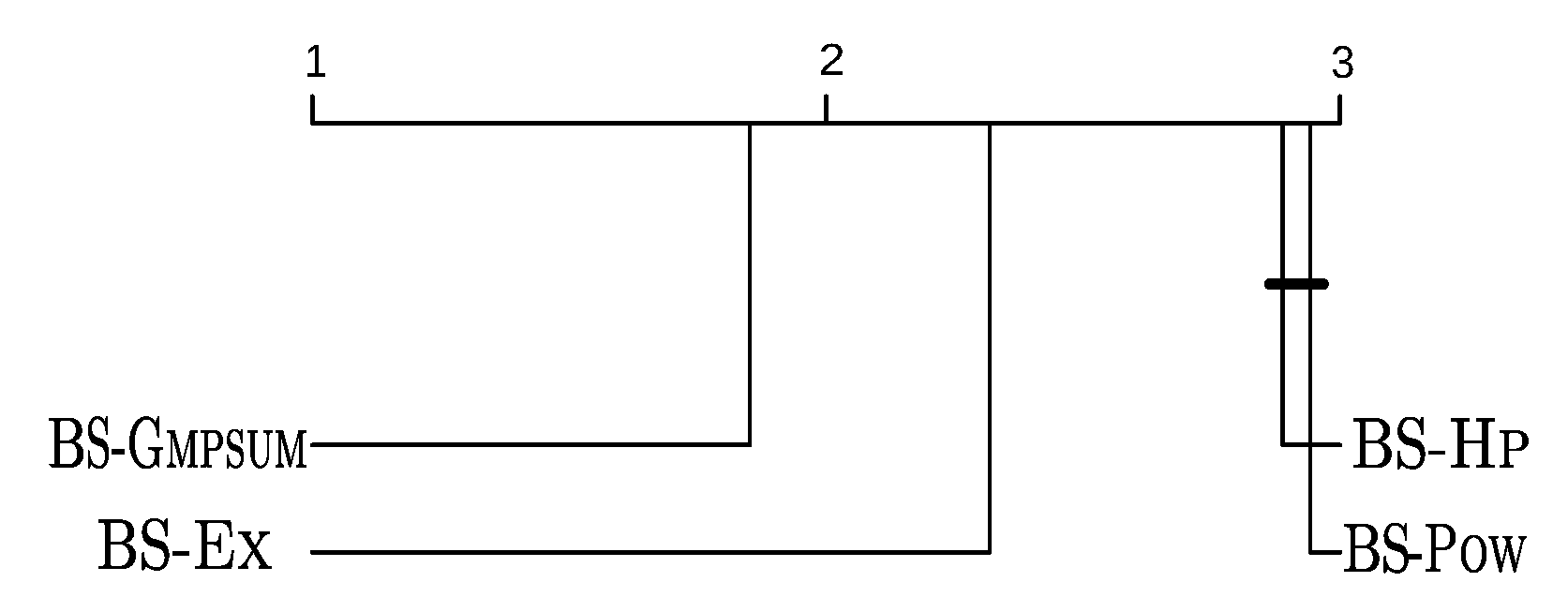
42]. The corresponding critical difference (CD) plots considering all benchmark sets together are shown in
Figure 2 and
Figure 3a. Each algorithm is positioned in the segment according to its average ranking with regard to the average solution quality over all (121) the considered instance groups. The critical difference was computed with a significance level of 0.05. The performances of those algorithms whose difference is below the CD are regarded as performing statistically in an equivalent way—that is, no difference of statistical significance can be detected. This is indicated in the figures by bold horizontal bars joining the respective algorithm markers.
Concerning short-run executions, BS-
Gmpsum is clearly the overall best-performing algorithm, with statistical significance. BS-
Ex is in the second position. Moreover, the difference between BS-
Hp and BS-
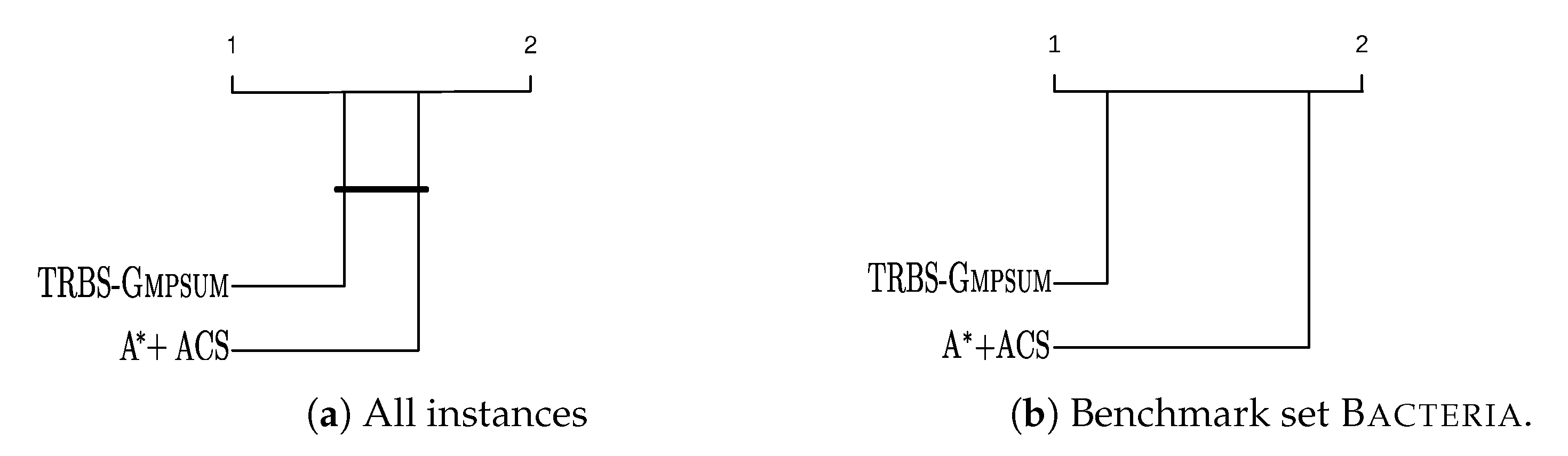
Pow is not statistically significant. Concerning the long-run scenario, the best average rank is obtained by TRBS-
Gmpsum. In the case of benchmark set
Bacteria, the difference between TRBS-
Gmpsum and
+ ACS is significant, see
Figure 3b. For the other benchmark sets, the two approaches perform statistically equivalently.
5. Textual Corpus Case Study
In the previous section, we showed that the proposed method is highly competitive with state-of-the art methods and generally outperforms them on instances sampled from non-uniform distributions. In order to further investigate the behavior of the proposed method in real-world instances with non-uniform distribution, we performed a case study on a corpus of textual instances originating from abstracts of scientific papers written in English. This set will henceforth be called
Abstract. It is known that letters in the English language are polynomially distributed [
28]. The most frequent letter is
e, with a relative frequency of 12.702%. The next most common letter is
t (9.056%), followed by
a (8.167%), and
o (7.507%), and so forth.
In order to make a meaningful choice of texts we followed [
43], where the authors measured the similarity between scientific papers, mainly from the field of artificial intelligence, by making use of various algorithms and metrics. By using tf-idf statistics with cosine similarity, their algorithm identified similar papers from a large paper collection. After that, the similarity between the papers proposed by their algorithm was manually checked and tagged by an expert as either similar (positive) or dissimilar (negative). The results of this research can be found at
https://cwi.ugent.be/respapersim (accessed on 14 March 2021).
Keeping in mind that the LCS problem is also a measure of text similarity, we decided to check whether the abstracts of similar papers have longer common subsequences than abstracts of dissimilar papers. Therefore, the purpose of this case study is twofold: (1) to execute the LCS state-of-the art methods along with the method proposed in this paper and to compare their performances on this specific instance set; and (2) to check whether the abstracts of similar papers have a higher LCS than those of dissimilar papers.
Based on these considerations, we formed two groups of twelve papers each, named POS and NEG. Group POS contains twelve papers which were identified as similar, while group NEG contains papers which are not similar to each other. We extracted abstracts from each paper and pre-processed them in order to remove all letters except for those letters from the English alphabet. In addition, each uppercase letter was replaced with its lowercase pair.
For each of the two groups, we created a set of test instances as follows. For each we generated different instances containing k input strings (considering all possible combinations). This resulted in the following set of instances for both POS and NEG:
One instance containing all 12 abstracts as input strings.
Twelve instances containing 11 out of 12 abstracts as input strings.
Sixty-six instances containing 10 out of 12 abstracts as input strings.
Repeating our experimental setup presented in the previous section, we performed both short- and long-runs for the described instances. The obtained results for the short-run scenarios are shown in
Table 11. The table is organized into five blocks of columns. The first block provides general information about the instances:
NEG vs.
POS, number of input strings (column with heading
m), and the total number of instances (column #). The remaining four blocks contain the results of BS-
Ex, BS-
Pow, BS-
Hp and BS-
Gmpsum, respectively. For each considered group of instances and each method, the following information about the obtained results is shown:
: solution quality of the obtained LCS for the considered group of instances;
#b.: number of cases in which the method reached the best result for the considered group of instances;
: average execution time in seconds for the considered group of instances.
The results from
Table 11 clearly indicate that the best results for instances based on group
NEG are obtained by BS-
Gmpsum. More precisely, BS-
Gmpsum works best for the instance with 12 input strings, for eight out of 12 instances with 11 input strings and for 50 out of 66 instances with 10 input strings. In contrast, the second-best approach (BS-
Ex) reached the best result for 29 out of 66 instances with 10 input strings and seven out of 12 instances with 11 input strings. The remaining two methods were less successful for this group of instances. For the instances derived from group
POS, BS-
Gmpsum also achieved very good results. More specifically, BS-
Gmpsum obtained the best results in almost all instances with 11 input strings. For instances with 10 input strings, BS-
Ex obtained the best results in 42 out of 66 cases, with BS-
Gmpsum performing comparably (best result in 39 out of 66 cases). For the instance with 12 strings, the best solution was found by the BS-
Ex. Similarly to the instances from the
NEG group, BS-
Hp and BS-
Pow are clearly less successful.
A summary of these results is provided in the last three rows of
Table 11. Note that, in total, this table deals with 158 problem instances: 79 regarding group
NEG, and another 79 regarding group
POS. The summarized results show that the new
Gmpsum guidance is, overall, more successful than its competitors. More precisely, BS-
Gmpsum achieved the best results in 59 out of 79 cases concerning
NEG, and in 50 out of 79 cases concerning
POS. Moreover, it can be observed that the average LCS length regarding the
POS instances is greater than that regarding the
NEG instances, across all
m values.
Table 12 contains information about the long-run executions. The results obtained by
+ ACS and TRBS-
Gmpsum are shown. The table is organized in a similar way to
Table 11, with the exception that it does not contain information about execution times, since computation time served as the stopping criterion. As can be seen from the overall results at the bottom of Table, TRBS-
Gmpsum obtains more best results than
+ ACS for both groups of instances (
NEG and
POS). More precisely, it obtained the best result for the instances with 12 input strings, both in the case of
POS and
NEG, while A* + ACS achieved the best result only in the case of the
POS instance with 12 input strings. Concerning the results for the instances with 11 input strings, it can be noticed that—in the case of the
NEG instances—TRBS-
Gmpsum delivers 11 out of 12 best results, while the
+ ACS method does so only in two out of twelve cases. Regarding the
POS instances with 11 input strings, the difference becomes smaller. More specifically, TRBS-
Gmpsum achieves nine out of 12 best results, while
+ ACS achieved six out of 12 best results. A corresponding comparison can be made for the instances with 10 input strings. For the instances concerning group
NEG, TRBS-
Gmpsum delivers the best results for 60 out of 66 instances, while
+ ACS can find the best results only in 31 cases. Finally, in the case of the
POS instances, the best results were achieved in 45 out of 66 cases by TRBS-
Gmpsum, and in 41 out of 66 cases by
+ ACS. The long-run results also indicate that abstracts of similar papers are characterized by generally longer LCS measures.
6. Conclusions and Future Work
In this paper, we considered the prominent longest common subsequence problem with an arbitrary set of input strings. We proposed a novel search guidance, named Gmpsum, for tree search algorithms. This new guidance function was defined as a convex combination of two complementary heuristics: (1) the first one is suited for instances in which the distribution of letters is close to uniform-at-random; and (2) the second is convenient for all cases in which letters are non-uniformly distributed. The combined score produced by these two heuristics provides a guidance function which navigates the search towards promising regions of the search space, on a wide range of instances with different distributions. We ran short-run experiments in which beam search makes use of a comparable number of iterations under different guidance heuristics. The conclusion was that the novel guidance heuristic performs statistically equivalently to the best-so-far heuristic from the literature on close-to-random instances. Moreover, it was shown that it significantly outperforms the known search guidance functions on instances with a non-uniform letter frequency per input string. This capability of the proposed heuristic to deal with a non-uniform scenario was validated on two newly introduced benchmark sets: (1) Poly, whose input strings are generated from a multinomial distribution; and (2) Abstract, which are real-world instances whose input strings follow a multinomial distribution and originate from abstracts of scientific papers written in English. In a second part of the experimentation, we performed long-run executions. For this purpose we combined the Gmpsum guidance function with a time-restricted BS that dynamically adapts its beam width during execution such that the overall running time is very close to the desired time limit. This algorithm was able to significantly outperform the best approach from the literature ( + ACS). More specifically, the best-known results from the literature were at least matched for 63 out of the 80 considered instance groups. Moreover, regarding the two new benchmark sets (Poly and Bacteria), the time-restricted BS guided by Gmpsum was able to deliver solutions that were equally as good as, and in most cases better than, those of + ACS, in 38 out of 41 instance groups.
In future work we plan to adapt
Gmpsum to other LCS-related problems such as the constrained longest common subsequence problem [
44], the repetition-free longest common subsequence problem [
45], the LCS problem with a substring exclusion constraint [
46], and the longest common palindromic subsequence problem [
47]. It would also be interesting to incorporate this new guidance function into the leading hybrid approach
+ ACS to possibly further boost the obtained solution quality.


 ,
, 


