Article

Electrical Model for Analyzing Chemical Kinetics, Lasing and Bio-Chemical Processes

1
School in Advanced Optical Technologies (SAOT), Friedrich-Alexander University of Erlangen-Nuremberg, Erlangen 91052, Germany
2
Faculty of Engineering, Bar-Ilan University, Ramat-Gan 52900, Israel
3
Nanotechnology Research Center, Bar-Ilan University, Ramat-Gan 52900, Israel
*
Author to whom correspondence should be addressed.
Processes 2013, 1(1), 12-29; https://doi.org/10.3390/pr1010012
Submission received: 5 February 2013 / Revised: 8 April 2013 / Accepted: 26 April 2013 / Published: 16 May 2013

Abstract

:
In this paper we present the analogous electrical model for analyzing and determining the precise time dependence of concentrations in general first and zero order chemical reactions. In addition, the applicability of this analogous electrical model for investigating the optical and bio chemical processes is also presented. By constructing the proper analogous electrical circuit experimentally or with the help of special electrical software, the time behavior of the analyzed parameter even for extremely complicated processes can be obtained.

1. Introduction

The kinetics of chemical reactions is usually described by a set of differential equations where the rate of the reaction is a function of concentration. The general form is defined by [1]:
Processes 01 00012 i001
where r is the rate (the time derivative of the concentration), c is the concentration, n is a constant named the reaction order and k is the rate constant. The multiplication index j is related to the number of components taking part in the reaction and the summation index l is related to the number of possible chemical combinations. The rate equation can be used to analyze a temporal progress of a chemical kinetic reaction and to define, for instance the concentrations or pressures values taking part within the reaction chain. Most of the kinetic reactions can be decomposed using a much simpler equations than the general form and accept the behavior of the first and second orders differential equations or a set of such equations. The simple linear differential equations are very easy to solve, but a set of inter connected differential equations, which represent a series of reactions that might be in equilibrium, can pose a serious obstacle for a solution [1,2]. However, the analogous approach can be applied for solving this case, whereas each component of the analyzed system is represented by a single electrical element. This appropriate element is selected in such a way that its voltage-current graph is similar to the velocity graph of the chemical concentration counterpart (including the differential relations). Such an approach had been tested before on mechanical, hydraulic [3], thermodynamics systems [4,5], Proton Electron Membrane (PEM) fuel cells [6] as well as on conducting polymer electrodes in electrolyte solutions [7].
In this paper, we present how a voltage can be used as analogous, among other for analyzing the concentration of chemical kinetic reactions either by building a compatible electrical circuit and measuring its output voltage time behavior or by using special electrical software [8]. By that, one may know the time behavior of the concentration, at the equivalent chemical kinetics reaction. A simulation tool such as PSpice software offers a friendly interface in which one may choose different electrical elements (i.e., power/current sources, dependent sources, resistors and capacitors) and drop them along the interface, while properly connecting them to each other. Then, the values of each electrical element in the circuit should be defined. Finally, voltage/current probes should be placed at points of interest along the circuit, whereas the simulation results will appear in a graph indicating the voltage/current as a function of time at all indicated probes.
In addition, the analogous electrical model can be adapted also to other fields such as the rate equation of atoms concentrations in laser as well as to investigate the time dependence of concentration in biological and biochemical problems which are usually very difficult issue to handle. In order to solve those problems a steady state assumption must be used [9,10]. Applying the suggested model, for this type of reactions will generate the time dependence of the concentrations without any assumptions. Please note that the proposed analogous electrical model is linear and simple and thus it is suitable for analyzing zero or first orders chemical kinetic reactions.
Moreover, If a scientist would like to investigate a physical or chemical processes whose parameters are unknown, he can build an analogous electrical circuit and study the output of this circuit by changing the value of one of its components (as a resistor). The output voltage (which is analogous to the examined parameter) will be obtained as fast as the speed of light. On the other hand, the scientist may use the “hardware solution” of the analogous electrical model in order to either learn about the behavior of differential equations having one or more symbolic parameters (i.e., one or more of the process parameters are unknown) or to avoid the computational cost caused by solving complicated equations. In Section 2 we present the simulation modeling of the analogous electrical model, while in Section 3 we present the results and discussions. The paper is concluded in Section 4.

2. Simulation Modeling

In this section, we present the analogous quantities of the electrical model related to the chemical kinetic equations. The solution of the electrical circuit is achieved either by proper electrical simulation software or by building the circuit experimentally and measuring its output. This procedure provides a precise solution of the material concentrations as a function of time in the examined chemical reaction. The proposed analogous model, described by Equations (2–6) defines the chemical components (i.e., left side of the equations) versus its analogous electrical elements (i.e., right side of the equations) is as following:
c, [A] ⇔ V
Processes 01 00012 i002
mq
V0C
V0vi
where, c is concentration in general and [A] is concentration of material A in moles per unit volume, V is the voltage, k is the reaction rate constant, R is the electrical resistance, C is the capacitance, m is the amount of moles, q is the electrical charge, V0 is the volume of the reaction, v is the reaction’s velocity which is equal to v = d[A]/dt and i presents the current.
At first, we should examine the consistency of this analogous electrical model where:
Processes 01 00012 i003
By applying the analogous model one may derive:
Processes 01 00012 i004
And this corresponds to the basic relation of a capacitor. Another example for the consistency of this model is:
Processes 01 00012 i005
This relation equals to the definition of an electrical current. By applying the model one obtains that:
Processes 01 00012 i006
Since V0 is a constant, this relation can be rewritten as:
Processes 01 00012 i007
Indeed this is the definition of the reaction’s velocity. Thus, it may be concluded that chemical kinetic reactions can be represented by a simple capacitor–resistor circuit, which is very simple to solve. By measuring or calculating a certain voltage over an electrical parameter, one may know the behavior of the materials concentration as a function of time at the required examined chemical component.
Figure 1 presents the analogous model for the most general first order reactions (i.e., reactions whose differential equation is linear). The analogous circuit should be drawn according to the following rules:
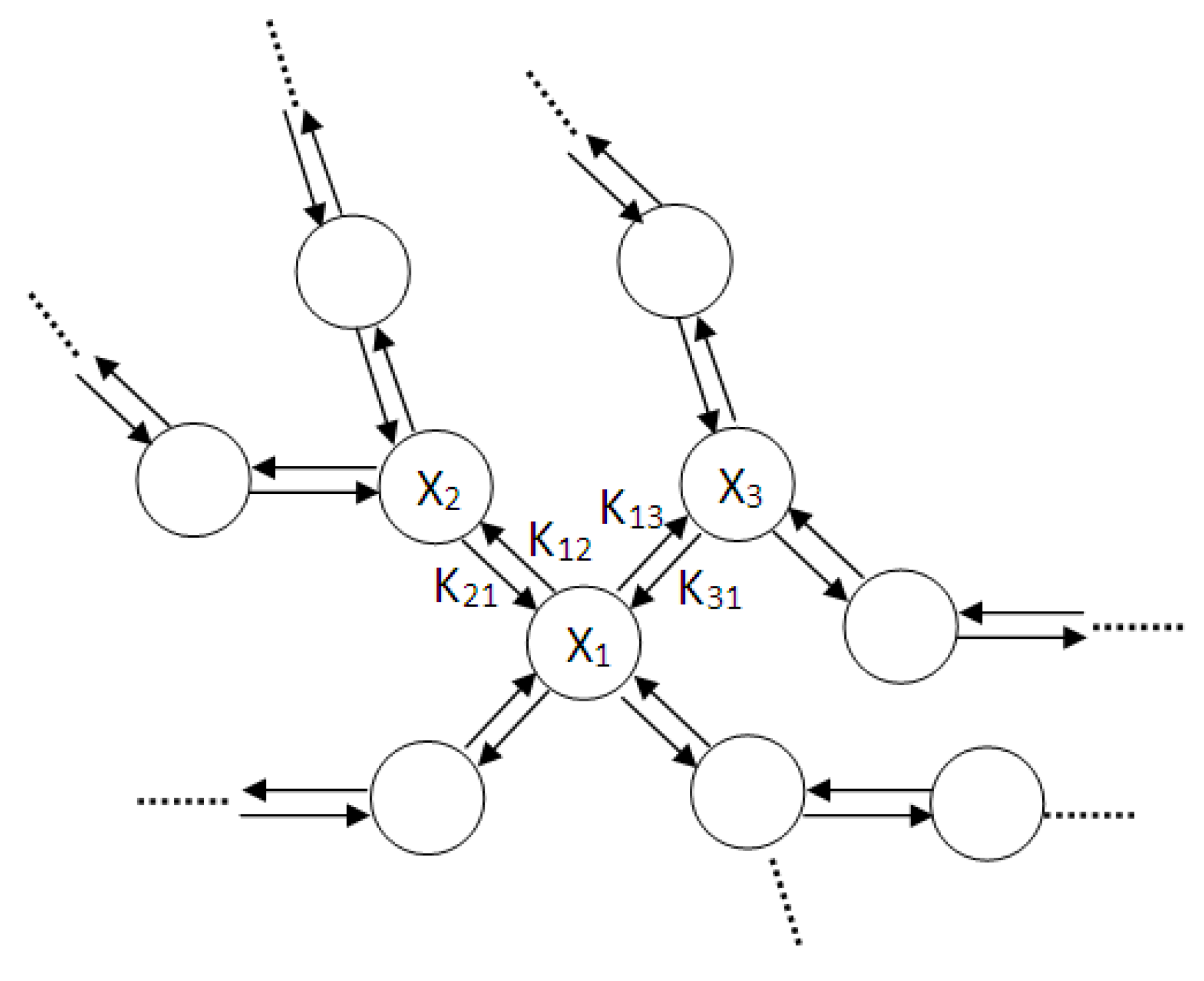
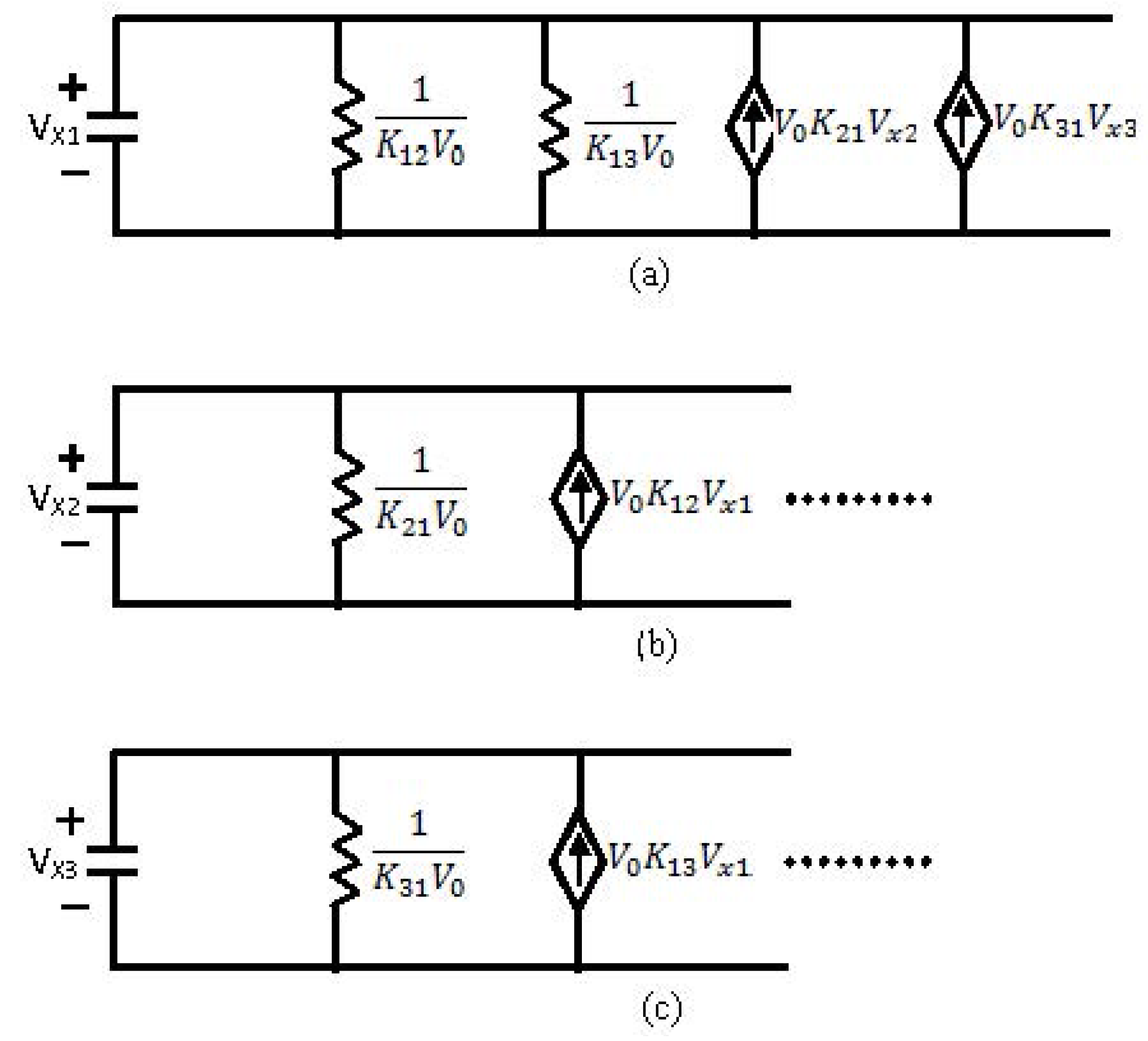
  • For each chemical element a different analogous circuit should be drawn.
  • The circuit is drawn only according to the chemical reaction equations.
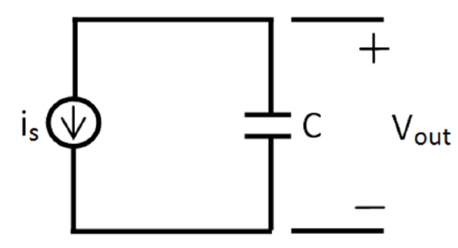
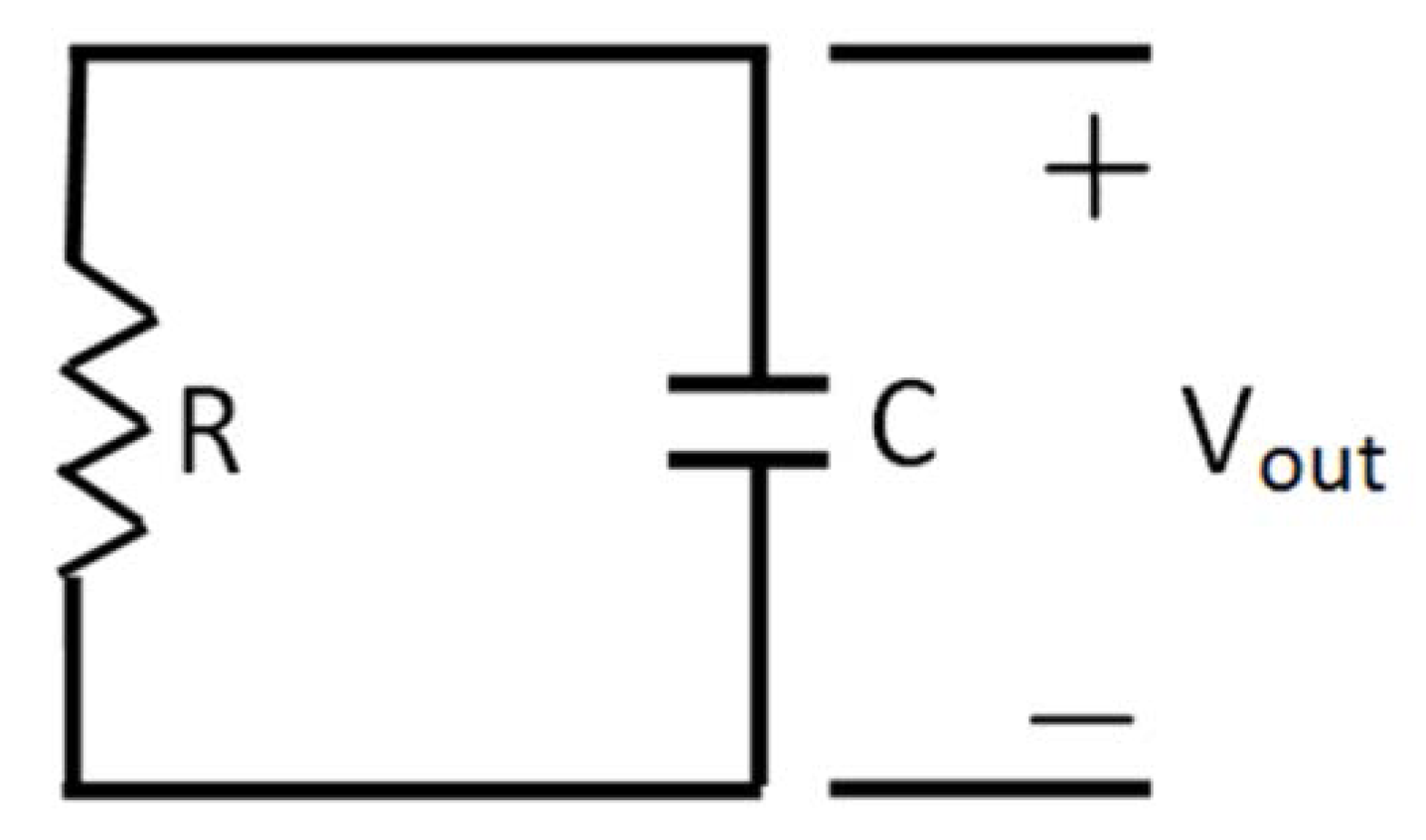
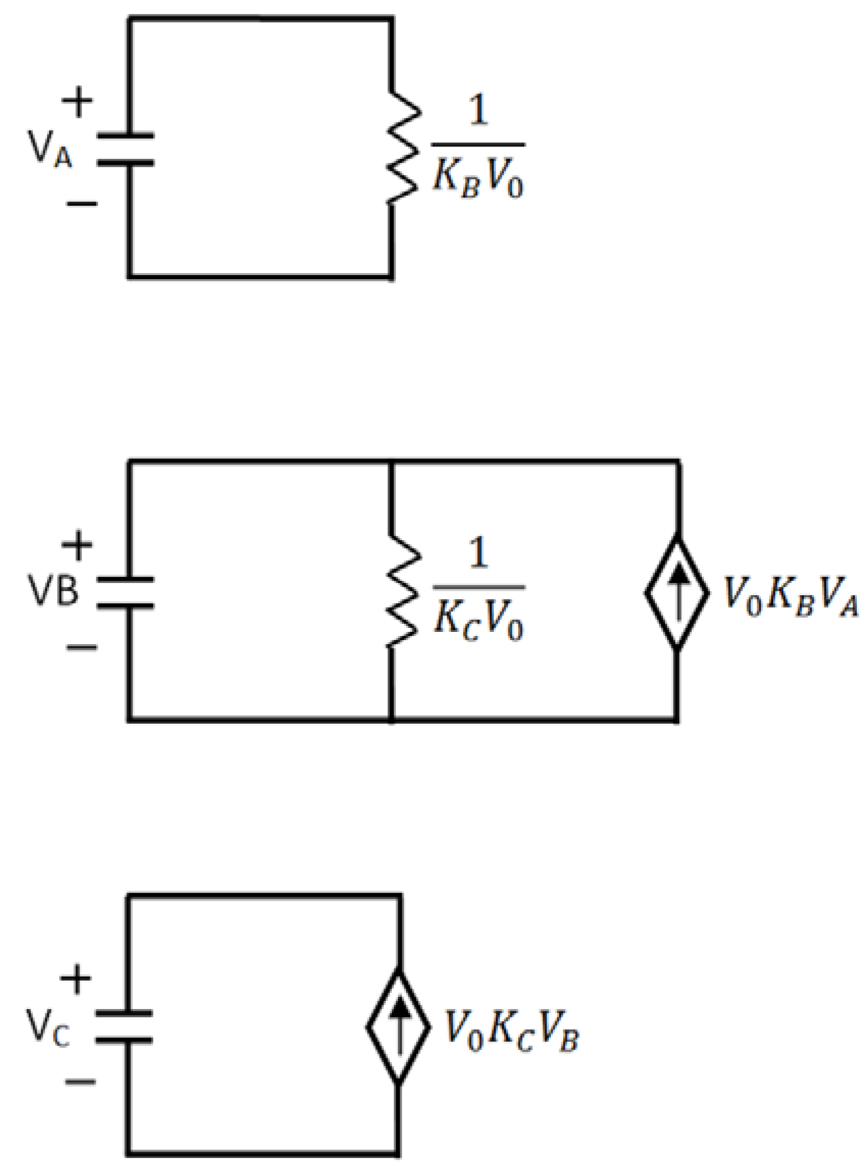
  • First a capacitor is drawn. The voltage upon this capacitor (VC) will be analogous to the concentration of the certain element.
  • Each arrow getting out of this element in its chemical reaction equation will be represented by a resistance in parallel to the capacitor. This is because each resistance is drawing current from the capacitor, an effect that is analogous to the “chemical current drawing”, i.e., the decomposition of one element and the creation of a new one. The value of each such resistance is Processes 01 00012 i008.
  • Each arrow pointing toward our element will correspond to a controlled current source, parallel to the resistance and the capacitor. Each current source like this will provide current to the capacitor, a phenomenon that is analogous to “chemical reaction” supplied by the decomposing element for the creation of a new element. The value of the current will be kiVi which is written in the base of this arrow while pointing toward the new element.
Figure 1. A sketch of the most general first order chemical kinetic reaction.
Processes 01 00012 g001
In Figure 2 we present the analogous electrical circuit corresponds to the most general first order chemical reaction shown in Figure 1. Figure 2a presents the analogous electrical model for the chemical reaction of element X1, while Figure 2b,c present the analogous electrical model for the chemical reactions of elements X2 and X3, respectively. Please note, that the symbol of the current source represents a controlled current source. This current source is proportional to a voltage applied at different branch along the circuit.
Figure 2. The analogous electrical circuits correspond to the most general first order reaction. (a) Analogous electrical model for chemical reaction of element X1. (b) and (c) analogous electrical model for chemical reactions of elements of X2 and X3, respectively.
Processes 01 00012 g002

3. Results and Discussion

3.1. Chemical Kinetics Reactions

In order to substantiate the theory, we examined the applicability of the proposed method in the most common chemical reactions based on the analogous relations presented by Equations (2–6). Figure 3 shows the analogous electrical circuit corresponds to the zero order chemical kinetic reaction.
Figure 3. The analogous electrical circuit for zero order reactions.
Processes 01 00012 g003
The electrical solution for this circuit is:
Processes 01 00012 i009
Thus
Processes 01 00012 i010
where Vout(t) is the desired output and Vc,o is the initial voltage on the capacitor. After applying the analogous model, Vout(t) corresponds to the concentration [A] and Vc,0 corresponds to the initial concentration of the decomposing material, thus:
[A] = [A]0kt
According to the dimensional analysis of the analogous model, the dimensions of k and Processes 01 00012 i011 are compatible. In addition, since Processes 01 00012 i012 the units of k and v are the same and equal to the chemical reaction velocity (i.e., concentration/time).
In Figure 4 we present the analogous electrical circuit corresponds to the first order reactions.
Figure 4. The analogous electrical circuit for the first order reactions represented by a resistor-capacitor circuit.
Processes 01 00012 g004
The solution of this electrical circuit is:
Processes 01 00012 i013
Which is exactly the solution for the first order reaction that equals to:
[A] = [A]0e−kt
Figure 5 presents the analogous electrical circuit corresponds to the reversible reactions.
Figure 5. The analogous electrical circuit for reversible reactions.
Processes 01 00012 g005
Where, Vin is analogous to the initial concentrations of A and B.
Vin ⇔ [A]0 + [B]0
The differential equation describes the electrical circuit of Figure 5 is:
Processes 01 00012 i014
Using the analogous table one may see that:
Processes 01 00012 i015
Processes 01 00012 i016
Thus, Equation (18) is exactly identical to the differential equation of the reversible chemical reaction and therefore the analogous solution is identical as well. Thus the solution is:
Processes 01 00012 i017
Therefore, the equilibrium constant in this case is equal to:
Processes 01 00012 i018
From Equations (21) and (22) for t→ ∞ one may get:
Processes 01 00012 i019
Thus, the equilibrium constant converges to the analogous constant of the electric circuit. The voltages of VB and VC represent the analogous time behavior for the concentration of material B ([B]) and A ([A]), respectively. One may see, that this circuit represents a more generalized case than the previous one. For the case where Rb→ ∞ (i.e., for kb = 0, the reaction becomes Processes 01 00012 i020) and there is a complete converges to the first order reaction (as seen in the previous model shown in Figure 4).
A triple consecutive reaction described by Processes 01 00012 i021 
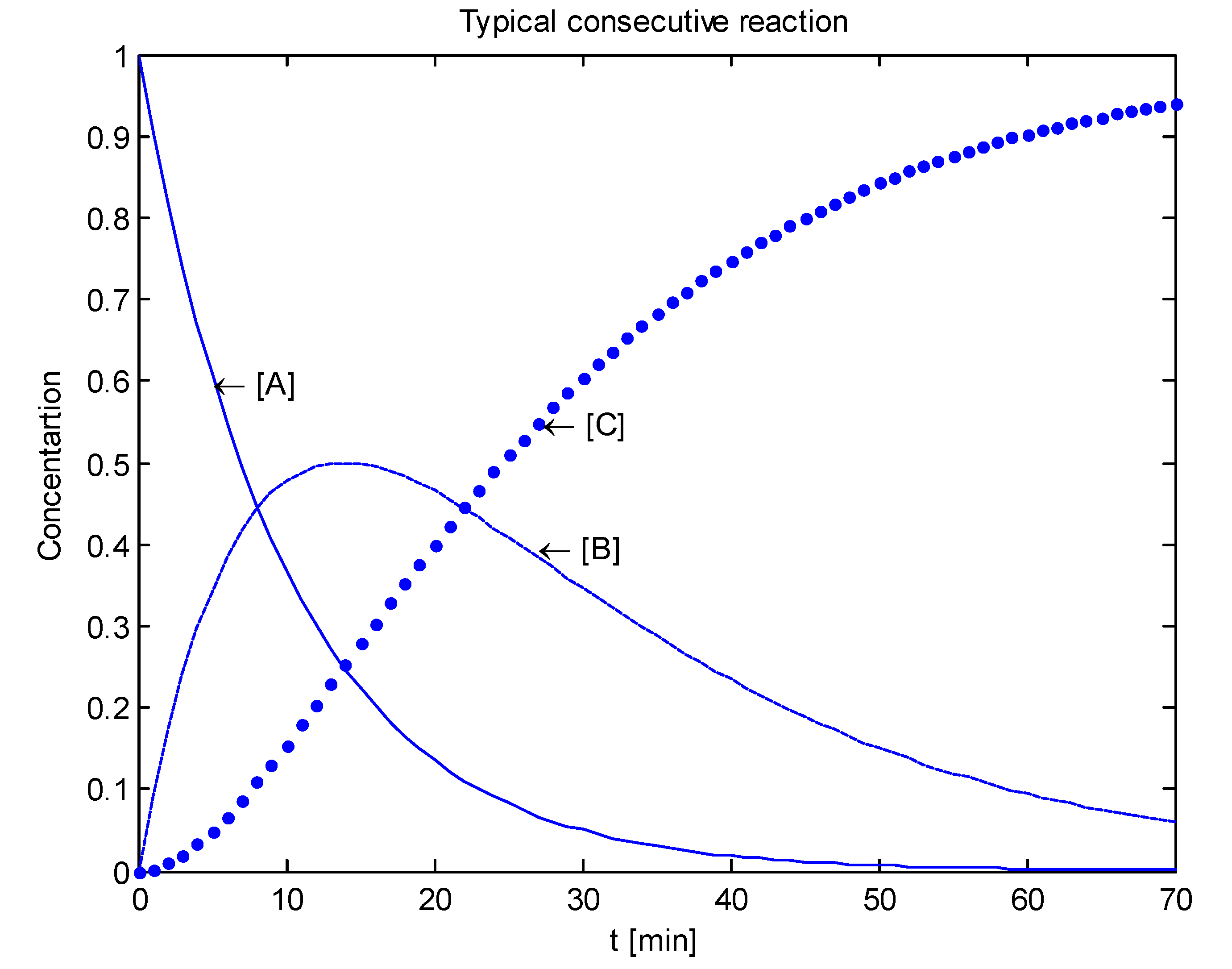
has been chosen. The reaction constants used in the simulations are: kb = 0.1 [min−1], kc = 0.05 [min−1], [A]0 = 1, [B]0 = 0, [C]0 = 0. Figure 6 shows the analogous electrical circuit used for this reaction. VA, VB and VC are the analogous voltages of concentrations [A], [B] and [C], respectively. The circuit is designed according to Figure 1, Figure 2. The output of the electrical simulation software is shown in Figure 7. The solid line presents the concentration of element A, while the dashed and the dotted lines present the concentrations of elements, B and C, respectively. According to [1], one may see the complete compatibility between the desired output and simulation results.
Figure 6. The analogous electrical circuit describing a triple consecutive reaction of concentrations [A], [B] and [C] used in the simulation software.
Processes 01 00012 g006
Figure 7. The output voltage (i.e., concentration) of elements [A], [B] and [C] as function of time.
Processes 01 00012 g007
In [2] an experimental data was given for the vapor phase decomposition of ethylene oxide into methane and carbon monoxide at 414.5° c is shown in Scheme 1.
Scheme 1. Vapor phase decomposition of ethylene oxide into methane and carbon monoxide.
Processes 01 00012 g016
The given data is related to the total pressure dependence upon time and since the reaction takes place in a vapor phase one may apply the ideal gas law:
PV = nRT
P = cRT
where, P is the pressure, c is the concentration, T is the temperature and R is related to the gas constant. Thus, the total pressure is proportional to the total concentration. The model shown in Figure 4 was constructed and the concentrations of CH4 and CO (the voltages that correspond to CH4 and CO elements) were added. The obtained total pressure is:
P(t) = P0e−kt + 2P0(1 − e−kt) = P0(2 − e−kt)
The rate constant k Processes 01 00012 i022 
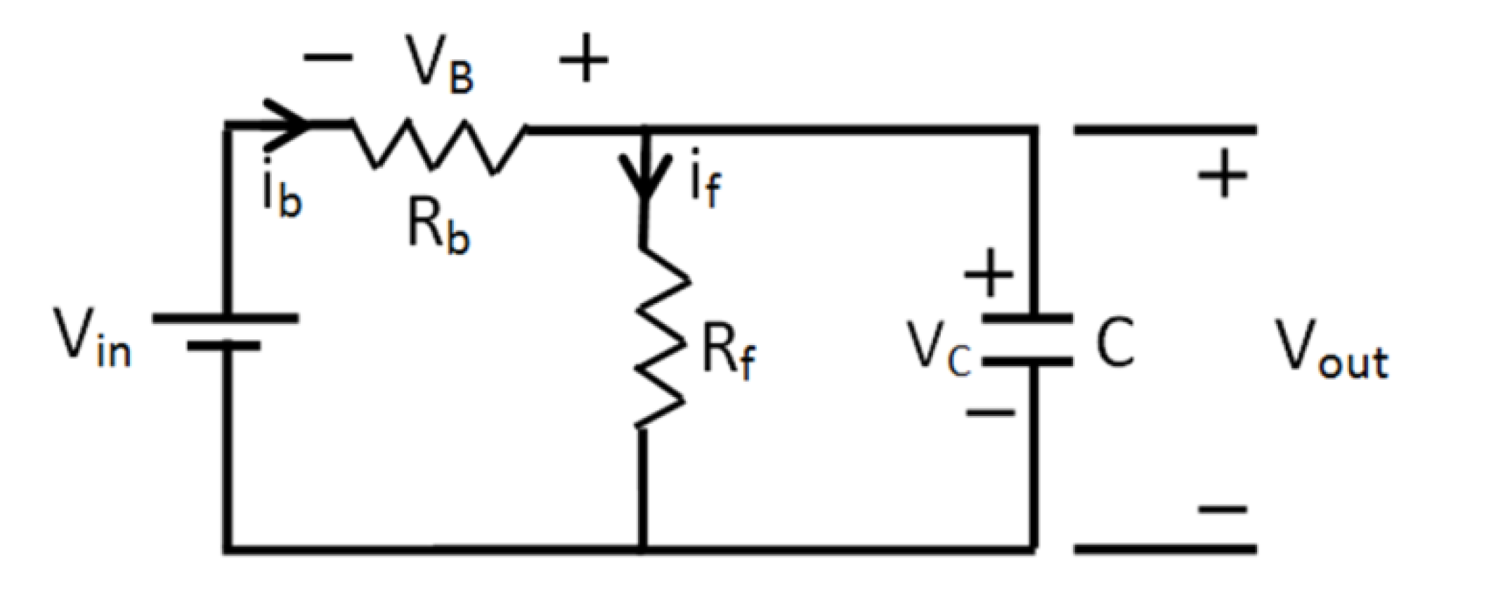
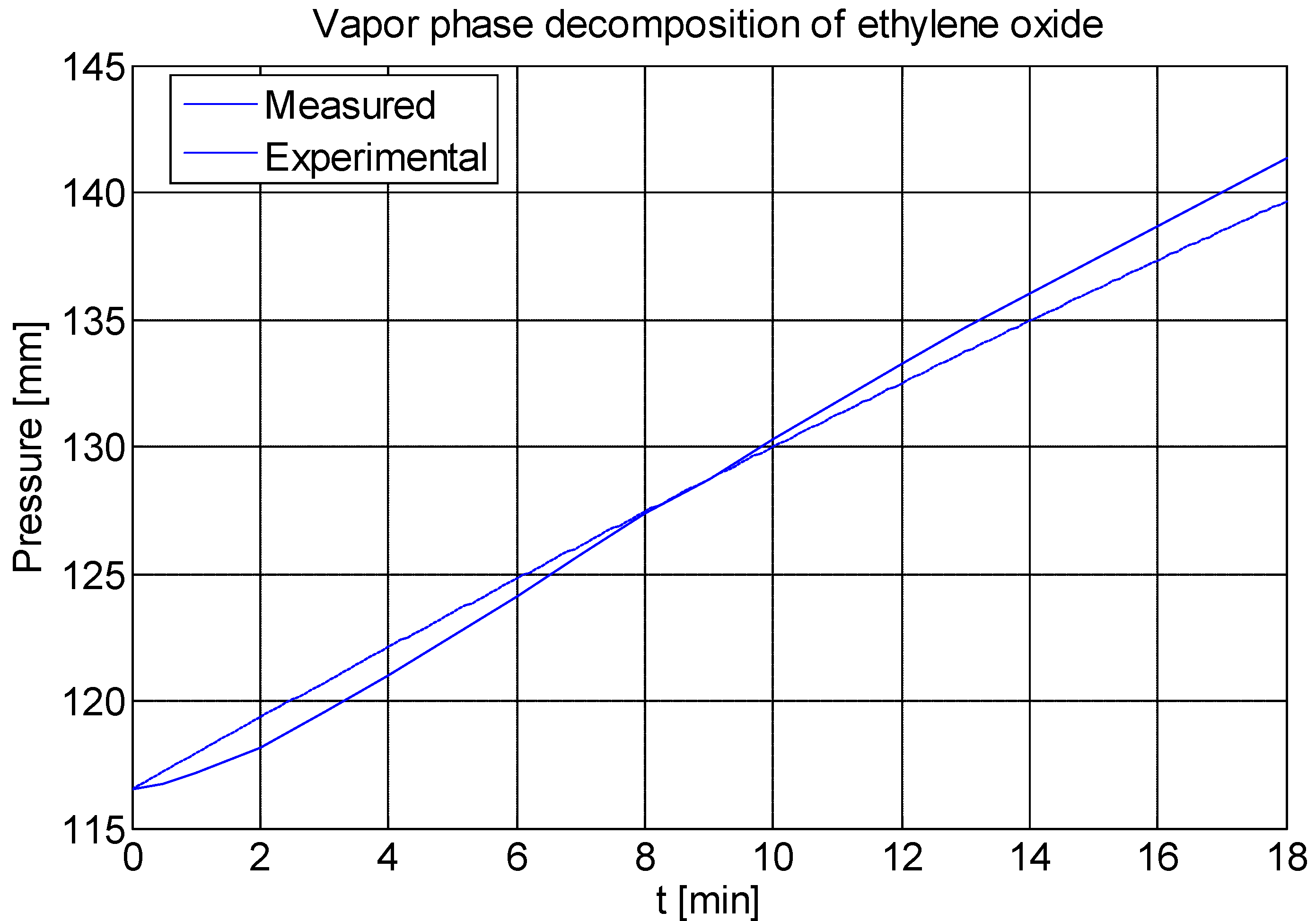
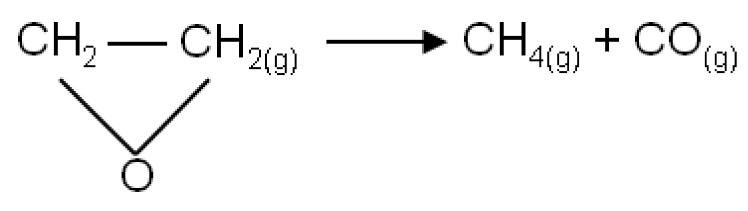
was adjusted in the electrical circuit in order to obtain compatibility with experimental reference data. The constant that gave good compatibility was k = 0.0123 [min−1], which is indeed the correct rate constant of this reaction. Figure 8 shows the compatibility between the experimental reference data and the measured analogous output (i.e., voltage) related to the adjusted rate constant. The experimental data and the measured voltage were drawn in solid and dashed lines, respectively.
Figure 8. Vapor phase decomposition of ethylene oxide. A comparison between experimental data and simulation results acquired using the analogous electrical model.
Processes 01 00012 g008

3.2. Opto-Chemical Analysis

The analogous electrical model for measuring and calculating the precise time behavior of concentration in general chemical reaction has been shown in Section 2 and Section 3.1. Nonetheless, the suggested model can be extended for investigation of optical and bio chemical processes.
The rate of the induced emission or absorption influenced by the power of the radiation10 can be described by:
Processes 01 00012 i023
where λm is the wavelength of the radiation, τsp is the spontaneous lift time of the level, g(υ − υo) is the chart of the atoms level spectral reaction, ρ(υ) is the spectral structure of the illuminating radiation having units of Processes 01 00012 i024
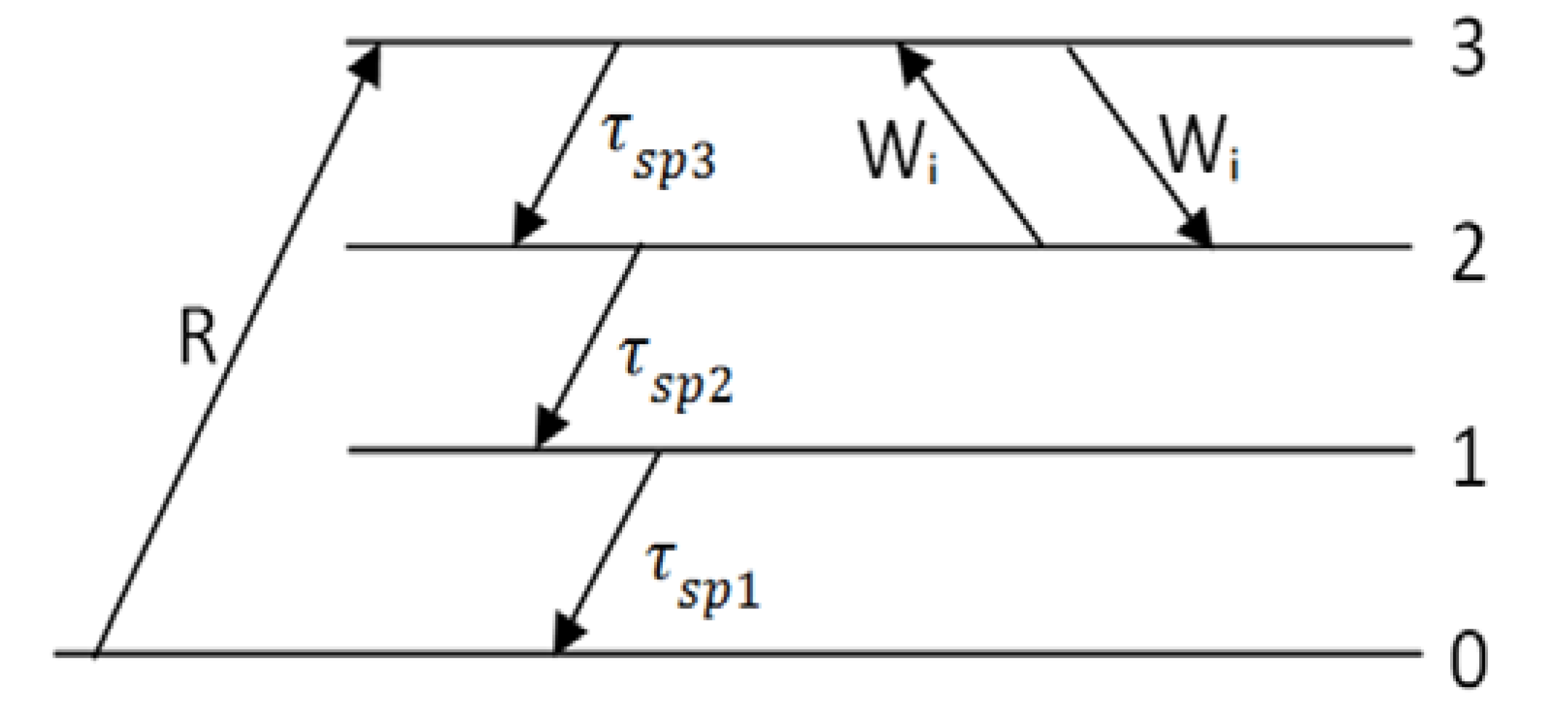
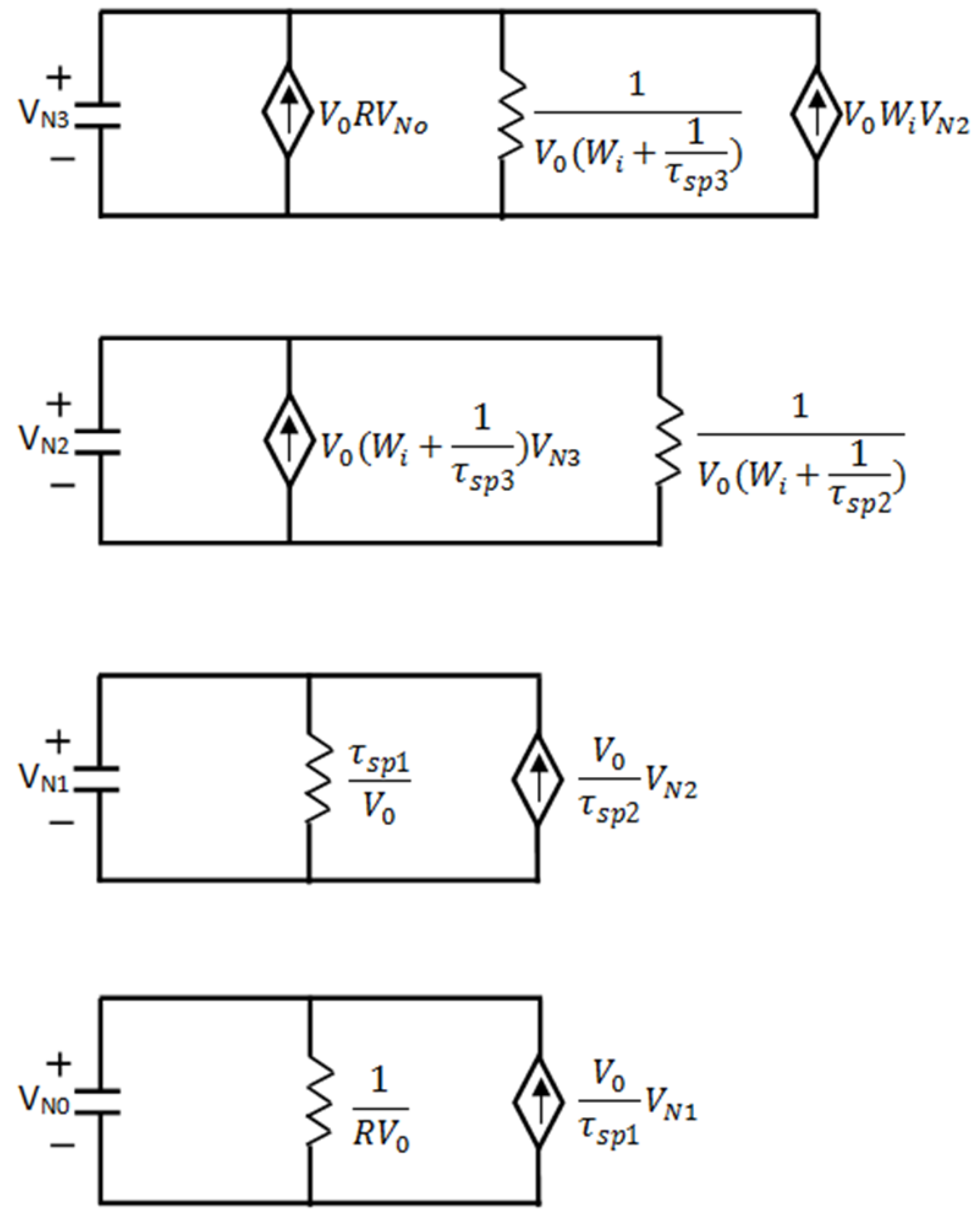
, υ is the radiation frequency and υo is the atom’s resonant frequency. h = 6.626 × 10⁻³⁴ [J·sec] is the Planck’s constant. The common case is related to a narrow band illumination described by:
ρ(υ′) = ρυ δ(υ′υ)
where δ(υ') is the delta function of Dirac. In this case the rate Wi will be:
Processes 01 00012 i025
In the investigated example, a pressure broadening is assumed and thus g(υ − υo) is:
Processes 01 00012 i026
where Processes 01 00012 i027 and Processes 01 00012 i028. a and M are the atom’s radius and mass, respectively, P is the pressure in the tube and T is the temperature. In the experimental simulation we assumed that the material is illuminated at a radiation frequency that is near the resonant frequency of the atom υo and thus:
Processes 01 00012 i029
This model is applied on a four level laser configuration as illustrated in Figure 9.
Figure 9. The energy model of a four level laser.
Processes 01 00012 g009
Where R is pumping rate of the laser. The material is illuminated with monochromatic radiation with frequency close to υ32 = υ3 − υ2 and thus the induced emission and absorption occurs between the second and the third energy levels. The rate equations9 are as follows:
Processes 01 00012 i030
Processes 01 00012 i031
Processes 01 00012 i032
Processes 01 00012 i033
where Ni and τspi are the concentration of the atoms and the relaxation time related to the spontaneous process at the i energy level, respectively. Another essential equation is related to the material conservation defined by:
N = N0 + N1 + N2 + N3
Figure 10 shows the analogous electrical circuit of a four level laser configuration.
Figure 10. The analogous electrical model of atoms concentrations at each one of the four levels of the laser.
Processes 01 00012 g010

3.3. Bio Chemical Applications

3.3.1. Bio Chemical Analysis of Kinetics of Cell’s Membrane

In this section, we analyzed the time behavior of concentrations flowing through a membrane. The definition of flux, J is:
Processes 01 00012 i034
where u is the mobility, C is the concentration, f is a force, I is the current, A is the membrane area and m is the mass of the material. We will investigate two types of forces, a force coming from electrical potential as well as a force coming from a chemical potential (diffusion). The force coming from electrical field acting on a single ion is [11,12]
Processes 01 00012 i035
Where Z is the valence of the material, F is Faraday’s constant, N0 is Avogadro constant and ψ is the electrical potential. The diffusivity is defined as:
Processes 01 00012 i036
where T is the temperature and R is the gas constant. Thus:
Processes 01 00012 i037
The flux coming from diffusion:
Processes 01 00012 i038
We will assume that the concentration of the material is changed linearly between the two sides of the membrane as illustrated in Figure 11, thus:
Processes 01 00012 i039
where Δx is the width of the membrane.
Figure 11. Schematic sketch of the concentration distribution assumption.
Processes 01 00012 g011
The analyzed case is a membrane separating between two cells, whereas each cell contains different concentrations of NaCl. We will denote the concentration of Na and Cl in the left cell as [Na+]1 and [Cl]1, respectively and [Na+]2 and [Cl]2 for the right side, respectively. In our system, we chose the interesting case where only the Na can penetrate the membrane and the Cl cannot. Due to the diffusion, atoms of Na will penetrate the membrane and electrical field will develop. Eventually this field will stop the diffusion potential and the membrane will be charged with electrical charge according to the law of Gauss. Thus, producing an electrical field of:
Processes 01 00012 i040
where σ is the surface charge, ε is the dielectric constant of the membrane and ψ is the electric potential.
Processes 01 00012 i041
V0 is the volume of the cell, A is the cross section area of the membrane and e is the electron charge. The mass as a function of the concentration is:
m = CV0Mw
where Mw is the molar weight of the material. The equation for the total flux is:
Processes 01 00012 i042
With our assumptions one may write the following set of equations:
Processes 01 00012 i043
Processes 01 00012 i044
whereas K1 and K2 can be defined as:
Processes 01 00012 i045
Processes 01 00012 i046
The material conservations law is:
Processes 01 00012 i047
As shown before, the flux coming from the electrical field is proportional to the multiplication between the electrical field and the concentration. The concentration of [Na+]2 was taken since the right side of the membrane will be occupied only by Na+ and the left side by Cl. No Na+ will be near the membrane’s left side due to the rejection of the electrical field. Because of this reason, Cl appears at the membrane’s right side. Equations (47) and (48) are being easily modified according to the analogous electrical model. Thus, the analogous electrical circuits can be illustrated according to Figure 12. All the capacitors capacity is Vo.
Figure 12. The analogous electrical circuits of concentrations [Na+]1 and [Na+]2 related to the flow through cell’s membrane.
Processes 01 00012 g012
If the membrane is made out of metal, the equations become much simpler, since no electric potential exists between the two cells:
Processes 01 00012 i048
Processes 01 00012 i049
The conservation of material:
Processes 01 00012 i050
The analogous circuit for this case is illustrated in Figure 13.
Figure 13. The analogous electrical circuit of concentrations [Na+]1 and [Na+]2 that are related to a flow through a metallic membrane.
Processes 01 00012 g013

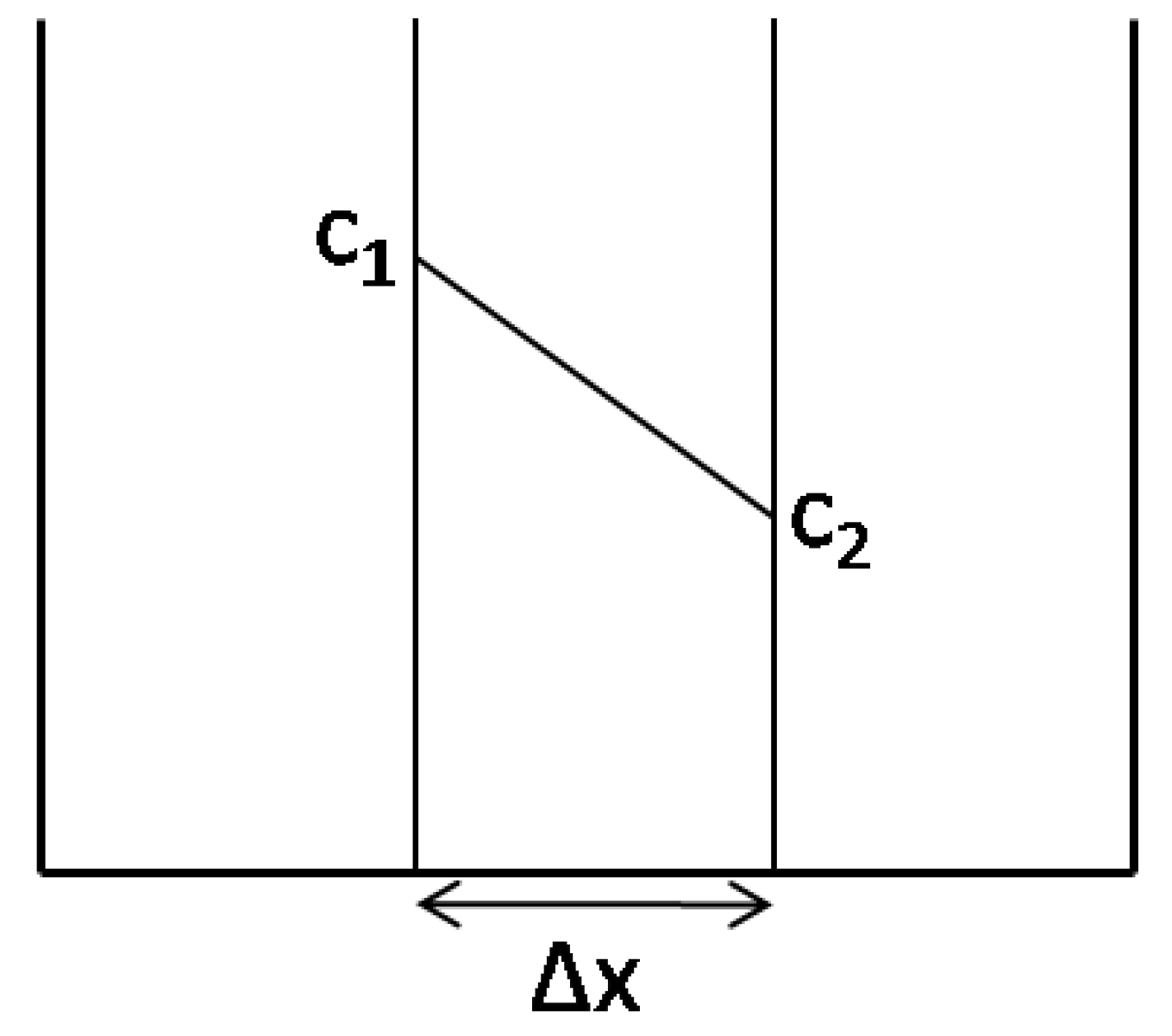
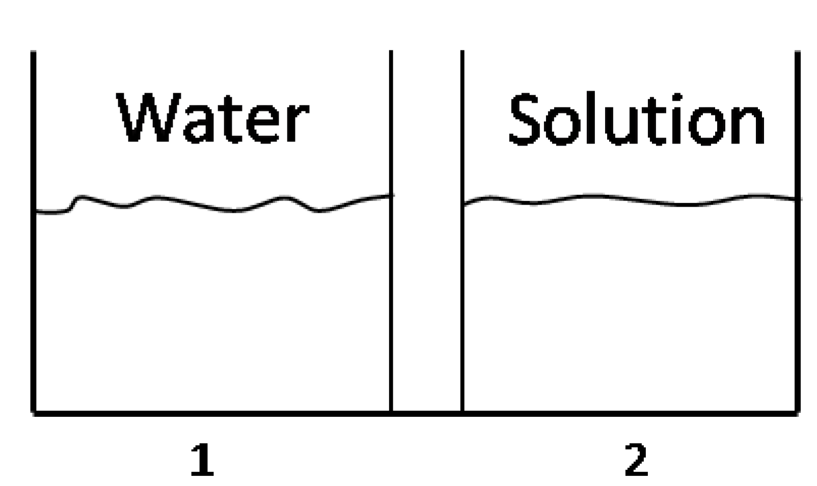
3.3.2. Osmosis Kinetics

In this case, we investigate an osmosis system in which the intermediate membrane is penetrable only for water. The schematic sketch of the system is illustrated in Figure 14.
Figure 14. Schematic sketch of the osmosis system. The intermediate membrane is penetrable only for water.
Processes 01 00012 g014
In the left cell, there is only water while on the right cell there is water and dissolved solid. In this system the flux is [11,12].
Processes 01 00012 i051
where μ is the chemical potential (diffusion), P is the pressure, n2w is the number of water moles in cell number two, V2 is the volume of the second cell and ρw is the specific weight of water. We will assume that between the two cells there is a linear change of the chemical potential and the pressure. Thus:
Processes 01 00012 i052
Processes 01 00012 i053
where, Δx is the width of the membrane. The chemical potential can be described using a known relation of:
μ = μs + RTlnχw
where χw is the molar fraction of water defined by:
Processes 01 00012 i054
nw is the number of moles of water and ns is the number of moles of the dissolved solid. Thus:
Processes 01 00012 i055
Since in the left cell (i.e., cell number 1) there is only water Processes 01 00012 i056. Thus, Using
Processes 01 00012 i057
One may write
μ2μ1 = RTln(1 − X2s) ≈ RT X2s
Now, we shall explore the pressure difference between the two cells:
P2P1 = g(ρ2h2ρ1h1)
where h1, h2 are the heights of the water level in each cell and ρ is the specific weight. Approximately, one may write:
ρ2ρ1 = ρw
where ρw is the specific weight of water. Since:
Processes 01 00012 i058
while Processes 01 00012 i059 
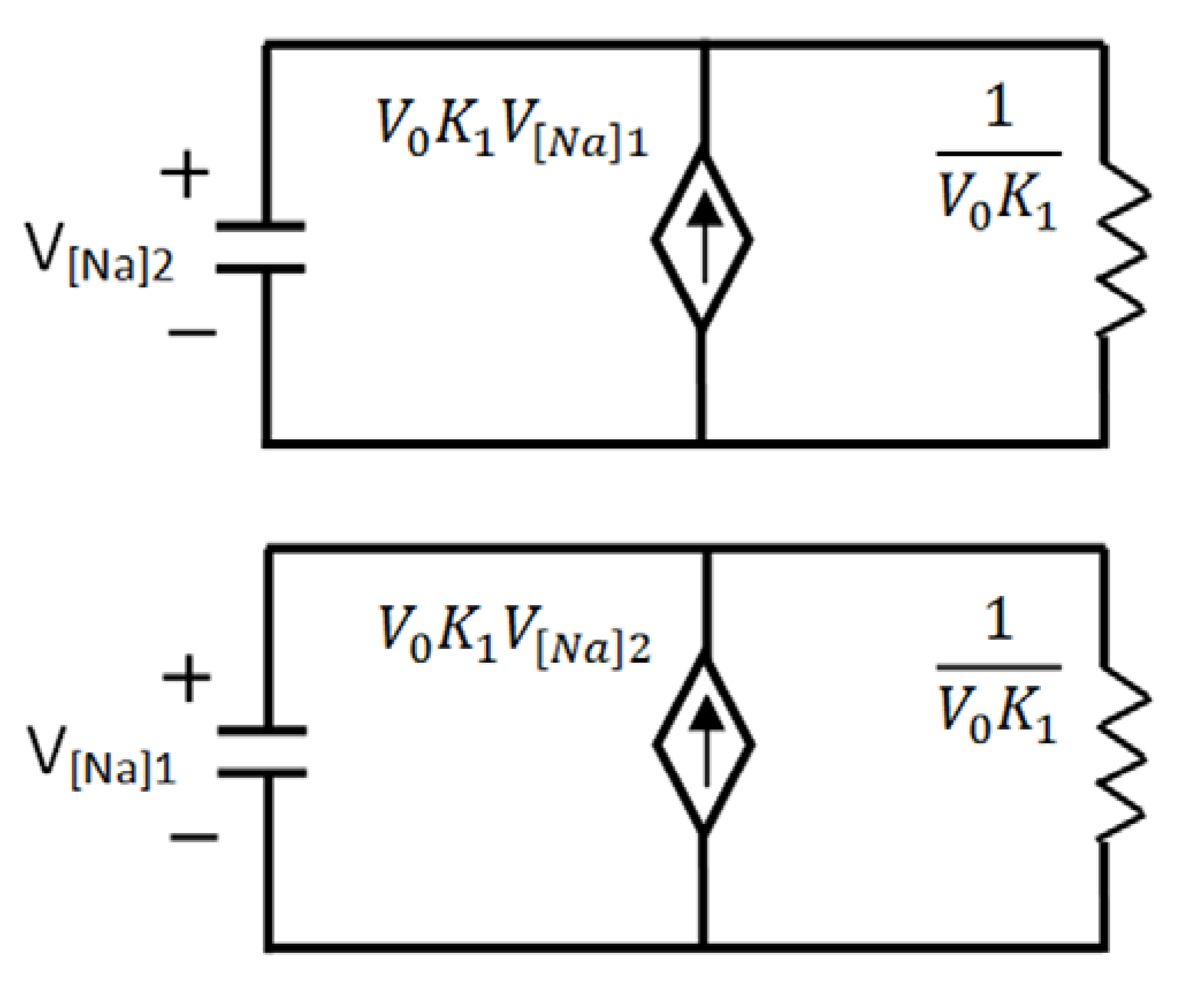
is the molar weight of water and V is the volume. Specifically in our case V1, V2 denote the volumes of the left and right cells, respectively. Using
Processes 01 00012 i060
The obtained heights are thus:
Processes 01 00012 i061
Processes 01 00012 i062
where S is the surface area of water in the cell. We will assume that the cell has the same diameter and thus, S1 = S2 = S. Approximately:
Processes 01 00012 i063
And the flux equations are:
Processes 01 00012 i064
Processes 01 00012 i065
Processes 01 00012 i066 
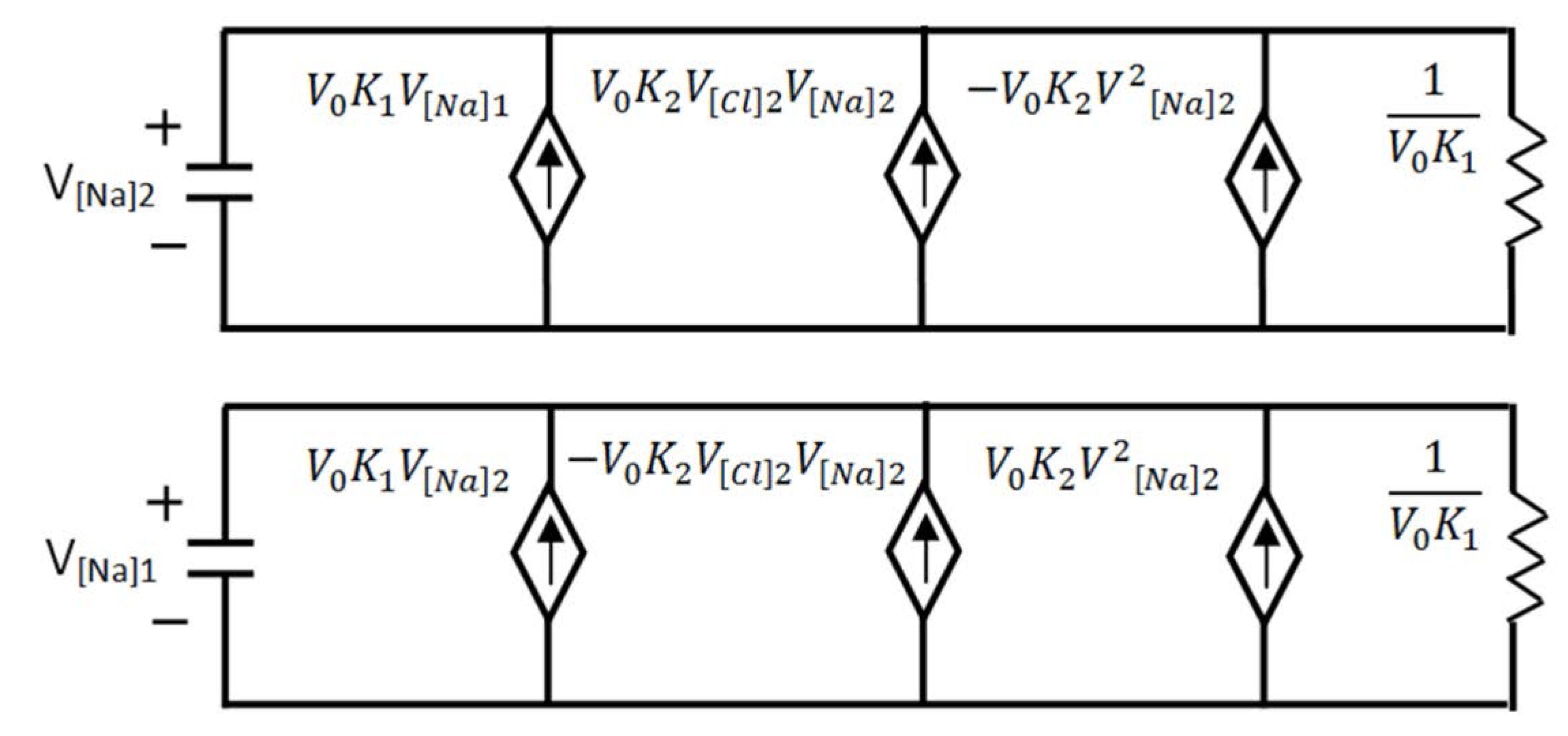
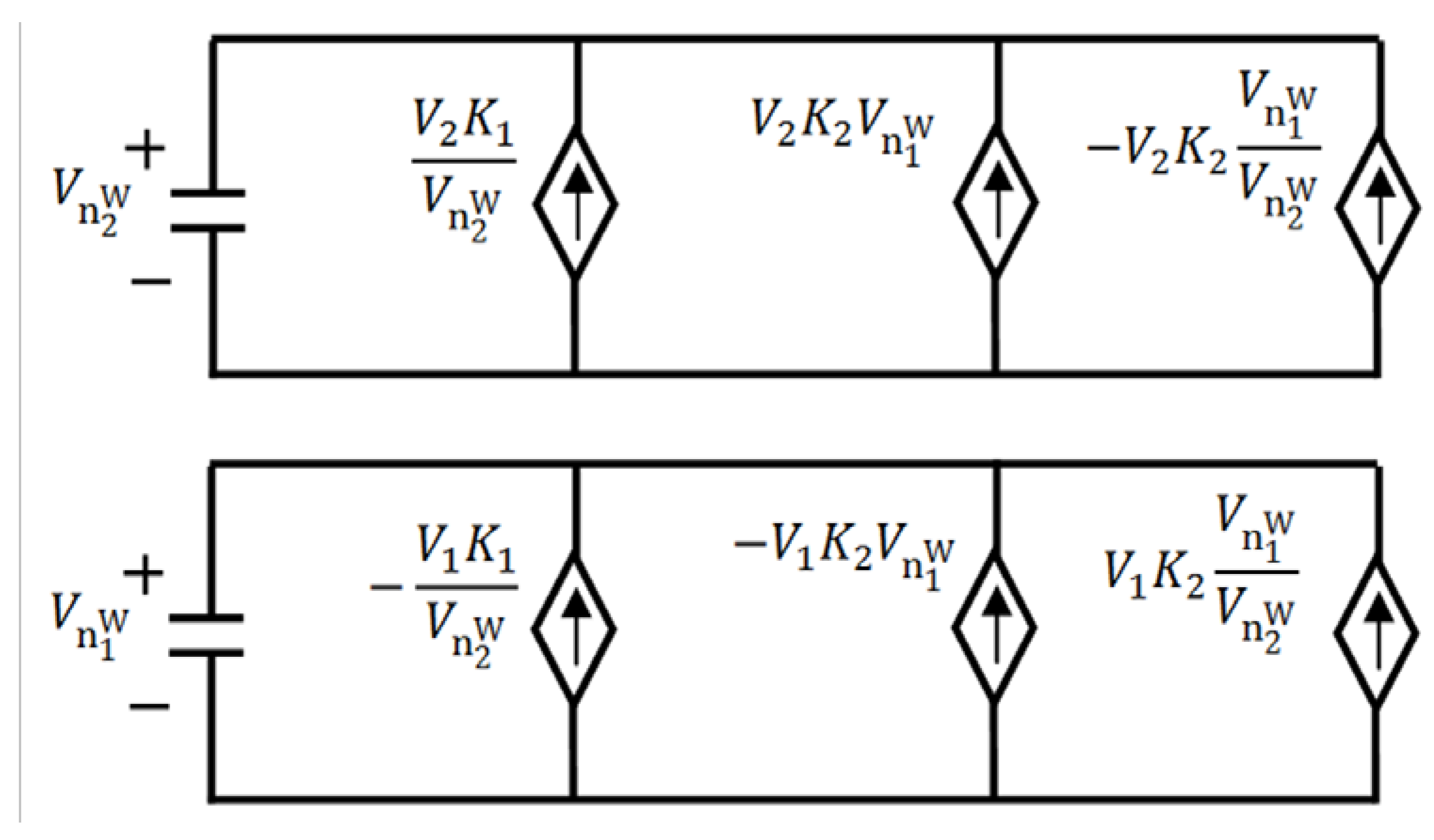
is constant for the process and thus the equations may rewritten as:
Processes 01 00012 i067
Processes 01 00012 i068
where,
Processes 01 00012 i069
Processes 01 00012 i070
Those equations can convert into the electrical circuits according to the aforementioned analogous electrical model. The equivalent circuits are illustrated in Figure 15.
Figure 15. The analogous electrical circuit of number of moles Processes 01 00012 i071 and Processes 01 00012 i072 that are related to the osmosis system analysis.
Processes 01 00012 g015
Note that the capacitor whose voltage is analogous to the concentration Processes 01 00012 i072 has the capacity of V2, while the capacitor whose voltage is analogous to the concentration Processes 01 00012 i071 has the capacity of V1.

4. Conclusions

In this paper, we have presented the analogous electrical model for analyzing and determining the time dependence of variety of applications in the fields of chemistry, biology, bio-chemistry and optics. The main advantage of this analogous model is that it makes easier to investigate chemical or physical processes whose parameters are unknown, by applying the proper analogous electrical circuit. The latter allows one to study the output of this circuit by changing the value of one of its components (i.e., a resistor). In addition, the analogous electrical system can be synthesized with the help of several software packages, which were originally written for electrical engineering applications. Our duality model can open a window for such design techniques in many fields instead of dealing directly with differential equations. The output voltage (which is analogous to the analyzed parameter) will be obtained as fast as the speed of light. The analogous model for the chemical reactions, opto-chemical analysis and biochemical applications were demonstrated and discussed.

References

  1. Bamford, C.H.; Tipper, C.F.H. Comprehensive Chemical Kinetics; Elsevier: New York, NY, USA, 1969; Volume 2. [Google Scholar]
  2. Heckert, W.; Mack, E. The Thermal decomposition of gaseous ethylene oxide. J. Am. Chem. Soc. 1929, 51, 2706–2717. [Google Scholar] [CrossRef]
  3. Palani, S. Control. System Engineering; Tata McGraw-Hill: Noida, India, 2010. [Google Scholar]
  4. Kamlesh, M.T.; Wood, J.H.; Mikulecky, D.C. Dynamic simulation of pharmacokinetic systems using the electrical circuit analysis program SPICE2. Comput. Progr. Biomed. 1982, 15, 61–72. [Google Scholar] [CrossRef]
  5. D’Azzo, J.J.; Houpis, C.H.; Sheldon, S.N. Linear Control. System Analysis and Design; CRC: New York, NY, USA, 2003. [Google Scholar]
  6. Wang, C.; Nehrir, M.H.; Shaw, S.R. Dynamic models and model validation for PEM fuel cells using electrical circuits, Energy Conversion. IEEE Trans. 2005, 20, 442–451. [Google Scholar]
  7. Fletcher, S. An electrical model circuit that reproduces the behaviour of conducting polymer electrodes in electrolyte solutions. J. Electroanal. Chem. 1992, 337, 127–145. [Google Scholar]
  8. User Manual for PSpice software. Available online: http://www.cadence.com/products/orcad/pspice_simulation/pages/default.aspx (accessed on 20 August 2012).
  9. Siegman, A.E. Lasers; University Science Books: Sausalito, CA, USA, 1986. [Google Scholar]
  10. Stryer, L. Biochemistry, 4th ed; W.H. Freeman and Company: New York, NY, USA, 1995. [Google Scholar]
  11. Sheeler, P.; Bianchi, D.E. Cell Biology; John Wiley & Sons, Inc: New York, NY, USA, 1987. [Google Scholar]
  12. Alberty, R.A.; Silbey, J.R. Physical Chemistry; John Wiley & Sons, Inc.: New York, NY, USA, 1992. [Google Scholar]

