
Innovative Solutions to the Fractional Diffusion Equation Using the Elzaki Transform

 ,
,  , and
, and 
Abstract
:1. Introduction
2. Basic Definitions
Transformation of Fractional Derivatives via the Elzaki Transform
3. Variational Iteration Transform Method (VITM)
4. Application
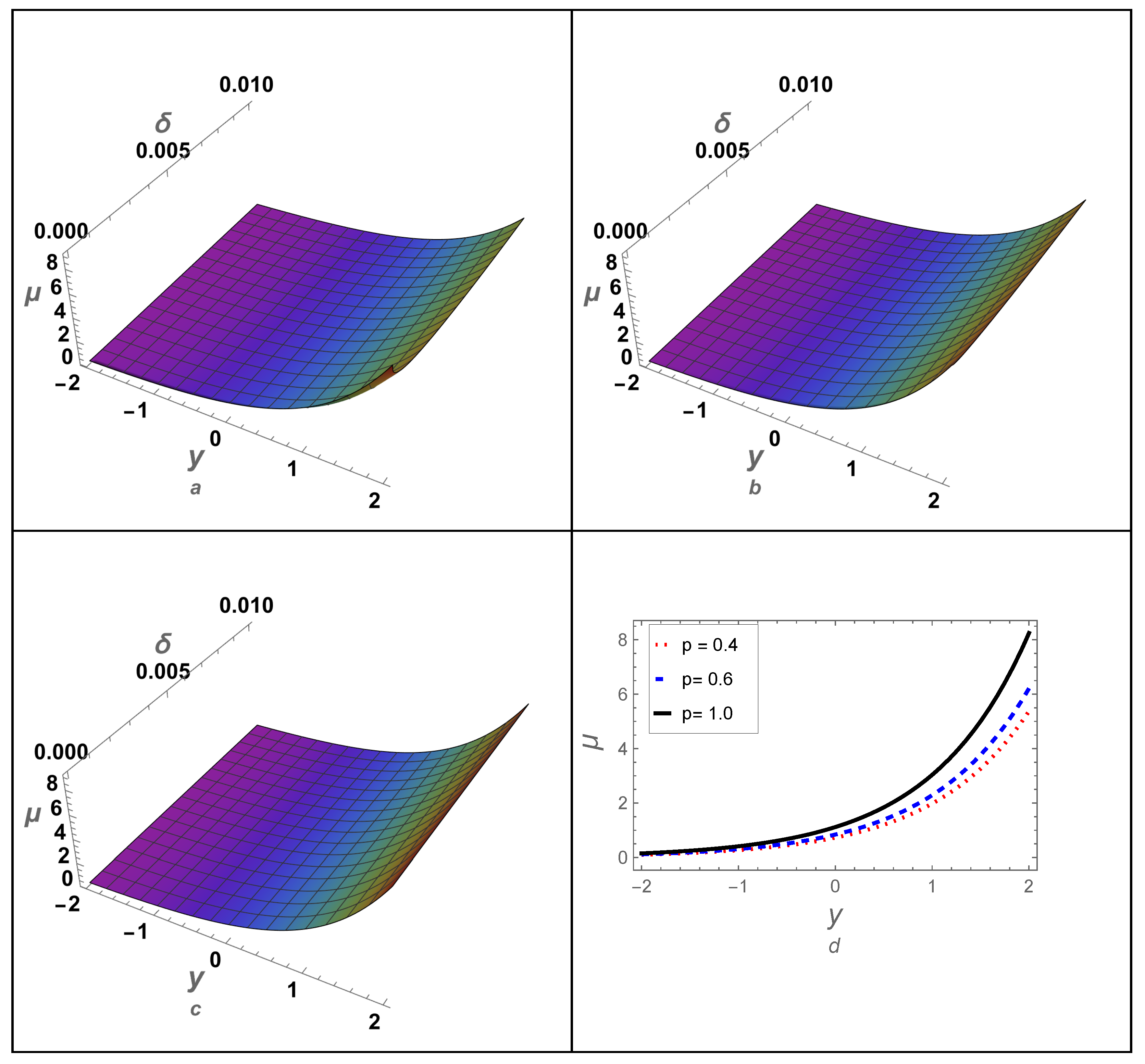
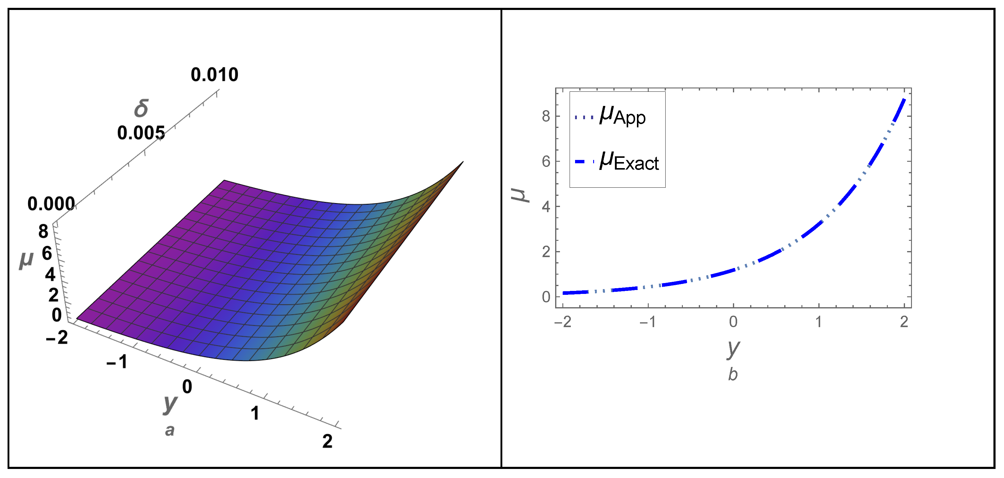
4.1. Example-(I)
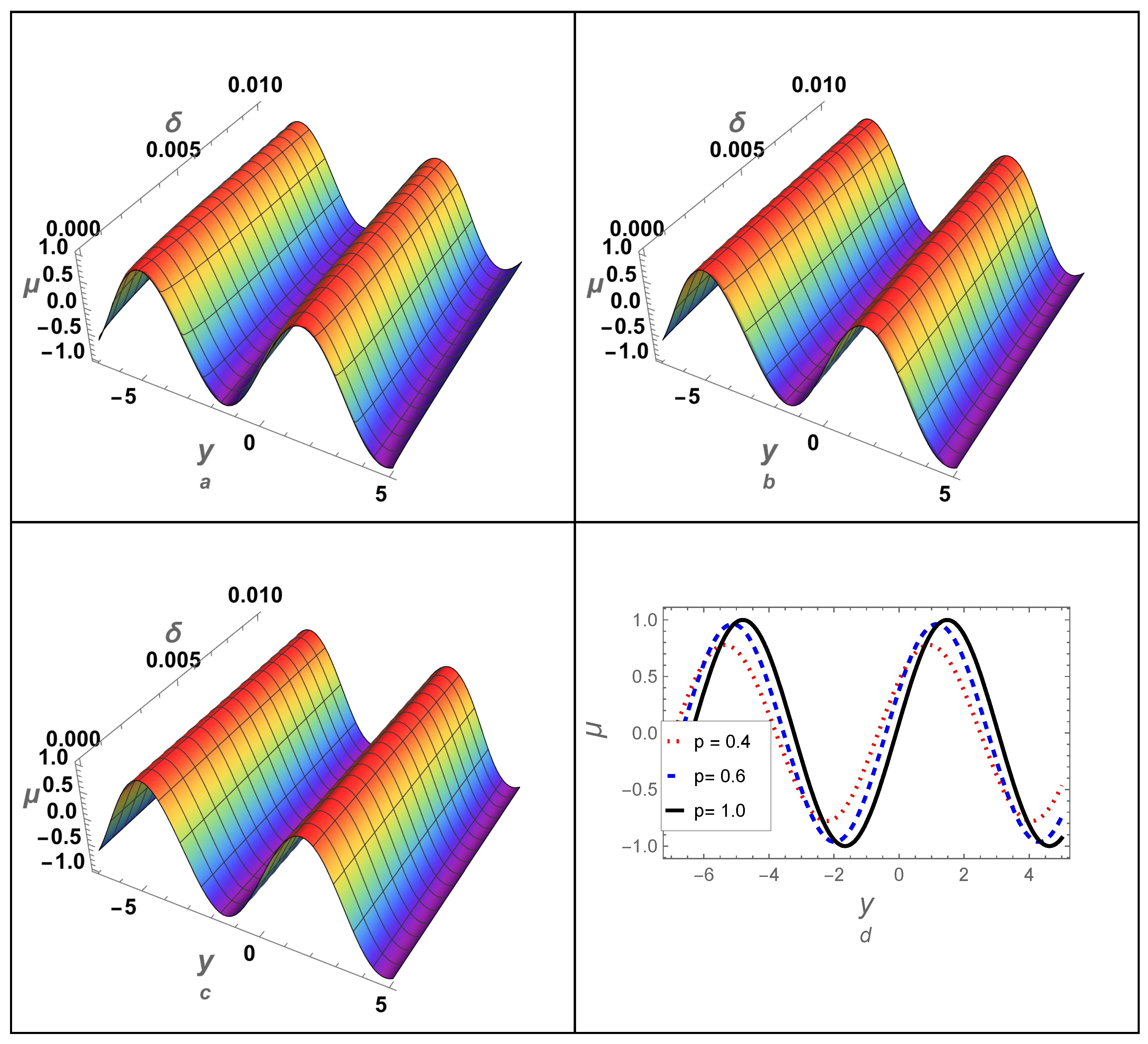
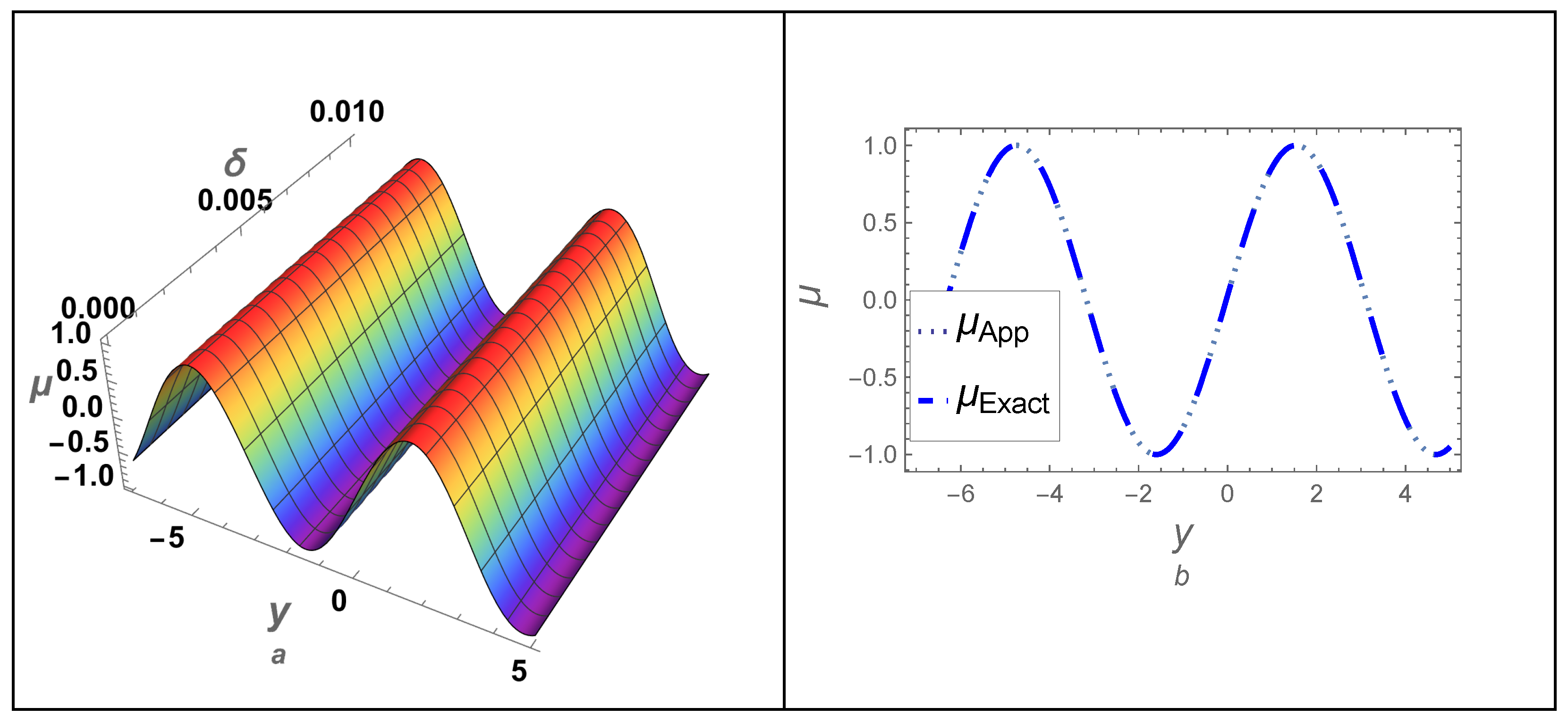
4.2. Example-(II)
5. Conclusions
Author Contributions
Funding
Data Availability Statement
Acknowledgments
Conflicts of Interest
References
- Du, M.; Wang, Z.; Hu, H. Measuring memory with the order of fractional derivative. Sci. Rep. 2013, 3, 3431. [Google Scholar] [CrossRef] [PubMed]
- Caputo, M. Elasticita Dissipazione (Elasticity and Anelastic Dissipation); Zanichelli: Bologna, Italy, 1969; Volume 4, p. 98. [Google Scholar]
- Miller, K.S.; Ross, B. An Introduction to the Fractional Calculus and Fractional Differential Equations; John Wiley & Sons: New York, NY, USA, 1993. [Google Scholar]
- Podlubny, I. Fractional Differential Equations: An Introduction to Fractional Derivatives, Fractional Differential Equations, to Methods of Their Solution and Some of Their Applications; Elsevier: Amsterdam, The Netherlands, 1998. [Google Scholar]
- Scalas, E.; Gorenflo, R.; Mainardi, F. Fractional calculus and continuous-time finance. Phys. A Stat. Mech. Its Appl. 2000, 284, 376–384. [Google Scholar] [CrossRef]
- West, B.J.; Turalska, M.; Grigolini, P. Fractional calculus ties the microscopic and macroscopic scales of complex network dynamics. New J. Phys. 2015, 17, 045009. [Google Scholar] [CrossRef]
- Tarasov, V.E. Fractional vector calculus and fractional Maxwell’s equations. Ann. Phys. 2008, 323, 2756–2778. [Google Scholar] [CrossRef]
- Tao, H.; Anjum, N.; Yang, Y.J. The Aboodh transformation-based homotopy perturbation method: New hope for fractional calculus. Front. Phys. 2023, 11, 1168795. [Google Scholar] [CrossRef]
- Ain, Q.T.; Anjum, N.; Din, A.; Zeb, A.; Djilali, S.; Khan, Z.A. On the analysis of Caputo fractional order dynamics of Middle East Lungs Coronavirus (MERS-CoV) model. Alex. Eng. J. 2022, 61, 5123–5131. [Google Scholar] [CrossRef]
- Zhang, Y.; Anjum, N.; Tian, D.; Alsolami, A.A. Fast And Accurate Population Forecasting with Two-Scale Fractal Population Dynamics and Its Application to Population Economics. Fractals 2024, 32, 2450082. [Google Scholar] [CrossRef]
- Anjum, N.; Ain, Q.T.; Li, X.X. Two-scale mathematical model for tsunami wave. GEM-Int. J. Geomath. 2021, 12, 10. [Google Scholar] [CrossRef]
- Alhejaili, W.; Az-Zo’bi, E.; Shah, R.; El-Tantawy, S.A. On the analytical soliton approximations to fractional forced Korteweg-de Vries equation arising in fluids and Plasmas using two novel techniques. Commun. Theor. Phys. 2024, 76, 085001. [Google Scholar] [CrossRef]
- Noor, S.; Albalawi, W.; Shah, R.; Al-Sawalha, M.M.; Sherif, M.E.; Ismaeel, S.M.E.; El-Tantawy, S.A. On the approximations to fractional nonlinear damped Burger’s-type equations that arise in fluids and plasmas using Aboodh residual power series and Aboodh transform iteration methods. Front. Phys. 2024, 12, 1374481. [Google Scholar] [CrossRef]
- Kilbas, A.A.; Srivastava, H.M.; Trujillo, J.J. Theory and Applications of Fractional Differential Equations; Elsevier: Amsterdam, The Netherlands, 2006; Volume 204. [Google Scholar]
- Noor, S.; Albalawi, W.; Shah, R.; Shafee, A.; Sherif, M.E.; Ismaeel, S.M.E.; El-Tantawy, S.A. A comparative analytical investigation for some linear and nonlinear time-fractional partial differential equations in the framework of the Aboodh transformation. Front. Phys. 2024, 12, 1374049. [Google Scholar] [CrossRef]
- Bekir, A.; Aksoy, E.; Cevikel, A.C. Exact solutions of nonlinear time fractional partial differential equations by sub-equation method. Math. Methods Appl. Sci. 2015, 38, 2779–2784. [Google Scholar] [CrossRef]
- Khuri, S.A.; Sayfy, A. A Laplace variational iteration strategy for the solution of differential equations. Appl. Math. Lett. 2012, 25, 2298–2305. [Google Scholar] [CrossRef]
- Nadeem, M.; Li, F.; Ahmad, H. Modified Laplace variational iteration method for solving fourth-order parabolic partial differential equation with variable coefficients. Comput. Math. Appl. 2019, 78, 2052–2062. [Google Scholar] [CrossRef]
- Nadeem, M.; He, J.H.; Sedighi, H.M. Numerical analysis of multi-dimensional time-fractional diffusion problems under the Atangana-Baleanu Caputo derivative. Math. Biosci. Eng. 2023, 20, 8190–8207. [Google Scholar] [CrossRef]
- Anjum, N.; He, J.H. Laplace transform: Making the variational iteration method easier. Appl. Math. Lett. 2019, 92, 134–138. [Google Scholar] [CrossRef]
- Ul Rahman, J.; Lu, D.; Suleman, M.; He, J.H.; Ramzan, M. He-Elzaki method for spatial diffusion of biological population. Fractals 2019, 27, 1950069. [Google Scholar] [CrossRef]
- Ji-Huan, H.E.; Anjum, N.; Chun-Hui, H.E.; Alsolami, A.A. Beyond Laplace and Fourier transforms Challenges and Future Prospects. Therm. Sci. 2023, 27, 5075–5089. [Google Scholar]
- El-Tantawy, S.A.; Matoog, R.T.; Shah, R.; Alrowaily, A.W.; Ismaeel, S.M.E. On the shock wave approximation to fractional generalized Burger–Fisher equations using the residual power series transform method. Phys. Fluids 2024, 36, 023105. [Google Scholar] [CrossRef]
- Gorenflo, R.; Mainardi, F. Some recent advances in theory and simulation of fractional diffusion processes. J. Comput. Appl. Math. 2009, 229, 400–415. [Google Scholar] [CrossRef]
- Jiang, X.; Xu, M.; Qi, H. The fractional diffusion model with an absorption term and modified Fick’s law for non-local transport processes. Nonlinear Anal. Real World Appl. 2010, 11, 262–269. [Google Scholar] [CrossRef]
- Sokolov, I.M.; Chechkin, A.V.; Klafter, J. Fractional diffusion equation for a power-law-truncated Levy process. Phys. A Stat. Mech. Its Appl. 2004, 336, 245–251. [Google Scholar] [CrossRef]
- Meerschaert, M.M.; Zhang, Y.; Baeumer, B. Particle tracking for fractional diffusion with two time scales. Comput. Math. Appl. 2010, 59, 1078–1086. [Google Scholar] [CrossRef]
- Goychuk, I.; Hanggi, P. Fractional diffusion modeling of ion channel gating. Phys. Rev. E 2004, 70, 051915. [Google Scholar] [CrossRef] [PubMed]
- Berestycki, H.; Roquejoffre, J.M.; Rossi, L. The periodic patch model for population dynamics with fractional diffusion. Discret. Contin. Dyn. Syst. Ser. S 2011, 4, 1–13. [Google Scholar] [CrossRef]
- Cartea, A.; del-Castillo-Negrete, D. Fractional diffusion models of option prices in markets with jumps. Phys. A Stat. Mech. Its Appl. 2007, 374, 749–763. [Google Scholar] [CrossRef]
- Marom, O.; Momoniat, E. A comparison of numerical solutions of fractional diffusion models in finance. Nonlinear Anal. Real World Appl. 2009, 10, 3435–3442. [Google Scholar] [CrossRef]
- Elzaki, T.M. The new integral transform Elzaki transform. Glob. J. Pure Appl. Math. 2011, 7, 57–64. [Google Scholar]
- Elzaki, T.M. Application of new transform “Elzaki transform” to partial differential equations. Glob. J. Pure Appl. Math. 2011, 7, 65–70. [Google Scholar]
- Elzaki, T.M.; Ezaki, S.M. On the Elzaki transform and ordinary differential equation with variable coefficients. Adv. Theor. Appl. Math. 2011, 6, 41–46. [Google Scholar]
- Elzaki, T.M. Applications of New Transform “Elzaki Transform” to Mechanics, Electrical Circuits and Beams Problems; Research India Publications: Delhi, India, 2012; Volume 4. [Google Scholar]
- El-Tantawy, S.A.; Wazwaz, A.-M. Anatomy of modified Korteweg–de Vries equation for studying the modulated envelope structures in non-Maxwellian dusty plasmas: Freak waves and dark soliton collisions. Phys. Plasmas 2018, 25, 092105. [Google Scholar] [CrossRef]
- El-Tantawy, S.A.; Shan, S.A.; Mustafa, N.; Alshehri, M.H.; Duraihem, F.Z.; Bin Turki, N. Homotopy perturbation and Adomian decomposition methods for modeling the nonplanar structures in a bi-ion ionospheric superthermal plasma. Eur. Phys. J. Plus 2021, 136, 561. [Google Scholar] [CrossRef]
- Aljahdaly, N.; El-Tantawy, S.A.; Ashi, H.; Wazwaz, A.-M. Exponential time differencing scheme for Modeling the dissipative Kawahara solitons in a two-electrons collisional plasma. Rom. Rep. Phys. 2022, 74, 109. [Google Scholar]
- El-Tantawy, S.A.; Wazwaz, A.-M.; Ali Shan, S. On the nonlinear dynamics of breathers waves in electronegative plasmas with Maxwellian negative ions. Phys. Plasmas 2017, 24, 022105. [Google Scholar] [CrossRef]
- El-Tantawy, S.A.; Alharbey, R.A.; Salas, A.H. Novel approximate analytical and numerical cylindrical rogue wave and breathers solutions: An application to electronegative plasma. Chaos Solitons Fractals 2022, 155, 111776. [Google Scholar] [CrossRef]
- El-Tantawy, S.A.; Salas, A.H.; Alyousef, H.A.; Alharthi, M.R. Novel approximations to a nonplanar nonlinear Schrödinger equation and modeling nonplanar rogue waves/breathers in a complex plasma. Chaos Solitons Fractals 2022, 1635, 112612. [Google Scholar] [CrossRef]
- Elzaki, T.M.; Elzaki, S.M.; Elnour, E.A. On the New Integral Transform “ELzaki Transform” Fundamental Properties Investigations and Applications. Glob. J. Math. Sci. 2012, 4, 1–13. [Google Scholar]
- Elzaki, T.M.; Elzaki, S.M. On the Connections between Laplace and ELzaki Transforms. Adv. Theor. Appl. Math. 2014, 6, 1–10. [Google Scholar]
- Neamaty, A.; Agheli, B.; Darzi, R. New Integral Transform for Solving Nonlinear Partial Di erential Equations of fractional order. Theory Approx. Appl. 2016, 10, 69–86. [Google Scholar]
- Elzaki, T.M.; Kim, H. The solution of radial diffusivity and shock wave equations by Elzaki variational iteration method. Int. J. Math. Anal. 2015, 9, 1065–1071. [Google Scholar] [CrossRef]
- He, J.H. A variational iteration approach to nonlinear problems and its applications. Mech. Appl. 1998, 20, 30–31. [Google Scholar]
- Noor, S.; Albalawi, W.; Shah, R.; Al-Sawalha, M.M.; Ismaeel, S.M.E. Mathematical frameworks for investigating fractional nonlinear coupled Korteweg-de Vries and Burger’s equations. Front. Phys. 2024, 12, 1374452. [Google Scholar] [CrossRef]
- Wang, K.L.; He, C.H. A remark on Wang’s fractal variational principle. Fractals 2019, 27, 1950134. [Google Scholar] [CrossRef]

| y | |||
|---|---|---|---|
| −0.5 | 0.738599 | 0.738599 | 1.4432899320127035 |
| −0.4 | 0.816278 | 0.816278 | 1.6653345369377348 |
| −0.3 | 0.902127 | 0.902127 | 1.887379141862766 |
| −0.2 | 0.997004 | 0.997004 | 1.9984014443252818 |
| −0.1 | 1.10186 | 1.10186 | 2.220446049250313 |
| 0. | 1.21774 | 1.21774 | 2.4424906541753444 |
| 0.1 | 1.34582 | 1.34582 | 2.6645352591003757 |
| 0.2 | 1.48736 | 1.48736 | 2.886579864025407 |
| 0.3 | 1.64378 | 1.64378 | 3.3306690738754696 |
| 0.4 | 1.81666 | 1.81666 | 3.774758283725532 |
| 0.5 | 2.00772 | 2.00772 | 3.9968028886505635 |
| y | |||||
|---|---|---|---|---|---|
| −0.5 | 0.738599 | 0.738602 | 0.738599 | 1.44329 | 3.31707 |
| −0.4 | 0.816278 | 0.816282 | 0.816278 | 1.66533 | 3.66593 |
| −0.3 | 0.902127 | 0.902131 | 0.902127 | 1.88738 | 4.05148 |
| −0.2 | 0.997004 | 0.997009 | 0.997004 | 1.9984 | 4.47758 |
| −0.1 | 1.10186 | 1.10187 | 1.10186 | 2.22045 | 4.94849 |
| 0. | 1.21774 | 1.21775 | 1.21774 | 2.44249 | 5.46893 |
| 0.1 | 1.34582 | 1.34582 | 1.34582 | 2.66454 | 6.0441 |
| 0.2 | 1.48736 | 1.48736 | 1.48736 | 2.88658 | 6.67976 |
| 0.3 | 1.64378 | 1.64379 | 1.64378 | 3.33067 | 7.38228 |
| 0.4 | 1.81666 | 1.81667 | 1.81666 | 3.77476 | 8.15868 |
| 0.5 | 2.00772 | 2.00773 | 2.00772 | 3.9968 | 9.01673 |
| y | |||
|---|---|---|---|
| −0.5 | −0.476791 | −0.476791 | 1.7763568394002505 |
| −0.4 | −0.386653 | −0.386653 | 1.8318679906315083 |
| −0.3 | −0.292653 | −0.292653 | 1.887379141862766 |
| −0.2 | −0.195728 | −0.195728 | 1.9984014443252818 |
| −0.1 | −0.096848 | −0.096848 | 2.0122792321330962 |
| 0. | 0.003 | 0.003 | 2.024855977333928 |
| 0.1 | 0.102818 | 0.102818 | 2.0261570199409107 |
| 0.2 | 0.201609 | 0.201609 | 1.9984014443252818 |
| 0.3 | 0.298385 | 0.298385 | 1.9984014443252818 |
| 0.4 | 0.39218 | 0.39218 | 1.887379141862766 |
| 0.5 | 0.482056 | 0.482056 | 1.7763568394002505 |
| y | |||||
|---|---|---|---|---|---|
| −0.5 | −0.476791 | −0.476788 | −0.476791 | 1.77636 | 2.13763 |
| −0.4 | −0.386653 | −0.386652 | −0.386653 | 1.83187 | 1.73163 |
| −0.3 | −0.292653 | −0.292652 | −0.292653 | 1.88738 | 1.30832 |
| −0.2 | −0.195728 | −0.195727 | −0.195728 | 1.9984 | 0.871945 |
| −0.1 | −0.096848 | −0.0968475 | −0.096848 | 2.01228 | 0.426855 |
| 0. | 0.003 | 0.00299997 | 0.003 | 2.02486 | 0.0225 |
| 0.1 | 0.102818 | 0.102818 | 0.102818 | 2.02616 | 0.47163 |
| 0.2 | 0.201609 | 0.201608 | 0.201609 | 1.9984 | 0.916048 |
| 0.3 | 0.298385 | 0.298384 | 0.298385 | 1.9984 | 1.35131 |
| 0.4 | 0.39218 | 0.392178 | 0.39218 | 1.88738 | 1.77308 |
| 0.5 | 0.482056 | 0.482054 | 0.482056 | 1.77636 | 2.17712 |
Disclaimer/Publisher’s Note: The statements, opinions and data contained in all publications are solely those of the individual author(s) and contributor(s) and not of MDPI and/or the editor(s). MDPI and/or the editor(s) disclaim responsibility for any injury to people or property resulting from any ideas, methods, instructions or products referred to in the content. |
© 2024 by the authors. Licensee MDPI, Basel, Switzerland. This article is an open access article distributed under the terms and conditions of the Creative Commons Attribution (CC BY) license (https://creativecommons.org/licenses/by/4.0/).
Share and Cite
Noor, S.; Alrowaily, A.W.; Alqudah, M.; Shah, R.; El-Tantawy, S.A. Innovative Solutions to the Fractional Diffusion Equation Using the Elzaki Transform. Math. Comput. Appl. 2024, 29, 75. https://doi.org/10.3390/mca29050075
Noor S, Alrowaily AW, Alqudah M, Shah R, El-Tantawy SA. Innovative Solutions to the Fractional Diffusion Equation Using the Elzaki Transform. Mathematical and Computational Applications. 2024; 29(5):75. https://doi.org/10.3390/mca29050075
Chicago/Turabian StyleNoor, Saima, Albandari W. Alrowaily, Mohammad Alqudah, Rasool Shah, and Samir A. El-Tantawy. 2024. "Innovative Solutions to the Fractional Diffusion Equation Using the Elzaki Transform" Mathematical and Computational Applications 29, no. 5: 75. https://doi.org/10.3390/mca29050075