Creating and Controlling Polarization Singularities in Plasmonic Fields

Abstract

Nanoscale light fields near nanoplasmonic objects can be highly structured and can contain highly-subwavelength features. Here, we present the results of our search for the simplest plasmonic system that contains, and can be used to control, the smallest such optical feature: an optical singularity. Specifically, we study the field around subwavelength holes in a metal film and look for polarization singularities. These can be circular (C)-points, at which the polarization is circular, or linear (L)-lines, where the polarization is linear. We find that, depending on the polarization of the incident light, two or three holes are sufficient to create a wealth of these singularities. Moreover, we find for the two-hole system that C-points are created in multiples of eight. This can be explained using symmetry arguments and conservation laws. We are able to predict where these singularities are created, their index and the topology of the field surrounding them. These results demonstrate the promise of this plasmonic platform as a tool for studying and controlling fundamental properties of light fields and may be important to applications where control over these properties is required at the nanoscale.

1. Introduction

Structured light fields, which have long been studied at everyday length scales [1,2,3,4,5,6], are increasingly being identified and studied at the nanoscale. That this transition occurs should not be too surprising, after all, at the nanoscale, we can control optical properties, such as the speed [7,8,9,10] and way [11,12,13] in which light propagates, simply by engineering the structural geometry. What is surprising is how long it has taken for this transition to occur. After all, studies of fine structure in light fields, such as optical singularities, first appeared almost 70 years ago [14,15,16].

Perhaps investigations into the fine structure of nanoscale light fields were delayed because, initially, researchers were more interested in the macroscopic optical properties of nanopatterned materials, rather than their microscopic field structure. Studies of photonic crystal waveguides, where the geometry of a periodic array of holes in a thin semi-conductor layer determines the properties of the optical modes, are a perfect example of this phenomenon. Such waveguides were extensively studied for the way in which they guide light, generating considerable excitement for their ability to both highly confine light and to slow it down [7,8]. Yet, this very same nanopatterning, which controls the flow of light, also imprints a fine structure onto their nanoscale light fields. It is only recently that researchers have begun looking into the structured light fields of photonic crystal waveguides [17] and, through an understanding of this structure, explaining the origins of the macroscopic behavior of the waveguide [18].

One exciting type of structure in light fields, which we will focus on in this work, is the optical singularity and, more specifically, the polarization singularity [3,4]; these are amongst the smallest optical entities: infinitesimally small points in space where an aspect of the polarization of light (such as its handedness or orientation) is undefined and whose surrounding light fields carry a topological index. The recent studies of nanoscale optical singularities have been into the near fields of either highly structured dielectrics, such as photonic crystal waveguides [17,19,20], or the more simple plasmonic systems, such as slits or holes in metal films [21,22]. The latter, in part due to the underlying simplicity of the plasmonic systems, have illuminated key aspects of nanoscale singular optics and, in general, of light-matter interactions on the nanoscale. For example, these studies predict the nanoscale spatial evolution of optical singularities in complex light fields [21] and even offer a glimpse as to how they can be controlled and manipulated through nanoscale geometry [22]. These studies suggest that simple plasmonic systems can be used as a platform to study properties of optical singularities, at the nanoscale.

In this article, we set out to find the simplest plasmonic system where optical singularities can be created and controlled in a robust fashion. We use rigorous electromagnetic theory to numerically model the scattering of surface waves from subwavelength holes in metal films. We find that scattering from two holes, which act as dipole sources of surface plasmon polaritons that predominantly radiate towards each other, is sufficient to create light field distributions that contain polarization singularities. If we rotate the polarization of the incident light such that the scattering of the holes is predominantly in the orthogonal to the line containing the holes, then we find that three holes are required to generate polarization singularities. Finally, as an example, we show how using this simple plasmonic platform, we can create and annihilate singularities simply by changing the hole spacing or the polarization of the excitation beam.

2. Polarization Singularities in Plasmonic Fields

Polarization singularities are, by definition, points where some aspect of the polarization of a light field is undefined. At the nanoscale, these singularities can often be found in highly structured fields that arise, for example, from the interference of the different Bloch harmonics that form the eigenmodes of a photonic crystal waveguide [17,20] or the interference of incident and scattered surface plasmon polaritons (SPPs) from a nanoscatterer, such as a subwavelength hole [22]. If, for example, there are points, typically a line, at which the polarization of light is linear, then the handedness of the polarization ellipse there is undefined. This is called an L-line singularity. Likewise, if at a point, the polarization ellipse is circular, then at that point, its orientation is undefined. This is known as a C-point singularity.

When hunting for optical singularities in structured light fields, it is often simpler to consider the polarization properties of the light field, rather than its amplitude. At any point in space, the polarization of a monochromatic light field on a plane (we will take the x-y plane) of two field components (here, $E_x$ and $E_y$) can be described by an ellipse, as shown in Figure 1a.

Figure 1. Plasmonic platform for the study of optical singularities. (a) The polarization ellipse, which can be used to describe the polarization of light in a plane. Here, the lengths of the short and long axes, u and v, are labeled, as is α, the angle that the long axis makes with the y-axis. (b) Sketch of a plasmonic system that we envision can be used to study optical singularities on the nanoscale. Multiple holes, each separated by Λ, are arranged in a line on an optically thick metallic film. Illumination from the bottom side, in this case at normal incidence with $\mathbf{H}$ oriented along y and $\mathbf{E}$ along x, excites dipoles in the holes (in this case, predominately $m_y$), which radiate surface plasmon polaritons (SPPs) on the top surface of the film. We look for singularities in the electric field distributions that result from the superposition of all f the SPP waves. (c) The same system as in (b), but with the incident illumination rotated by 90 degrees, resulting in an initial response of the holes that is dominated by $m_x$. In this case, the holes will predominately launch SPPs in the $\widehat{y}$ direction.

Figure 1. Plasmonic platform for the study of optical singularities. (a) The polarization ellipse, which can be used to describe the polarization of light in a plane. Here, the lengths of the short and long axes, u and v, are labeled, as is α, the angle that the long axis makes with the y-axis. (b) Sketch of a plasmonic system that we envision can be used to study optical singularities on the nanoscale. Multiple holes, each separated by Λ, are arranged in a line on an optically thick metallic film. Illumination from the bottom side, in this case at normal incidence with $\mathbf{H}$ oriented along y and $\mathbf{E}$ along x, excites dipoles in the holes (in this case, predominately $m_y$), which radiate surface plasmon polaritons (SPPs) on the top surface of the film. We look for singularities in the electric field distributions that result from the superposition of all f the SPP waves. (c) The same system as in (b), but with the incident illumination rotated by 90 degrees, resulting in an initial response of the holes that is dominated by $m_x$. In this case, the holes will predominately launch SPPs in the $\widehat{y}$ direction.

This ellipse can be parameterized by ε and α, where:

$$\begin{array}{ccc}\hfill \epsilon \left(r\right)& =& tan\left\{{sin}^{-1}\left[sin\left(2\psi \left(r\right)\right)sin\left(\delta \left(r\right)\right)\right]/2\right\}\hfill \end{array}$$

(1)

$$\begin{array}{ccc}\hfill \alpha \left(r\right)& =& \left\{{tan}^{-1}\left[tan\left(2\psi \left(r\right)\right)cos\left(\delta \left(r\right)\right)\right]/2\right\}\hfill \end{array}$$

(2)

Here, $\psi \left(r\right)={tan}^{-1}\left[A_x\left(r\right)/A_y\left(r\right)\right]$ and $\delta \left(r\right)={\delta }_x\left(r\right)-{\delta }_y\left(r\right)$ are the ratio and difference of the field amplitudes and phases, respectively.

The ellipticity, ε, measures the ratio between the short and long axes of the polarization ellipse, ranging from $-1$ to one. When $\epsilon =\pm 1$, the electric field is circularly polarized, with the sign denoting the handedness, while $\epsilon =0$ corresponds to linear polarization. In the latter case, the handedness of the light field is undefined, giving rise to L-lines.

The orientation of the long axis of the polarization ellipse, α, is measured from the y-axis towards the x-axis, and it ranges from $-\pi /2$ to $\pi /2$. C-points are found where α is undefined, and the orientation of the polarization ellipse is singular. This type of singularity necessarily occurs at positions where the polarization is circular $\left(\epsilon =\pm 1\right)$. The light fields in the vicinity of C-points carry a topological index,

$$s=\frac{1}{2\pi }{\oint }_{C}d\alpha$$

(3)

This topological index is defined, for a given wave field feature, as the integer number of rotations that the polarization ellipse undergoes as one traverses a closed path C around the feature in a counter-clockwise manner. Because the polarization field is continuous everywhere on the path, the ellipse must return to its original orientation in one full circuit; however, the ellipse is symmetric under 180-degree rotations, giving rise to non-integer indices. In this work, we will search for C-points with a topological charge of $\pm 1/2$, which come in three generic forms: the star, the monstar and the lemon [23].

As noted above, C-points have been recently observed in a simple plasmonic system, consisting of a single subwavelength hole in a metallic film [22]. In this case, the complex electric field distribution that arises due to the interference of an incident SPP beam, and a wave of SPPs scattered from the hole, can contain many C-points. In this system, however, properties of the C-points, such as their positions, are very sensitive to the properties of the incident beam. Slight changes in the size of the incident beam can, for example, cause the C-point positions to drastically change, making them hard to study.

Here, we propose to use the plasmonic system sketched out in Figure 1b,c to largely decouple the properties of the electric field distribution, and, hence, of the C-points, from the incident light. As shown in this figure, our system consists of an optically thick gold film that is perforated by a number of subwavelength holes. We envision shining a weakly-focused laser beam on the bottom of the sample to: (1) ensure that only light radiated by the holes can be found on the top surface; and (2) ensure that small changes to the incident beam parameters do not affect the resultant field distribution. We then look for C-points in the complex field distribution that results from the superposition of the different scattered SPPs.

An advantage of our plasmonic system is that the nanoscale optical response of such a subwavelength hole is now well understood and can be modeled as arising from in-plane magnetic dipoles $\left(m_x,m_y\right)$ and an out-of-plane electric dipole $\left(p_z\right)$, excited at the hole location [24,25]. If these dipoles are known, then the electric field of the SPPs radiated by the hole can be written as [24],

$$\begin{array}{ccc}\hfill \mathbf{E}& =& -\frac{2\pi iϵ}{\sqrt{1+ϵ}\left(1-ϵ\right)}{e}^{i{w}_d^{sp}z}\times \hfill \end{array}$$

$$\begin{array}{ccc}\hfill & & \left[k_0^2{\kappa }_{sp}{H}_1^{\left(1\right)}\left({\kappa }_{sp}{r}^{\prime }\right)\left(sin\phi m_x-cos\phi m_y\right)\right.\hfill \end{array}$$

$$\begin{array}{ccc}& & \left.-i{k}_0{\kappa }_{sp}^2{H}_0^{\left(1\right)}\left({\kappa }_{sp}{r}^{\prime }\right)p_z\right]\times \hfill \end{array}$$

(4)

$$\begin{array}{ccc}\hfill & & \left(\widehat{\mathbf{r}}-\frac{{\kappa }_{sp}}{w_d^{sp}}\widehat{\mathbf{z}}\right)\hfill \end{array}$$

where $k_0=2\pi /\lambda$ is the vacuum wavevector of light of wavelength λ, ${\kappa }_{sp}=k0\sqrt{\left(ϵ+1\right)/ϵ}$ and $w_d^{sp}=-k0\sqrt{ϵ+1}$ are the in-plane and out-of-plane SPP wavevectors, respectively, at the interface of a metal (with complex permittivity ϵ) and air. In Equation (4), $H_m^{\left(1\right)}$ are the Hankel functions, which account for the circular nature of the radiated SPPs, $r^{\prime }=\sqrt{{\left(x-x_0\right)}^2+{\left(y-y_0\right)}^2}$ is the displacement from the hole, which is located at ${\mathbf{r}}_0=\left(x_0,y_0\right)$, and $\widehat{\mathbf{r}}=\left(cos\phi \widehat{\mathbf{x}},sin\phi \widehat{\mathbf{y}}\right)$, where φ is the angle between $\mathbf{r}$ and the positive x-axis.

To extend this model to a system with multiple holes, we note that the dipoles that are created at the hole positions are excited by the incident light, according to:

$$\begin{array}{ccc}\hfill \mathbf{p}& =& {\alpha }_{EE}{\mathbf{E}}^{\mathrm{inc}}\hfill \end{array}$$

$$\begin{array}{ccc}\hfill \mathbf{m}& =& {\alpha }_{HH}{\mathbf{H}}^{\mathrm{inc}}\hfill \end{array}$$

(5)

where ${\alpha }_{EE\left(HH\right)}$ is the electric (magnetic) polarizability of the hole, which can be measured or calculated [24]. In this work, we will consider a hole with radius $a=400$ nm, for which ${\alpha }_E^{zz}/a^3=-0.049+i0.008$ and ${\alpha }_H^{\kappa \kappa }/a^3=0.130+i0.167$, at $\lambda =1550$ nm. At this free-space wavelength, the SPP wavelength is ${\lambda }_{sp}=1543$ nm. We note that the relative phase of these two polarizabilities is largely independent of hole size, and hence, we expect that small changes in hole size (and possibly shape) will mostly lead to a change in the amplitude of the induced dipoles, and, hence, the scattered field, and not to the shape of the scattered field.

The fields that are incident on the holes, ${\mathbf{E}}^{\mathrm{inc}}$ and ${\mathbf{H}}^{\mathrm{inc}}$, which excite the dipoles, can be due either to the initial free-space beam that we shine on the holes or the scattered field from one hole that arrives at its neighbor. For the initial excitation, we consider two cases, corresponding to orthogonal polarizations of the initial, free-space excitation beam. If this beam is polarized, such that its magnetic field is oriented along the y-axis (i.e., ${\mathbf{H}}^{\mathrm{inc}}=H_y\widehat{y}$ and ${\mathbf{E}}^{\mathrm{inc}}=E_x\widehat{x}$), as is shown in Figure 1b, then the initial response of the hole will be dominated by the $m_y$ dipole. If we place the holes on a horizontal line at $x=0$, then the initial radiation of SPPs will predominately be in the $\widehat{x}$ direction, and the holes will, in effect, not “see each other”. Conversely, for initial excitation using ${\mathbf{H}}^{\mathrm{inc}}=H_x\widehat{x}$ and ${\mathbf{E}}^{\mathrm{inc}}=E_y\widehat{y}$, the response will be dominated by $m_x$, and the holes will predominantly radiate towards each other, as is shown in Figure 1c. In this case, the interaction of the holes cannot be neglected and in this work is accounted for by allowing the scattered field from any hole to act as an additional source term for its neighbors (see the Supplementary Information for more details on the theoretical model and the interaction of the holes).

3. Results and Discussion

3.1. Two Holes

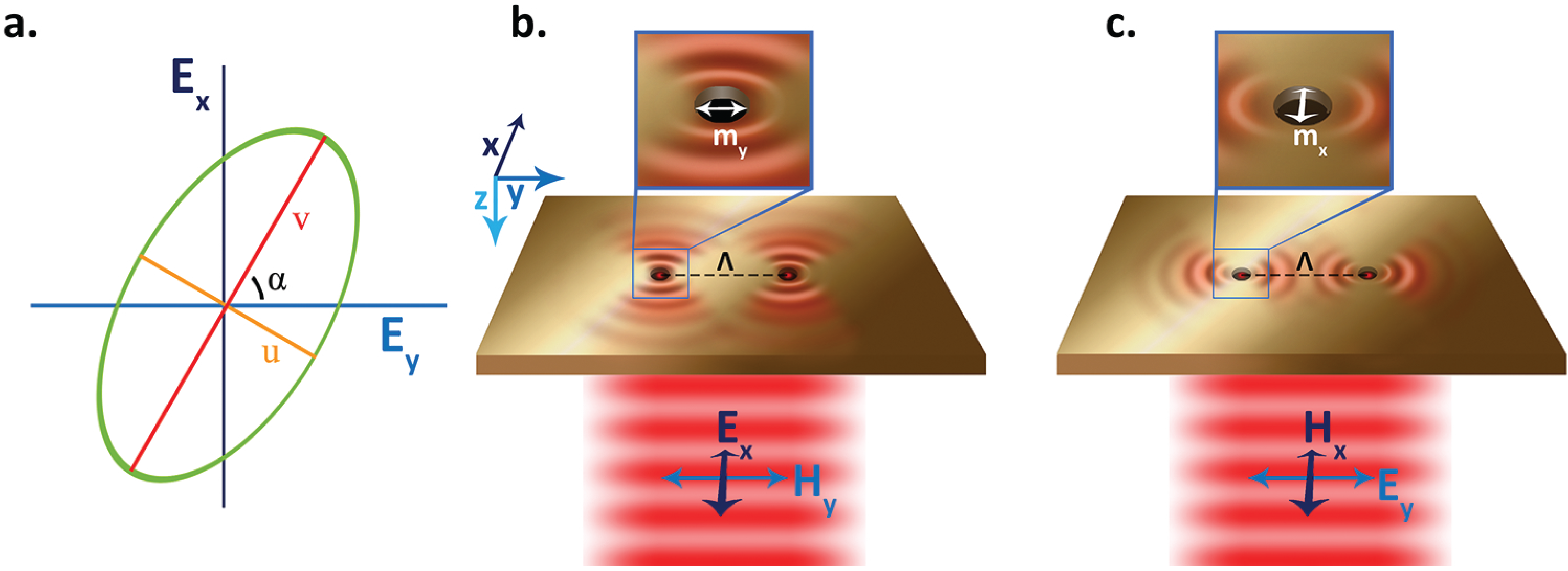
We begin by considering the case shown in Figure 1c, with two holes separated by $\Lambda =3.2$ μm and the incident polarization chosen such that ${\mathbf{H}}^{\mathrm{inc}}=H_x\widehat{x}$, and the holes can interact with each other. The in-plane light field distribution of the SPPs, 20 nm above the gold surface, is shown in Figure 2a, where, in addition to the electric field amplitude, we also show the ellipticity and orientation distributions.

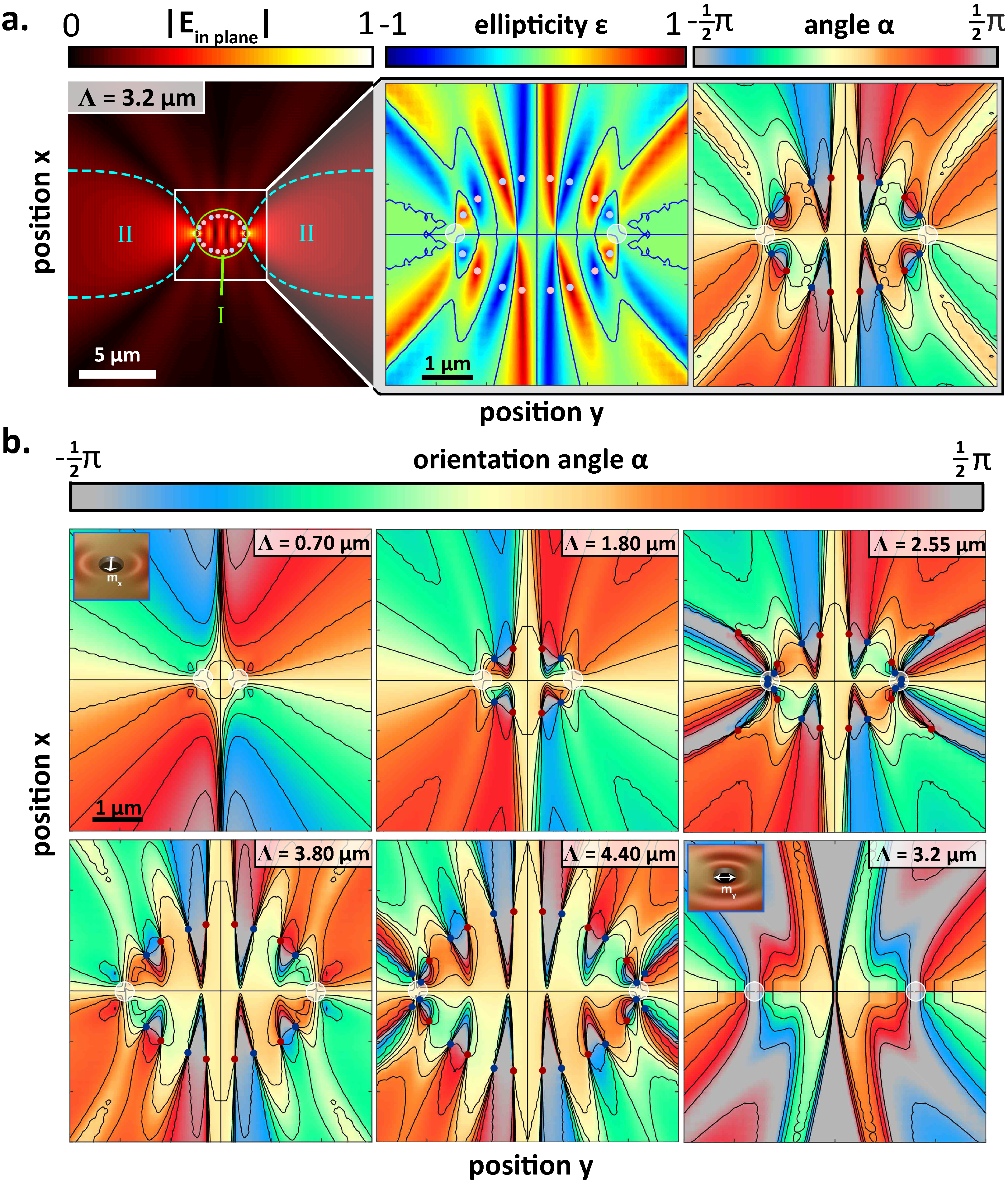
Figure 2. Light field maps for different plasmonic systems. (a) The in-plane electric field amplitude map, along with zoomed in maps of the ellipticity and orientation of the polarization ellipse, for two holes separated by 3.2 μm, with initial excitation $H_x^{\mathrm{inc}}$. In the field amplitude map, we show two curves, $\left(I\right)$ an ellipse and $\left(II\right)$ two parabolas, along which we find polarization singularities. In this figure, we see C-points along I only, and we color code them according to their topological charge, with blue being $+1/2$ and red $-1/2$. We also present ε and α maps in a smaller region of the central area around the holes. For ε, we mark the linear (L)-lines with solid curves, while for α, we likewise show the isogyres. (b) α maps, with circular (C)-points marked in solid symbols as in (a), for Λ ranging from 0.70 μm, where we see no C-points, to 4.40 μm, where we see 28 C-points (24 on I and four on $II$) in our field of view. The last frame shows the case of $\Lambda =3.2$ μm for $H_y^{\mathrm{inc}}$ excitation.

Figure 2. Light field maps for different plasmonic systems. (a) The in-plane electric field amplitude map, along with zoomed in maps of the ellipticity and orientation of the polarization ellipse, for two holes separated by 3.2 μm, with initial excitation $H_x^{\mathrm{inc}}$. In the field amplitude map, we show two curves, $\left(I\right)$ an ellipse and $\left(II\right)$ two parabolas, along which we find polarization singularities. In this figure, we see C-points along I only, and we color code them according to their topological charge, with blue being $+1/2$ and red $-1/2$. We also present ε and α maps in a smaller region of the central area around the holes. For ε, we mark the linear (L)-lines with solid curves, while for α, we likewise show the isogyres. (b) α maps, with circular (C)-points marked in solid symbols as in (a), for Λ ranging from 0.70 μm, where we see no C-points, to 4.40 μm, where we see 28 C-points (24 on I and four on $II$) in our field of view. The last frame shows the case of $\Lambda =3.2$ μm for $H_y^{\mathrm{inc}}$ excitation.

We observe in the field amplitude map that the scattering of SPPs is directional, with most of the light flowing in the $\pm \widehat{y}$ direction, as expected for holes primarily characterized by $m_x$ dipoles. Furthermore, in this amplitude map, we observe side lobes, whose angular position is determined by the interference of the SPPs radiated by the two holes. We note that, as shown in Equation 4, the plasmonic field simply decays exponentially with z, and hence, only the amplitude, but not ε or α, of the field distributions shown in these maps depends on height.

We hunt for C-points, in the plasmonic field radiated by the holes, by looking at the α map (Figure 2a, last panel). In this map, we follow isogyres, lines of constant α, shown with black curves, to their intersections, where α is necessarily undefined, and a C-point is found. For the scattering event shown in Figure 2a, we find 16 C-points that are roughly arranged in an ellipse, with the holes at the tip of the long axis. It is interesting that even such a simple system, with only two holes, can contain such a large number of singularities, and it is particularly useful that some C-points can be almost 2 μm away from the holes. Such relatively large separations are desirable, since, near the hole, other fields, such as cylindrical waves [26], can be present, affecting the field distributions.

When we examine the electric field distributions at, and near, the C-points, we find that, as expected, the C-points occur at locations where $\epsilon =\pm 1$ (Figure 2a, middle panel). Moreover, we find the singularities in pairs, where each pair contains one singularity with a topological index (Equation (3)) of $+1/2$ and one of $-1/2$, which we mark with blue and red symbols, respectively. Hence, the total topological index of the light field is zero.

Having established that, with just two subwavelength holes, we can create electric field distributions that contain multiple C-points, we set out to test the tunability of our system. We begin by varying the separations of the holes, Λ, from 0.6 to 5.0 μm, and calculating the resulting electric field distributions. In Figure 2b, we show a selection of the resultant α maps, in order of increasing Λ. From these images, it is immediately clear that simply changing Λ can greatly affect the resultant light fields, and in particular, we note that the complexity of the α maps increases with larger hole separations.

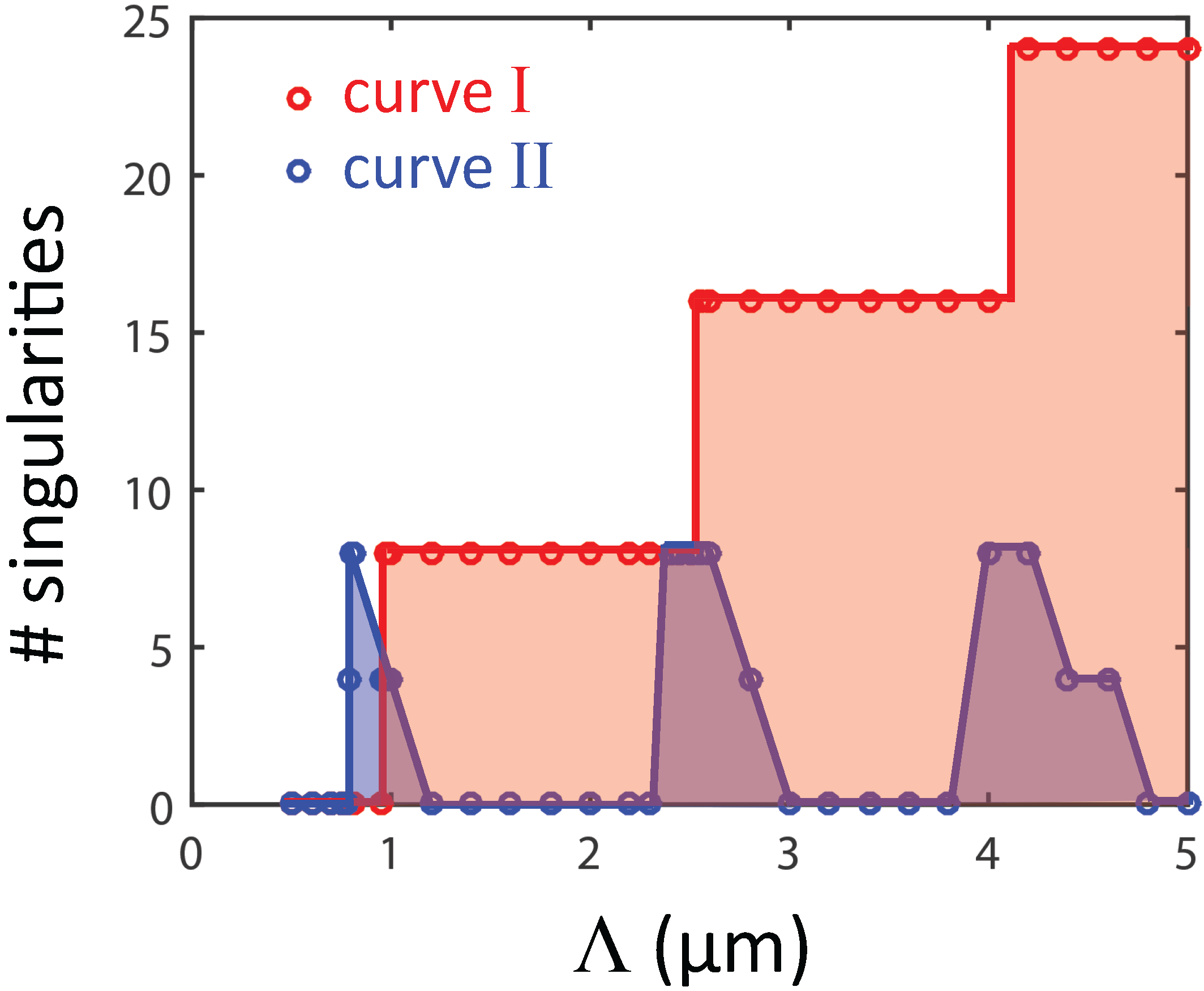
Moreover, we observe a dramatic change in the number of C-points that can be found in each map (Figure 2b). For example, for $\Lambda =0.6$ μm, we do not find any C-points, while for $\Lambda =1.8$ μm, we find eight C-points, and for $\Lambda =3.6$ μm, we find 16 C-points, and so on. This trend is summarized in Figure 3, where it is clear that we find plateaus of Λ where the number of C-points present in the electric field distribution is a constant multiple of eight.

Moreover, in all of these cases, the C-points are found on the ellipse described above, which we sketch out in Figure 2a and mark by curve I. The discrete step size (eight singularities) with which C-points appear can be understood as follows: our plasmonic system has two axes of symmetry ($x=0$ and $y=0$), which lead to a four-fold symmetry of the scattered SPP fields (as is evident from the consideration of a single hole, in Equation (4)). Hence, we expect that if the singularities are created away from the symmetry axes, as is the case here, they will appear at four locations simultaneously. Moreover, at each position of creation, two singularities with an opposite index must be created; otherwise, either the symmetry of our system or the conservation of the index will be violated. Hence, during a creation event, the symmetry of our system and the conservation of the index dictate that a total of eight new C-points appear. Interestingly, the width of each plateau is $\sim {\lambda }_{sp}$, perhaps because, for multiple holes, this would be the threshold for diffraction orders to appear.

Figure 3. Number of C-points in our field of view, for the plasmonic system introduced in Figure 2, as a function of Λ, showing clear plateaus of multiples of eight. Both the C-points found along curve I are shown (in red), as are those along curve $II$ (in blue).

Figure 3. Number of C-points in our field of view, for the plasmonic system introduced in Figure 2, as a function of Λ, showing clear plateaus of multiples of eight. Both the C-points found along curve I are shown (in red), as are those along curve $II$ (in blue).

In the α maps presented in Figure 2b and in Figure 3, we observe that something interesting occurs near transitions when the number of C-points increases. The transition is, in fact, not straight from n to $n+8$ C-points. Rather, at first, when a transition occurs, several extra C-points appear, which then disappear when the new, $n+8$ plateau is reached. For example, when $\Lambda =2.55$ μm (Figure 2b, last image in the top row), we observe 20 C-points and not the 16 of the plateau (e.g., $\Lambda =3.8$ μm; Figure 2b, first image bottom row). Interestingly, these ‘extra’ C-points are always found outside of the main C-point ellipse, on curve $II$, as marked in Figure 2a, and first appear far away, at large y values. These extra C-points then move closer and closer to the holes, until after the creation event, when, continuing on curve $II$, they again move out of our field of view. The creation of C-points will be discussed in more detail, in Section 3.3 below.

Finally, we recall that it is also possible to change the excitation beam, such that ${\mathbf{H}}^{\mathrm{inc}}=H_y\widehat{y}$, corresponding to the last panel of Figure 2b. In this case, the incident beam will predominantly excite the $m_y$ dipole in the holes, and they will not interact. As expected for this incident polarization, SPPs are radiated by the holes predominantly in the $\pm \widehat{x}$ directions. More importantly, in the α maps, an example of which is shown in the last image in the bottom row of Figure 2b for $\Lambda =3.2$ μm, we find no C-points. This is true for the entire range of Λ’s that we investigate (from $\Lambda =0.6$ to $5.0$ μm). That is, two plasmonic holes that, initially, scatter SPPs perpendicularly to the line on which they lie are not sufficient to create electric field distributions that support C-points. Moreover, using a two-hole plasmonic system, it is therefore possible to create and annihilate C-points simply by rotating the polarization of the excitation beam.

3.2. Three Holes

It is, of course, also possible to increase the number of holes in the gold film. We can preserve the symmetry of our system, even as we add holes, by placing the additional holes on the $x=0$ line, along with the original two holes. The additional holes act as extra sources of SPPs, both initially or from secondary scattering events in the case of hole-hole interactions, resulting in more complex field distributions. We show examples of such fields (including the amplitude, ε and α), for the case of three holes separated by $\Lambda =3.2$ μm, for initial excitation using $H_x^{\mathrm{inc}}$ in Figure 4a and $H_y^{\mathrm{inc}}$ in Figure 4b.

In these, we observe that the directionality of the scattering is still determined by the excitation, with SPPs being radiated primarily in the $\pm \widehat{y}$ direction for $H_x^{\mathrm{inc}}$ excitation, and vice versa, but that many more side lobes arise in comparison to the field profiles created by the two plasmonic holes (Figure 2a).

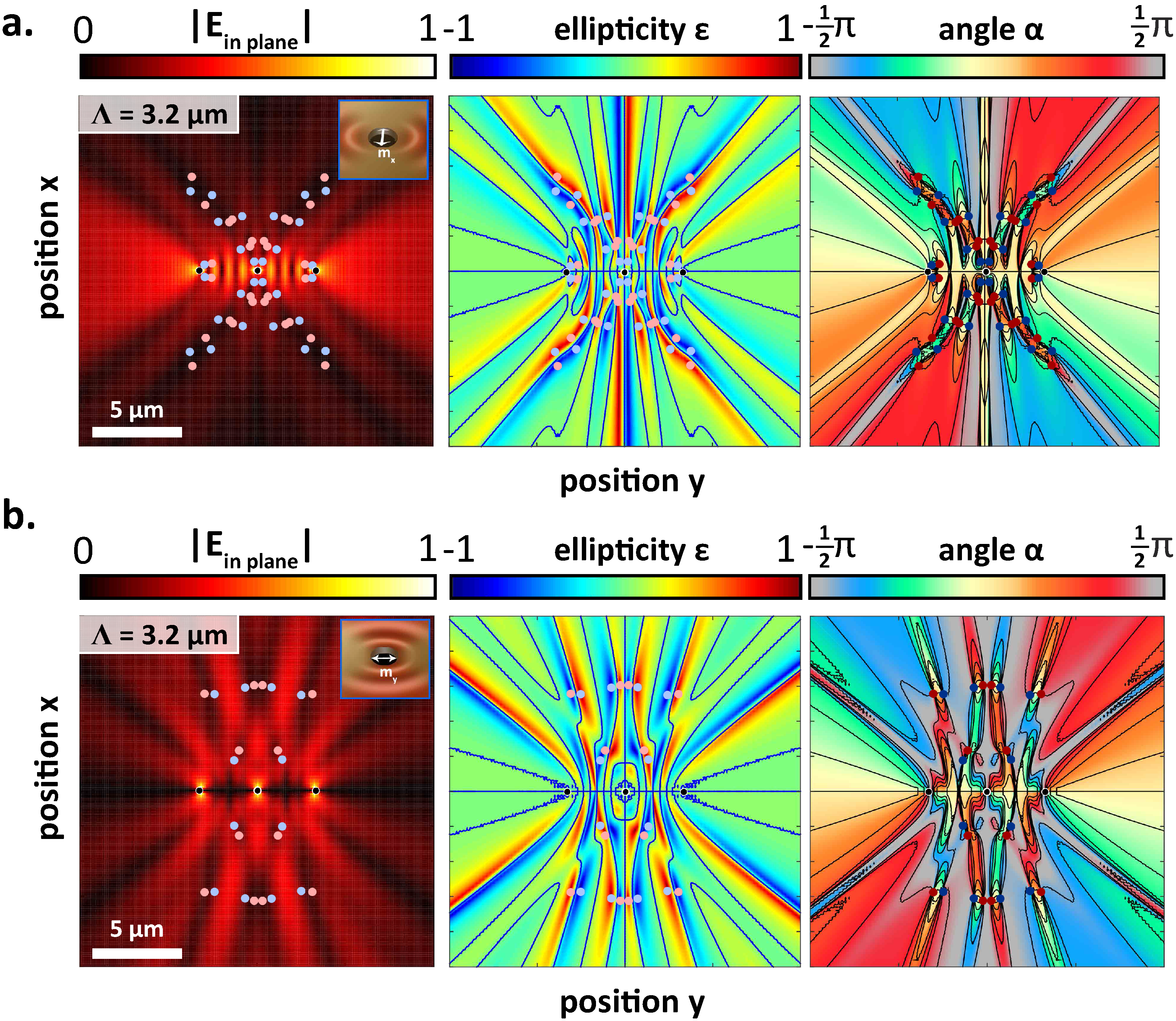
Figure 4. Light fields around three holes. Field amplitude, ε and α maps for three holes with 3.2-μm separations when the incident response of the holes is dominated by (a) $m_x$ and $m_y$ dipoles. Both sets of maps clearly contain many C-points.

Figure 4. Light fields around three holes. Field amplitude, ε and α maps for three holes with 3.2-μm separations when the incident response of the holes is dominated by (a) $m_x$ and $m_y$ dipoles. Both sets of maps clearly contain many C-points.

Given the increased complexity of the electric field distribution for the three-hole systems, we could expect to find additional C-points therein, relative to the case when only two holes were present. In fact, searching the field maps for both the two- and three-hole systems reveals that this is the case: for example, for the two-hole system with $\Lambda =3.2$ μm (Figure 2a), we observed 16 C-points, while for the same Λ, when ${\mathbf{H}}^{\mathrm{inc}}=H_x\widehat{x}$ (Figure 4a), we now observe 56 C-points. Moreover, we see that when three holes are present, we find C-points at greater distances from the holes, particularly in the $\widehat{x}$ direction. In essence, the SPPs scattered from the two outer holes can interfere with the field from the middle hole, at relatively large distances directly above (or below, $\left|x\right|>0$) it, to create circular polarized light.

Interestingly and in contrast to the case when only two holes were present, with three holes, we observe C-points even for ${\mathbf{H}}^{\mathrm{inc}}=H_y\widehat{y}$ excitation, where the holes do not interact. In Figure 4b, for example, we find 24 C-points, which is comparable to the number of C-points found for only two holes under ${\mathbf{H}}^{\mathrm{inc}}=H_x\widehat{x}$ excitation at this separation. It is clear that, regardless of the excitation field orientation, light fields containing polarization singularities can be created with relatively few such sources.

3.3. Creation and Annihilation of C-Points

The simple way in which our plasmonic system can be used to create light fields that contain polarization singularities, and, more specifically, how nanoscale geometry controls these features, allows it to be used as a platform to study properties of these C-points. As a demonstration, we focus on the creation of C-points and study the evolution of the light fields as new singularities appear due to changes in geometry. Specifically, we consider the situation first shown in Figure 2b and Figure 3, where, near $\Lambda =2.5$ μm, new C-points appear.

By $\Lambda =2.7$ μm, whose field amplitude and polarization maps we show in Figure 5a, the transition from eight to 16 C-points on curve I has been completed. At $\Lambda =2.7$ μm, we observe that the 16 C-points are arranged nicely in an elliptical curve and are found in pairs of opposite charge, where, in each pair, one C-point is found where $\epsilon =1$ and the other where $\epsilon =-1$. As we learned, from Figure 2, the new C-points appear near the holes, and so, we now focus on a small area near the leftmost hole, as marked by the red rectangle in the α map (Frame 3) of Figure 5a, and we study the evolution of the light fields, as the C-point pair shown in this volume appears (Figure 5b).

At hole separations before the appearance of the new C-point pair, for example at $\Lambda =2.52$ μm, as shown in the first pane of Figure 5b, we see no points where α is undefined, in our region of interest. At $\Lambda =2.53$ μm (second frame, Figure 5b), however, something interesting occurs. This small change of separation, from 2.52 to 2.53 μm, is not enough to cause C-points to appear (at least, not within the resolution of our calculations), but it is enough to cause a point to appear in the α map, where the orientation is somewhat jumbled. We mark this point with a green circle, and as we see from the subsequent frames, it is from this point that the light fields that contain the C-points evolve.

In fact, a further small increase in separation, to $\Lambda =2.55$ μm (third frame, Figure 5b), is sufficient to make C-points clearly visible in the polarization maps. We mark these with blue and red circles and note that they carry a topological index of $+1/2$ and $-1/2$, respectively, ensuring that the total topological index of the light field is conserved in this creation process. Interestingly, both C-points are formed in regions where $\epsilon =-1$; that is, although the C-points carry the opposite index, the light fields in their vicinities have only one handedness. This situation remains even for $\Lambda =2.60$ μm (fourth frame, Figure 5b), although as Λ increases, so too does the separation between the new C-points.

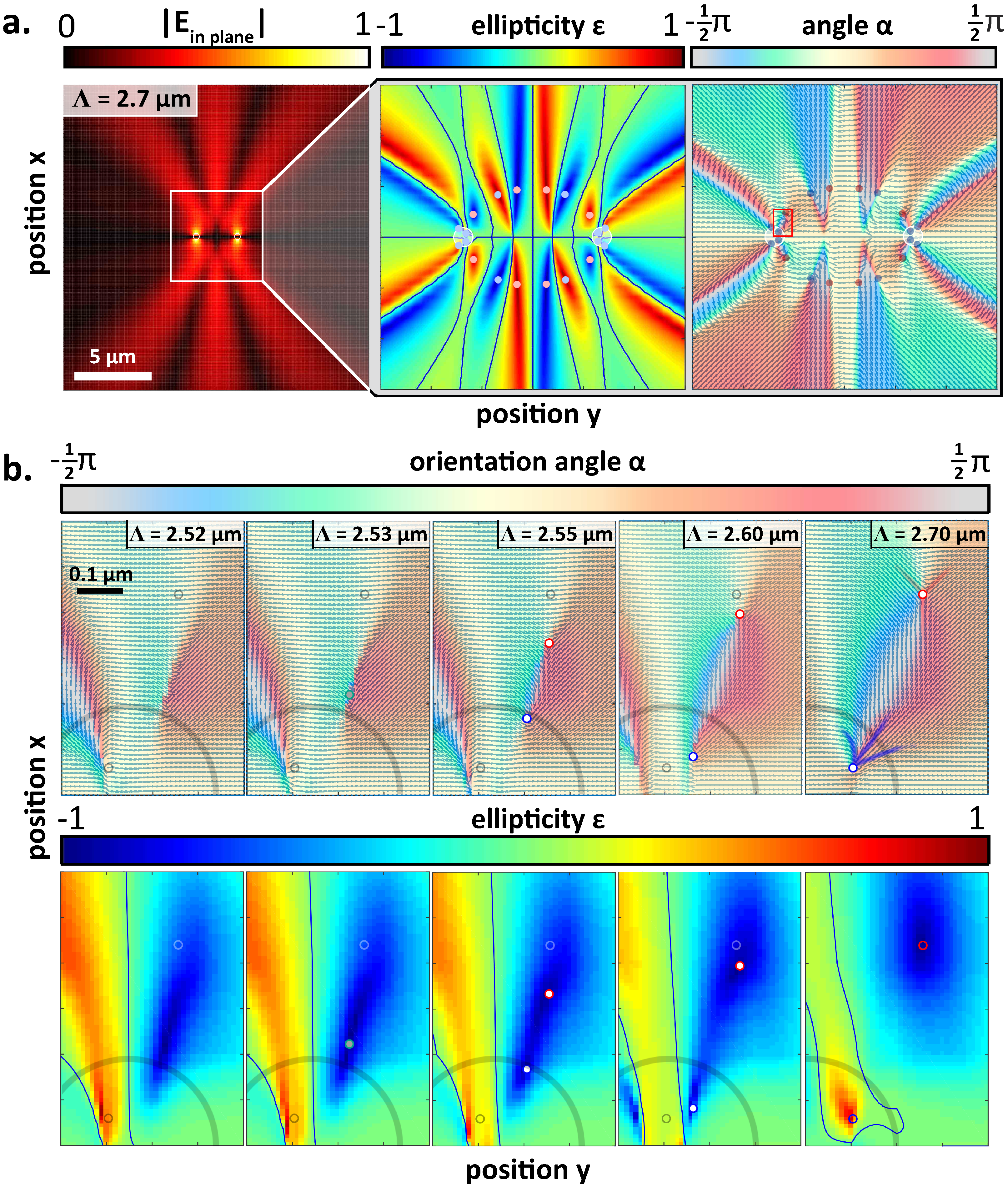
Figure 5. Evolution of the electric field leading to the creation of C-point pairs. (a) The in-plane electric field amplitude map, along with zoomed in maps of the ellipticity and orientation of the polarization ellipse, for two holes separated by 2.7 μm, with initial excitation $H_x^{inc}$. In the ε and α maps, we mark the locations of the C-points, and for α, we also overlay the color map with vectors aligned along the direction of the long axis. Additionally, the region that contains the two C-points whose creation we investigate is marked in the α map. (b) The spatial evolution of ε and α for $\Lambda =2.52$ to $2.70$ μm, in the region marked in (a). In all panes, we show the outlines of the holes, which scans through the field of view with the change to Λ. In all panes, we also show the final positions of the two C-points (for $\Lambda =2.7$ μm). For $\Lambda =2.53$ μm, we mark the location where changes in the α map herald the formation of the C-points, which we subsequently also mark for larger separations. Finally, for $\Lambda =2.70$, we also trace out the lines of constant α leading to the singularity, observing that the top C-point is a star singularity, while the bottom C-point is of the monstar variety.

Figure 5. Evolution of the electric field leading to the creation of C-point pairs. (a) The in-plane electric field amplitude map, along with zoomed in maps of the ellipticity and orientation of the polarization ellipse, for two holes separated by 2.7 μm, with initial excitation $H_x^{inc}$. In the ε and α maps, we mark the locations of the C-points, and for α, we also overlay the color map with vectors aligned along the direction of the long axis. Additionally, the region that contains the two C-points whose creation we investigate is marked in the α map. (b) The spatial evolution of ε and α for $\Lambda =2.52$ to $2.70$ μm, in the region marked in (a). In all panes, we show the outlines of the holes, which scans through the field of view with the change to Λ. In all panes, we also show the final positions of the two C-points (for $\Lambda =2.7$ μm). For $\Lambda =2.53$ μm, we mark the location where changes in the α map herald the formation of the C-points, which we subsequently also mark for larger separations. Finally, for $\Lambda =2.70$, we also trace out the lines of constant α leading to the singularity, observing that the top C-point is a star singularity, while the bottom C-point is of the monstar variety.

By $\Lambda =2.70$ μm (last frame, Figure 5b), the C-points are well separated and, interestingly, can now be found in regions of opposite handedness. The flip in handedness of the field in the area of the bottom C-point is interesting, because, for this to occur, it seems as though the C-point must cross an L-line; this view is supported by Figure 5b, where up to separations of 2.60 μm, there is no L-line between the C-points, while it is clearly there when $\Lambda =2.70$ μm. Such a crossing of a C-point and an L-line is, in fact, not possible, since on the L-line, the polarization of the light is linear and, hence, has a well-defined orientation. Consequently, a C-point cannot be found on an L-line.

A closer look at the evolution of the C-points after their creation, in high-resolution simulations, allows us to determine how the handedness of the bottom C-point in Figure 5b flips. Initially, in the region shown in the figure, we observe two C-points on fields characterized by $\epsilon =-1$. Outside our field of view, below the y-axis, the situation is reversed, and two C-point on fields where $\epsilon =1$ were created. The handedness of the field underlying each singularity is, in fact, unchanged as the singularity moves due to a tuning of Λ. Rather, as Λ is increased, the two C-points closest to the y-axis—the one above, in our field of view, and the one below—switch partner singularities. Once this switch occurs, at $\Lambda =2.64$ μm, each singularity pair contains fields of both handedness, which are separated by an L-line. We emphasize that, during this rearrangement, no C-points are created or annihilated (further details and images of the way that the C-points switch their partner singularity can be found in the Supplementary Information).

Finally, for the $\Lambda =2.70$ μm frame in Figure 5b, we trace the lines of constant α in the vicinity of the C-points to identify the type of singularity. We see that the top singularity is a star-type C-point, identified by the three-fold symmetric straight lines that radiate away from the singularity, while the bottom point is monstar C-point, where, again, three straight lines radiate away from the singularity, though without the three-fold symmetry of the star. Interestingly, when further increasing Λ to, for example, $3.0$ μm, we observe that the bottom C-point has transformed from a monstar to a lemon-type C-point (see the Supplementary Information). The evolution of the singularities, from the creation of a star-monstar pair to the subsequent transformation of the monstar to a lemon, confirms earlier predictions of this event [19].

4. Conclusions

In this article, we present a new plasmonic platform that can be used to study polarization singularities in nanoscale light fields: an arrangement of multiple subwavelength holes on optically thick metal films. We show that depending on the polarization of the excitation beam, two or three holes are sufficient to create light fields with C-points. Moreover, we demonstrate that these light fields are intimately linked to the exact geometry of the system and that small changes in the hole separations are enough to create or annihilate many C-points. In fact, in the case of a system of two plasmonic holes, we observe large plateaus of integer multiples of eight C-points in the light fields, with sharp transitions that can contain additional C-points, as a function of the inter-hole separations. Finally, we show that using this system, we are able to study the evolution of the light field during one of these creation transitions. We focus on the transition from 16 to 24 C-points, for two holes, which occurs for hole separations of about 2.5 μm, where we can pinpoint the location where the creation occurs, as well as the type of C-points and the underlying helicities of the local light fields.

In conclusion, our results open up a new system where fundamental properties of light fields can be studied at length scales compatible with near-field microscopy techniques [17,20,27,28]. Moreover, many recent nanophotonic applications, from biosensing using chiral fields [29] to on-chip control of dipole emission [30,31] for quantum optics, rely on highly structured local light fields near nanoscopic structures. In these applications, the fine structure of near fields is used to control the interaction of the nanophotonic structure with a nearby objects, be it a molecule or emitter. Our system, therefore, offers another approach to creating, and studying, such light fields, and may therefore be of interest as a route towards new technologies.