Circuit Model of Plasmon-Enhanced Fluorescence

Abstract

Hybridized decaying oscillations in a nanosystem of two coupled elements—a quantum emitter and a plasmonic nanoantenna—are considered as a classical effect. The circuit model of the nanosystem extends beyond the assumption of inductive or elastic coupling and implies the near-field dipole-dipole interaction. Its results fit those of the previously developed classical model of Rabi splitting, however going much farther. Using this model, we show that the hybridized oscillations depending on the relationships between design parameters of the nanosystem correspond to several characteristic regimes of spontaneous emission. These regimes were previously revealed in the literature and explained involving semiclassical theory. Our original classical model is much simpler: it results in a closed-form solution for the emission spectra. It allows fast prediction of the regime for different distances and locations of the emitter with respect to the nanoantenna (of a given geometry) if the dipole moment of the emitter optical transition and its field coupling constant are known.

1. Introduction

Plasmon-enhanced fluorescence has a rather long history, and the amount of papers dedicated to this phenomenon is huge (see, e.g., [1]). In the simplest and most practical case, this fluorescence is obtained in a structure comprising two optically small elements coupled by the dipole-dipole interaction. Element 1 is the fluorescent quantum emitter (QE), and Element 2 is the optically small plasmonic nanoantenna (NA), also called the nanocavity or nanoresonator. Often, the radiated power of plasmon-enhanced fluorescence can be calculated via the so-called Purcell factor $F_P$ [2]. The Purcell factor describes the decay rate of the spontaneous emission in the presence of the NA [3]. Its increase is equivalent to the gain in the radiated power at the emission frequency [4]. The enhancement of the fluorescence by the NA implies $F_P>1$ (direct Purcell effect), and the suppression (inverse Purcell effect) corresponds to $F_P<1$ [3,5,6,7]. When $F_P\ll 1$, i.e., the decrease of the emission makes it not measurable, the inverse Purcell effect is called fluorescence quenching (see, e.g., [8,9,10,11,12]). The cases when the spectral line of the fluorescence nearly keeps its shape and only the level is modified is usually called the weak coupling regime [4]. Is it coupling between Elements 1 and 2?

Usually (see, e.g., [3,5,6,7]), weak and strong coupling regimes are distinguished by comparing the so-called emitter-field coupling constant $\chi ={\left[\right|\mathbf{d}|}^2{\omega }_0/\left(2\hslash {\epsilon }_0{\epsilon }_{r}V\right){]}^{1/2}$ with the decay rate of the NA ${\gamma }_2$ and the non-radiative (due to dissipation) decay rate of the excited state of the QE ${\gamma }_{\mathrm{1dis}}$ [4]. Here, ${\omega }_0$ and $\mathbf{d}=e\langle 2\left|\mathbf{r}\right|1\rangle$ are the frequency of the excited-to-ground state transition ($2\to 1$) and its dipole moment (matrix element), respectively, e is the electron charge, V is the effective volume of the resonator mode, ${\epsilon }_0$ is the vacuum permittivity and ${\epsilon }_r$ is the relative permittivity of the host medium. (We use the SI units; the result in the CGSunits can be obtained by replacing ${\epsilon }_0$ by $1/\left(4\pi \right)$.)

The case of the weak emitter-field coupling (WEFC) corresponds to $\chi <{\gamma }_{\mathrm{1dis}}$. In practical cases, the dissipative losses in both QE and NA are much smaller than the radiative ones. Then, the WEFC condition can be written as $\chi \ll {\gamma }_1$, where ${\gamma }_1$ is total decay rate of Object 1. In this condition, the frequency of the spontaneous emission remains equal to ${\omega }_0$, and the interaction may only lead to a certain modification of the decay rate. Respectively, the dipole moment of the optical transition d of the QE and its classical dipole moment ${\mathbf{d}}_1$ remain unperturbed. At the emission frequency ${\mathbf{d}}_1\left({\omega }_0\right)=2\mathbf{d}$, and the shape of the emission line remains Lorentzian [4]. However, does the weakness of the emitter-field coupling obviously mean the weak mutual coupling (WMC) between the QE and the NA and vice versa? This question needs to be analyzed.

In the case of the strong emitter-field coupling (SEFC), $\chi >{\gamma }_2$. It is known that the mutual coupling is described by another constant ${\omega }_R$ called the Rabi constant [4,13,14]. The strong mutual coupling (SMC) of Objects 1 and 2 holds when ${\omega }_R\gg {\gamma }_{1,2}$. Does SEFC obviously imply the SMC regime?

In the case of the strong mutual coupling (SMC), the spectrum of the plasmon-enhanced fluorescence is noticeably hybridized [13] and corresponds to so-called Rabi oscillations. In quantum optics Rabi oscillations are usually referred to as the amplitude modulation of the emission, which arises when the emitter is excited by an incident wave whose frequency lies within the emission spectrum [4,14]. In this resonant case, the emission is periodic and represents a beating oscillation. The simplest case is that of the coherent pumping when the incident wave has the frequency exactly equal to ${\omega }_0$. The Rabi modulation corresponds to frequencies ${\omega }_{\pm }={\omega }_0\pm {\omega }_R$, where ${\omega }_R=\mathbf{d}·{\mathbf{E}}^V/\hslash$ is called either the Rabi interaction constant or Rabi frequency [4]. It represents one half of the beat frequency of the modulated emission. Here, ${\mathbf{E}}^V$ is the incident wave electric field amplitude (also called the vacuum field) at the QE origin. Physically, the beating of the spontaneous emission corresponds to the periodic energy exchange between the QE and the wave. During one half of the modulation period $\pi /2{\omega }_R$, the QE borrows the power from the wave and in the next half-period returns it.

A similar modulation process may hold in the nanosystem of the QE coupled to the NA, whereas the role of the incident wave is played by the secondary field of the NA [13]. This phenomenon was called self-induced Rabi oscillations in the pioneering work [13]. It was later studied in many works using the semiclassical model, which allows the quantitative agreement with the experiment (see, e.g., [7,11,12,16,17]).

Definitely, the Rabi oscillations in the nanosystem QE plus NA can be interpreted as a purely classical effect of splitting the eigenmode of two coupled oscillators. This effect is well known, and it is not surprising that there were several attempts to use the classical model instead of the semiclassical approach. The classical model is deterministic and rather simple, whereas the semiclassical model results in the system of Langevin–Schrödinger equations of motion and requires difficult numerical simulations. The classical model correctly describes the conditions of the Rabi splitting. In [13,14], the authors successfully compared the bounds for the observed Rabi splitting to the predictions of the classical model [15]. Notice that this classical model was initially developed not for the nanosystem of the QE coupled to the NA. It was suggested in [15] for the mutual interaction of so-called Rydberg’s atoms and only later, in [18], extended to the cavity-enhanced fluorescence. Notice that the applicability of this model to Rydberg’s atoms is a priori much wider than to plasmon-enhanced fluorescence, because these atoms are basically classical scatterers.

In [18], the authors considered a chain of N different springs loaded by N masses all coupled by equivalent springs to a common mass. Alternatively, it can be referred to as a chain of series electric circuits coupled by mutual inductances to a common circuit. This model was applied to describe the nanosystem of N QEs interacting with the same single-mode resonator (such as a small semiconductor cavity). It was shown that in the case of high dissipation in QEs, this classical model correctly predicts the absorption spectrum of the array of fluorescent molecules located in the cavity. Later, this approach was developed for the case $N=1$ and applied to our nanosystem in [16,19,20,22]. It was shown that the classical model in this case also properly predicts the conditions of the Rabi splitting and the absorption spectra. However, the applicability of the model for spectra of plasmon-enhanced fluorescence was not analyzed. How does one calculate these spectra in the case of SMC?

It is clear that between the weak and strong coupling regimes, there should be one or more regimes that correspond to the intermediate coupling of the QE to the field. What happens with the emission rate and spectrum in this intermediate case?

The semiclassical model answers all of these questions only after challenging simulations. The known classical model [15,16,18,19,20,22] replacing the actual dipole-dipole interaction by the elastic coupling, in our opinion, cannot properly predict the fluorescence spectra. We suggest a more elaborated model, which also borrows one basic formula from quantum mechanics: a static polarizability of a two-level system. The use of this formula allows us to fully fit the model to quantum optics. Similar to the known elastic model, our model also results in closed-form solutions; however, unlike it, our solutions, in our opinion, should cover all known regimes beyond the case of a strong tunneling effect. At least the three most important regimes of plasmon-enhanced fluorescence—the Purcell effect, Rabi splitting and fluorescence quenching—are described by our model.

2. Theory

2.1. Elastic/Inductive Coupling

Let us reproduce the result of the known classical model of Rabi oscillations (see, e.g., [4,15,16,18,19]), which is considered in these and further works as a classical analogue of the quantum system under study. Oscillators (e.g., two $LRC$-circuits or two springs with masses coupled by the third spring) are described by a well-known system of differential equations:

$$\left\{\begin{array}{c}\frac{{\partial }^2{x}_1}{\partial t^2}+{\gamma }_1\frac{\partial x_1}{\partial t}+{\omega }_{01}^2{x}_1-q_1^2{x}_2=0,\\ \frac{{\partial }^2{x}_2}{\partial t^2}+{\gamma }_2\frac{\partial x_2}{\partial t}+{\omega }_{02}^2{x}_2-q_2^2{x}_1=0\end{array}\right.$$

(1)

For simplicity of writing, it is reasonable to restrict the analysis by the case of the exact resonance: the eigenfrequencies of two oscillators are equivalent ${\omega }_{01}={\omega }_{02}={\omega }_0$. To avoid ambiguity, let us agree that two coupled oscillators are circuits coupled by their mutual inductance M. Then, ${\omega }_0=1/\sqrt{L_1{C}_1}=1/\sqrt{L_2{C}_2}$, ${\gamma }_{1,2}={\omega }_0{C}_{1,2}{R}_{1,2}$ are Lorentz’s decay factors of Circuits 1 and 2. Furthermore, in this case, $q_1=q_2=q\equiv {\omega }_{0}M/\sqrt{L_1{L}_2}$ is the factor of mutual interaction having the dimensionality of frequency, as well as the decay factors. The replacement of the time derivative by $j\omega$ (the time dependence $\exp \left(j\omega t\right)$ is selected) and equating the determinant to zero results in the equation for eigenmodes. Two physically-sound solutions in the case ${\gamma }_{1,2},q\ll {\omega }_0$ take form (see, e.g., [16,18,19]):

$${\omega }_{\pm }={\omega }_0-j\frac{{\gamma }_1+{\gamma }_2}{4}\pm \sqrt{q^2-{\left(\frac{{\gamma }_1-{\gamma }_2}{4}\right)}^2}$$

(2)

Equation (2) is, in fact, approximate, though its limits of validity have not been discussed in [16,18,19]. The exact expression for the roots of the dispersion equation is derived and discussed below. Since, namely, the Equation (2) has been analyzed in the literature, in this section, we briefly reproduce this analysis. Below, a more elaborated original analysis is presented, and the reader may judge which of them is more relevant. If $q<|{\gamma }_1-{\gamma }_2|/2$ (this case in the literature is referred to as weak mutual coupling), ${\omega }_{\pm }={\omega }_0-j({\gamma }_1+{\gamma }_2)/4\pm j\xi$, where $\xi =\sqrt{{\left[({\gamma }_1-{\gamma }_2)/4\right]}^2-q^2}$. Since $\xi <({\gamma }_1+{\gamma }_2)/4$, both roots are physical. In this case, the hybridization results in the distortion of the Lorentzian line shape. This distortion is noticeable for q approaching $|{\gamma }_1-{\gamma }_2|/4$. Another result is the modification of the effective decay rate, i.e., Purcell’s effect. The regime of weak mutual coupling when the Purcell effect is, however, noticeable was called overdamped in [18].

If $q>|{\gamma }_1-{\gamma }_2|/2$ (this case is usually referred to as strong mutual coupling; however, below, we explain that the applicability of this terminology needs to be revised), there are two complex eigenfrequencies with distinct real parts $\mathrm{Re}\left({\omega }_{\pm }\right)$. The case $q\gg |{\gamma }_1-{\gamma }_2|/2$ is referred to in the literature as ultra-strong coupling (we explain below how to avoid this ambiguous terminology), when one can neglect the small imaginary part of ${\omega }_{\pm }$ and write an approximate formula of Rabi splitting:

$${\omega }_{\pm }\approx {\omega }_0\pm q$$

(3)

The factor q is identified with the Rabi frequency ${\omega }_R$ in [11,14,15,16,18,19,20,22]. However, in none of them is q calculated through the parameters of the nanosystem and compared with the known result of quantum optics for ${\omega }_R$. It is difficult to compare the elastic model with the quantum one because it is not clear how to calculate the effective mutual elasticity or mutual inductance M of two quantum oscillators. There is even no evidence that this coupling is elastic/inductive. The only argument in favor of the elastic model is the symmetry of coupling corresponding to Rabi oscillations [15,18,20]. Notice that such a mechanical analogue of two coupled series $LRC$-circuits as a system of two non-identical pendulums with masses $m_{1,2}$ and lengths $D_{1,2}$ coupled by a spring of elasticity M is described by the set of Equation (1), where two coupling parameters $q_1\ne q_2$ are not equivalent in the case of the exact resonance ($(g{m}_1+M{D}_1)m_2{D}_2=(g{m}_2+M{D}_2)m_1{D}_1$), namely $q_{1,2}=M{D}_{1,2}/m_{1,2}{D}_{2,1}$. If these parameters are equal (symmetric coupling), the exact resonance is not achievable, except the trivial case of two identical pendulums. The asymmetry of coupling is an argument against this model, considered earlier only as a classical illustration of the quantum effect.

Equation (2) implies that the spectrum of fluorescence for both overdamped and hybrid regimes should be different from Lorentzian. The same observation refers also to the absorption spectrum (when the system is excited by an incident wave). For the absorption spectra, the fully classical model turned out to be adequate. At least it was so for the special cases studied in [16,18,22]. For the spectra of spontaneous emission, this model probably fails, since we have found in the literature not one successful attempt to apply the elastic model for the evaluation of these spectra.

The first known attempt to develop the circuit model of emission beyond the approximation of two elastically-coupled elastic oscillators was done in [21]. However, this work, though widely cited, is wrong. The equivalent scheme of the dipole-dipole interaction suggested in [21] does not stand an express analysis. First, in [21], the circuits describing the spontaneous emission (fluorescence) and the response to the external field are drastically different, whereas the correct scheme of the nanosystem treating it as a pair of dipole scatterers with perhaps internal sources is obviously unique. Second, the impedance of free space is mistakenly included as a series load into the emitter circuit. This connection obviously causes non-physical fluorescence spectra.

In fact, the radiation to free space in the circuit model is described not by the free-space impedance, but by the radiation resistance. Moreover, the radiation resistance enters similarly Lorentz’s decay factor γ of both Elements 1 and 2, whereas in [21], free-space impedance is included only in the emitter circuit. A physically-sound circuit model that corrects and replaces the wrong model [21] was suggested in our precedent work [23]. This model shows that the dipole-dipole coupling of two circuits comprises all components: inductive, capacitive and resistive. The resistive component allows the resonant enhancement of the effective radiation resistance of the QE and results in the Purcell effect.

2.2. Circuit Model of Coupling in Plasmon-Enhanced Fluorescence

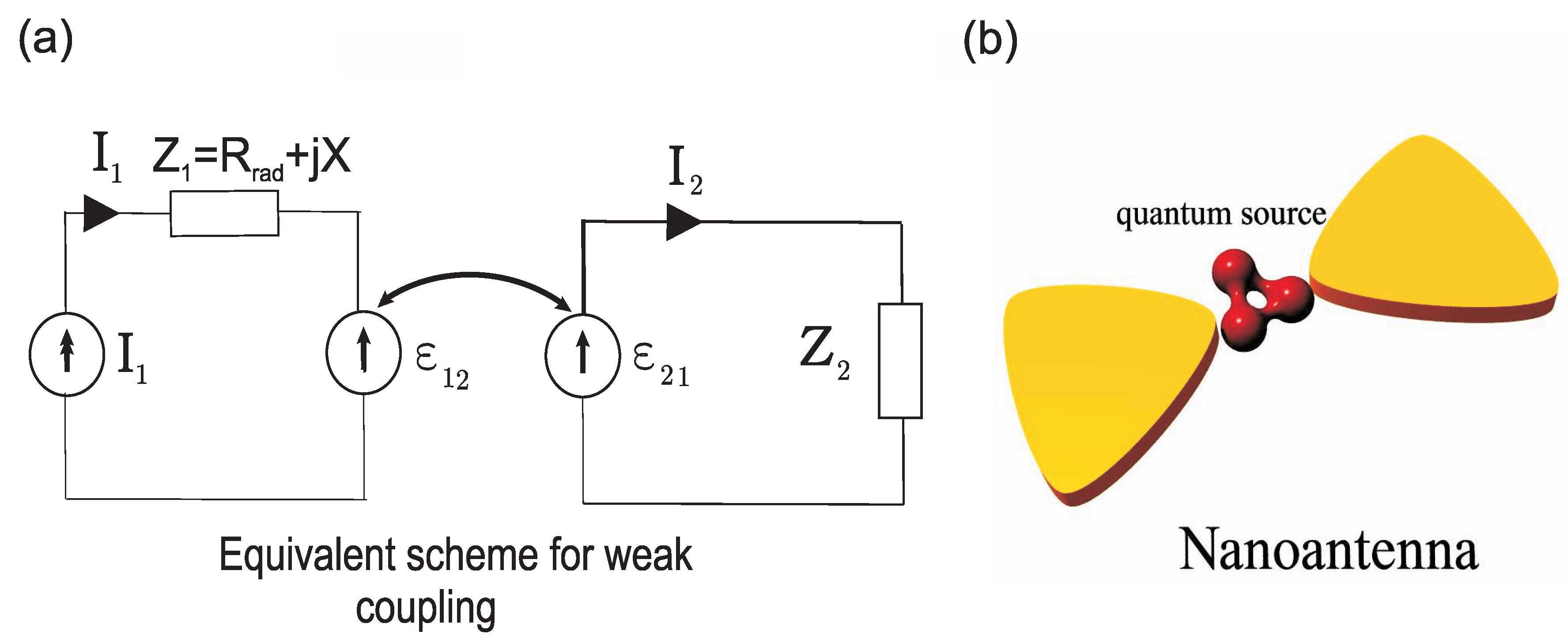
The equivalent scheme of the QE (Object 1) coupled to a plasmonic NA (Object 2) suggested in [23] is shown in Figure 1a. This scheme is unique for both emission and scattering. The applicability of this scheme is restricted by the case of weak mutual coupling (WMC) of the QE and the NA. This restriction is related to the approximation of the ideal current generator. The WMC approximation discussed above implies the unperturbed dipole moment of the NA ${\mathbf{d}}_1$. Really, the dipole moment $d_1$ characterized by the certain effective length $l_1$ of Dipole 1 (it enters the Lorentzian polarizability model of the QE [23]) is linked to the effective current $I_1$ as $d_1=I_1{l}_1/j\omega$. Therefore, the unperturbed $d_1$ implies the approximation of the current generator exciting the QE. This approximation was successfully used in [23] in order to obtain the high Purcell factor of the QE enhanced by a plasmonic NA. Below, we will show that this result corresponds to the case when the condition of WMC is combined with the condition of intermediate emitter-field coupling (IEFC).

Our circuit model was validated in [23] by comparison with the exact solution for an explicit example: a quantum dot located at an optically small, but sufficient (for the weak-coupling regime) distance $G=10$ nm from a golden nanosphere of a diameter of 40 nm. We obtained a very good agreement for the Purcell factor over the whole spectrum. Here, it is worth noticing that the fluorescence line, though it is a quantum effect, has a Lorentzian spectral shape.

Figure 1. (a) Equivalent scheme of a weakly-coupled quantum emitter and nanoantenna. (b) One of the possible realizations of the spacer.

Figure 1. (a) Equivalent scheme of a weakly-coupled quantum emitter and nanoantenna. (b) One of the possible realizations of the spacer.

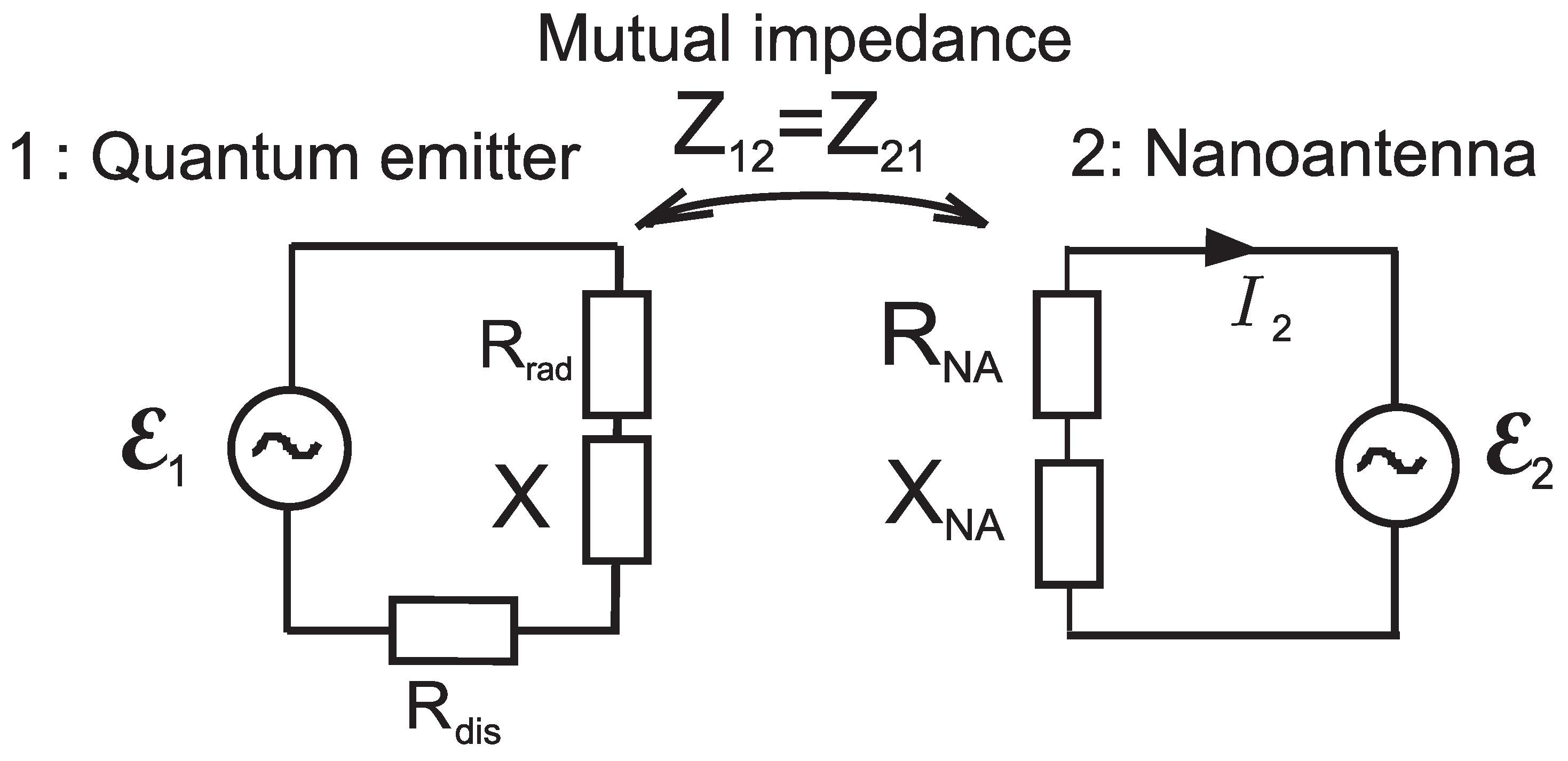
Figure 2. An equivalent scheme of a system of two coupled oscillators whose mutual interaction is described by mutual impedance $Z_{12}=Z_{21}$.

Figure 2. An equivalent scheme of a system of two coupled oscillators whose mutual interaction is described by mutual impedance $Z_{12}=Z_{21}$.

In our model of the Purcell factor, both impedances $Z_1$ (of the QE) and $Z_2$ (of the NA) are series connections of R, L and C elements:

$$Z_{1,2}=R_{1,2}+j\omega L_{1,2}+\frac{1}{j\omega C_{1,2}}$$

(4)

Here, $R_2$ comprises the lossy component, which was taken into account for plasmonic NAs, whereas dissipative losses in the QE were neglected ($R_1$ was equal to the radiation resistance of the emitter). Using this model, we derived the so-called inserted mutual impedance $Z_m$, i.e., that effectively added to $Z_1$ due to the mutual coupling. This impedance does not depend on the generator exciting the system.

Now, let us go beyond the case of the WMC, i.e., drop the approximation of the current generator. Let the current generator describing the optical transition be not perfect. The imperfect current generator is that shunted by a resistor. In accordance with the equivalent generator theorem, such a current generator is equivalent to the electromotive force (EMF) connected in series to the internal resistance of the generator. This way, the resistor $R_{\mathrm{dis}}$, describing the dissipation in the QE, appears in the general equivalent scheme depicted in Figure 2. Though $R_{\mathrm{dis}}$ is not negligible anymore, this value is still not relevant for our purposes, because ${\gamma }_1\gg {\gamma }_{\mathrm{1dis}}$. We still assume that ${\gamma }_{\mathrm{dis}}\ll \gamma$, i.e., that the radiative losses dominate in both QE and NA. For NA, this condition is obvious. As for QE, this condition holds for crystalline quantum dots and for several types of dye molecules. The main modification compared to Figure 1 is that now, the current $I_1$ is variable. It makes the self-consistent solution possible. In this scheme, EMFs ${\epsilon }_1$ and ${\epsilon }_2$ describe the source of emission, which is now delocalized and can be attributed to both circuits. In accordance with the method of array impedances [25], two radiating coupled circuits are described by a system of two Kirchhoff equations:

$${\epsilon }_1=I_1{Z}_1+I_2{Z}_{12},{\epsilon }_2=I_1{Z}_{21}+I_2{Z}_2$$

(5)

Complex amplitudes of currents $I_{1,2}$ refer to the same frequency ω at which EMFs ${\epsilon }_{1,2}$ and their own impedances $Z_{1,2}$ are considered. Mutual impedances $Z_{12}$ and $Z_{21}$ are equivalent $Z_{21}=Z_{12}$, since non-reciprocal elements are absent in the circuits. The inserted mutual impedance $Z_m$ derived in [23] is related to $Z_{12}$ as $Z_m=I_1{Z}_{12}/I_2$. Similarly, the inserted mutual impedance $Z_m^{\prime }$ effectively added to $Z_2$ is related to $Z_{12}$ as $Z_m^{\prime }=I_2{Z}_{12}/I_1$. Then, Equation (5) can be rewritten in the form:

$${\epsilon }_1=I_1(Z_1+Z_m),{\epsilon }_2=I_2(Z_m^{\prime }+Z_2)$$

(6)

Comparing Equations (5) and (6), we find $Z_{12}=\sqrt{Z_m{Z}_m^{\prime }}$. In accordance with [23], we have $Z_m={\left(\eta N\right)}^2/Z_2$, where $\eta =\sqrt{{\mu }_0/{\epsilon }_0{\epsilon }_r}$ is the wave impedance of the host medium and N is a dimensionless coefficient describing the total coupling level. In [23], we have expressed N through the effective lengths of dipoles $l_1$ and $l_2$:

$$N=\frac{l_1{l}_2{A}_{ee}}{\omega \eta }$$

(7)

Here, $\eta \equiv \sqrt{{\mu }_0{\epsilon }_0{\epsilon }_r}$ and $A_{ee}$ is a dimensional coefficient determined by the geometry of the system. It equals the field produced by the NA at the center of the QE normalized to the dipole moment of the NA. This field is found in the quasi-static approximation. When the dipole moments of QE 1 and NA 2 are collinear vectors, $A_{ee}$ is a real value [23]. In the simplest case, when Object 2 is a silver or golden nanosphere of radius a, this value does not depend on frequency and equals [23]:

$$A_{ee}=\frac{1}{2\pi {\epsilon }_0{\epsilon }_r{r}^3}$$

(8)

where $r=a+b+G$ is the distance between the centers of 1 and 2 (b is the effective radius of Object 1 and G is the gap between 1 and 2).

Repeating the same steps as we did in [23], deriving $Z_m$ for the mutual impedance inserted into the 2d circuit, we obtain $Z_m^{\prime }={\left(\eta N\right)}^2/Z_1$. Therefore:

$$Z_{12}=\frac{\eta N}{\sqrt{Z_1{Z}_2}}=\frac{l_1{l}_2{A}_{ee}}{\omega \sqrt{Z_1{Z}_2}}$$

(9)

Eigenstates of the coupled circuits are found letting EMFs ${\epsilon }_1$ and ${\epsilon }_2$ vanish in (5) and equating the determinant to zero:

$$Z_1{Z}_2-Z_{12}^2=0$$

(10)

After substitutions of Equations (4) and (9) to (10) in our case of the exact resonance $L_1{C}_1=L_2{C}_2=1/{\omega }_0^2$, we obtain the eigenmode equation:

$$\left(1-\frac{{\omega }^2}{{\omega }_0^2}+j\omega C_1{R}_1\right)\left(1-\frac{{\omega }^2}{{\omega }_0^2}+j\omega C_2{R}_2\right)={\kappa }^2$$

(11)

with a frequency-independent right-hand side, where it is denoted $\kappa =\sqrt{C_1{C}_2}{l}_1{l}_2{A}_{ee}$. In accordance with the circuit model of the dipole scatterer (see, e.g., [23]), $C_{1,2}{R}_{1,2}={\gamma }_{1,2}/{\omega }_0$. Therefore, Equation (11) can be rewritten in the form:

$$x^4-j\frac{{\gamma }_1+{\gamma }_2}{{\omega }_0}{x}^3-\left(2+\frac{{\gamma }_1{\gamma }_2}{{\omega }_0^2}\right)x^2+j\frac{{\gamma }_1+{\gamma }_2}{{\omega }_0}x+1-{\kappa }^2=0$$

(12)

for $x=\omega /{\omega }_0$. Equation (12) with substitution $q=\kappa {\omega }_0$ fully coincides with Equation (6) of [18], i.e., the equation of the elastic model. Therefore, it has two Equation (2) with substitution $q={\omega }_0{A}_{ee}\sqrt{C_1{C}_2}{l}_1{l}_2$. Let us now call q the Rabi frequency and denote it $q={\omega }_R$.

The criterion of mutual coupling is the same as in the elastic model. If ${\omega }_R<|{\gamma }_1-{\gamma }_2|/4$, the main result is the modification of the decay rate, i.e., direct or inverse Purcell’s effect. The Rabi birefringence arises if ${\omega }_R>|{\gamma }_1-{\gamma }_2|/4$, and for ${\omega }_R\gg |{\gamma }_1-{\gamma }_2|/4$, the result simplifies to Equation (3). Below, we will introduce also the concept of intermediate mutual coupling (MC), the regime in between SMC and WMC regimes, when ${\gamma }_{2,1}<{\omega }_R<{\gamma }_{1,2}$. This regime becomes relevant when the parameter χ (emitter-field coupling) is involved together with the Rabi constant.

2.3. Why Is the Dipole-Dipole Interaction Similar to the Elastic/Inductive Coupling?

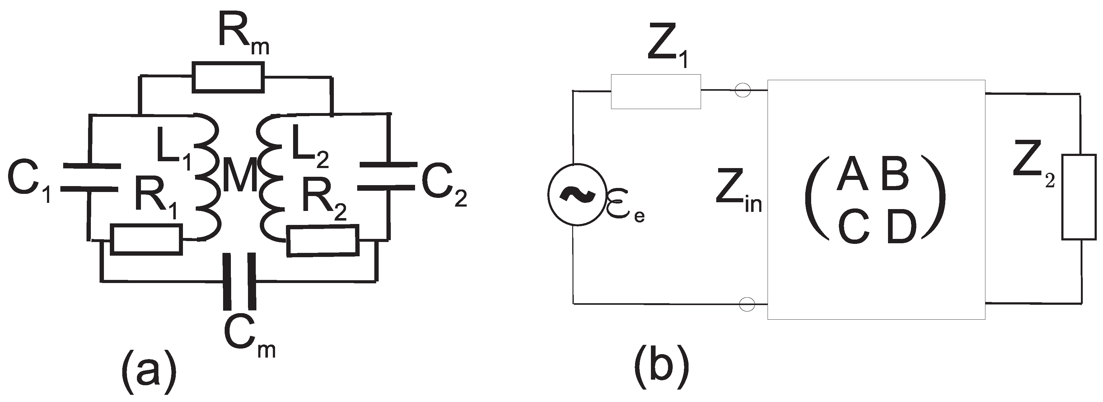
The question of why the dipole-dipole interaction gives the same result as the model of inductive coupling is answered involving the theory of microwave filters [26]. This theory gives the general method for calculating the eigenfrequencies of generally-coupled circuits; when they are connected through the mutual capacitance, resistance and inductance. The general scheme of two arbitrarily-coupled series circuits $Z_1$ and $Z_2$ is shown in Figure 3. The arbitrary connectors of two circuits can be described by an ABCDmatrix of a two-port network. The eigenfrequencies of this system are analyzed in [26] through the elements of the ABCD matrix. If the coupling is reciprocal and symmetric, as is shown in Figure 3a, we have $A=D$ and $A^2-BC=1$. Further, in the special case of the exact resonance $L_1{C}_1=L_2{C}_2$, symmetric coupling corresponds to $A=0$ [26], and the two-port circuit shown in Figure 3b represents the so-called impedance inverter. Then, the application of the ABCD matrix to the load $Z_2$ gives $Z_{\mathrm{in}}=-C^2/Z_2$ for the input impedance of the loaded two-port network. The coupling may comprise all inductive, capacitive or resistive components. For resistive, capacitive, inductive or mixed coupling $C=jK$, where K, called the dimensional coupling parameter, is a real value proportional to $1/\omega$ [26]. In all of these cases, the dispersion equation of the equivalent circuit is $Z_1+Z_{\mathrm{in}}=0$ and takes the form $Z_1{Z}_2=K^2$.

Figure 3. (a) Symmetric coupling of two circuits. (b) An equivalent scheme of our system represented via the impedance inverter ($A=D=0$, $B=-1/C=-jK$, $K>0$).

Figure 3. (a) Symmetric coupling of two circuits. (b) An equivalent scheme of our system represented via the impedance inverter ($A=D=0$, $B=-1/C=-jK$, $K>0$).

After substitutions Equation (4) and the result for K from [23], one may see that the analogy with two different pendulums coupled by the spring does not hold. The model based on the electric near-field coupling of two dipole scatterers [23] yields to the elastic model of [18]. Really, the input impedance $Z_{\mathrm{in}}$, denoted as $Z_m$, was found in [23] in the form $Z_m={\left(\eta N\right)}^2/Z_2$, where N is given by Equation (7). Then, the dimensional coupling parameter is equal to $K=\eta N\equiv l_1{l}_2{A}_{ee}/\omega$. Then, the eigenfrequencies are determined by the parameter ${\kappa }^{\prime }=K\left({\omega }_0\right)/\sqrt{K_1{K}_2}$, where $K_{1,2}=\sqrt{L_{1,2}/C_{1,2}}$ [26]. It is easy to see that ${\kappa }^{\prime }=\kappa \equiv q/{\omega }_0={\omega }_R/{\omega }_0$.

At this point, three models of mutual coupling meet one another. The model of elastic coupling of elastic oscillators [18], that of the general $RLC$ coupling of two circuits (see Figure 3a and [26]) and our model [23] give the same dispersion equation. There are two reasons of this coincidence: the symmetry of the dipole-dipole interaction and the exact resonance we have assumed. These two conditions make the resistive, inductive and capacitive coupling non-distinguished via the coupling parameter K and, therefore, via the dispersion equation.

To conclude this subsection let us notice that the Equation (2) is approximate, and in [26] and similar handbooks, the exact solution is also absent. We have not found an exact solution in the literature and obtained it using the standard Ferrari scheme for equations of fourth order:

$${\omega }_{\pm }={\omega }_0\sqrt{1+{\Phi }^2}-j\frac{{\gamma }_1+{\gamma }_2}{4}\pm$$

$$\sqrt{{\omega }_R^2-{\left(\frac{{\gamma }_1-{\gamma }_2}{4}\right)}^2+{\left(\frac{{\omega }_R^2+{\gamma }_1{\gamma }_2}{4{\omega }_0}\right)}^2+j\frac{{\gamma }_1+{\gamma }_2}{4}\Phi }$$

(13)

where:

$$\Phi =\sqrt{-{\left(\frac{{\gamma }_1-{\gamma }_2}{4}\right)}^2+{\left(\frac{{\omega }_R^2+{\gamma }_1{\gamma }_2}{4{\omega }_0}\right)}^2}$$

It is easy to check that the substitution of this solution exactly equates the left-hand side of Equation (12) to zero. Usually, in plasmon-enhanced fluorescence, decay rates ${\gamma }_1$ and ${\gamma }_2$ are noticeably different, and ${\gamma }_2\gg {\gamma }_1$. Then, in the weak mutual coupling (WMC) regime (defined by the condition ${\omega }_R\ll {\gamma }_2$), $\Phi \approx j({\gamma }_2-{\gamma }_1)/4$ and ${\omega }_R^2\ll {({\gamma }_2-{\gamma }_1)}^2/16$. In this case, the difference between two roots in Equation (13) vanishes, and ${\omega }_{\pm }\approx {\omega }_0-j{\gamma }_2/4$. This clearly shows that the previously known Equation (2) is not relevant, since it does not explain the regime when the two roots of the dispersion Equation coincide in the presence of noticeable decay. This regime, when the fluorescence spectrum of the QE is not distorted by the NA, whereas the decay rate of the system grows due to the presence of the NA, is well known. This is the Purcell effect under weak mutual coupling. In the strong mutual coupling regime (SMC), defined by inequality ${\omega }_R\gg {\gamma }_2$, Equation (3) holds for both Equations (2) and (13).

These observation allow us to conclude that Equation (2) is less relevant than Equation (13) and needs to be replaced. However, we will see below that in between the regimes of WMC and SMC, there is a qualitatively different regime, called below intermediate mutual coupling. For this case, the analysis of the fluorescence spectra based on the solution of the dispersion equation is not very relevant. There is another way to calculate these spectra, which is applicable for all regimes. This way is the evaluation of the dipole moment of the system.

2.4. Rabi Frequency in Quantum Optics

Effective dipole length $l_1$ and electric capacitance $C_1$ seem to be rather artificial values for a QE. However, they have clear physical meaning as parameters of the Lorentz model of a quantum object considered as a scatterer in the external field [4]. In accordance with this model, the dynamic polarizability of the two-level quantum object is the single-resonance Lorentzian function:

$$\alpha ={\alpha }_0{\left(1-\frac{{\omega }^2}{{\omega }_0^2}+j\frac{\omega \gamma }{{\omega }_0^2}\right)}^{-1}$$

(14)

The static polarizability ${\alpha }_0$ of any dipole scatterer is obviously expressed through its effective capacitance and dipole length (see, e.g., [23]) ${\alpha }_0=C{l}^2$. Therefore, the formula for the Rabi frequency ${\omega }_R/{\omega }_0=\kappa =\sqrt{C_1{C}_2}{l}_1{l}_2{A}_{ee}$ can be also written in the form:

$${\omega }_R\equiv q={\omega }_0\kappa ={\omega }_0{A}_{ee}\sqrt{{\alpha }_{01}{\alpha }_{02}}$$

(15)

Here, the static polarizability ${\alpha }_{01}$ of the two-level QE can be expressed through the absolute value of the transition dipole moment d [4]:

$${\alpha }_{01}=\frac{2d^2}{\hslash {\omega }_0}$$

(16)

and finally, Equation (15) becomes:

$${\omega }_R=d{A}_{ee}\sqrt{\frac{{\omega }_0{\alpha }_{02}}{2\hslash }}$$

(17)

Let us see how this classical model stands the comparison with the known results of a semiclassical model of plasmon-enhanced fluorescence [13,14,16]. In accordance with this theory, the linear SMC regime represents the Rabi oscillations of the emission. In our case of exact resonance, the difference between the upper frequency ${\omega }_{+}$ and lower frequency ${\omega }_{-}$ of the hybrid state equals the doubled Rabi constant:

$$\Delta \omega =2{\omega }_R=2\frac{\mathbf{d}·{\mathbf{E}}_{21}^V}{\hslash }$$

(18)

Value ${\omega }_R$ formally coincides with the standard formula for Rabi oscillations of a QE impinged by an incident wave [4]. However, in the present case, ${\mathbf{E}}_{21}^V$ is the so-called vacuum field of the NA [13]. This vacuum field corresponds to the resonant eigenmode of the localized surface plasmon in the NA. The eigenmodes of the surface plasmon can be obtained by quantingthe classical electromagnetic field of the NA. In the simplest case, when Object 2 is a silver or golden nanosphere of radius $a\ll \lambda$ (λ is the wavelength in the host material), these eigenmodes correspond to equations ${\epsilon }_m\left(\omega \right)=-(n+1){\epsilon }_r/n$, $n=1,2,\dots$ (see, e.g., [28]) with the substitution of the analytical (e.g., Drude’s) model for the relative permittivity of the metal ${\epsilon }_m\left(\omega \right)$, where the imaginary part is neglected. The dipole mode of the sphere corresponds to $n=1$, i.e., ${\epsilon }_m\left(\omega \right)=-2{\epsilon }_r$. At frequency ${\omega }_0$, corresponding to this condition, the quant of the plasmon electric field reads as [28]:

$$E_{10}=\sqrt{\frac{4\pi \hslash {\omega }_0}{3a}}$$

(19)

The quant $E_{10}$ determines the dipole moment of the lowest eigenmode of a plasmonic nanosphere [28]:

$$d_2^V=\sqrt{4\pi \hslash {\omega }_0{\epsilon }_0{\epsilon }_r{a}^3}$$

(20)

The vacuum field ${\mathbf{E}}_{21}^V$ is that produced by the this dipole moment at a distance r from the sphere center. For the geometry with collinear dipole moments of the QE and the NA (as in [17]), we have:

$$E_{21}^V=\sqrt{\frac{2\hslash {\omega }_0{a}^3}{\pi {\epsilon }_0{\epsilon }_r}}\frac{1}{r^3}$$

(21)

Substituting Equation (21) into Equation (18), we obtain for the Rabi constant:

$${\omega }_R=\frac{d}{r^3}\sqrt{\frac{2a^3{\omega }_0}{\hslash \pi {\epsilon }_0{\epsilon }_r}}$$

(22)

It is evident that Equation (22) is equivalent to previously-derived Relation Equation (17) after two following substitutions into Equation (17): Equation (8) for $A_{ee}$ and ${\alpha }_{02}=4\pi {\epsilon }_0{\epsilon }_r{a}^3$ for the static limit value of the polarizability of a metal sphere. This value is common for all metals with the Drude-type dispersion [27].

Therefore, our classical circuit model, which borrows from quantum optics only the static polarizability of the two-level system, exactly describes the Rabi splitting in the nanosystem. We have proven this coincidence for the special case of spherical NA; however, we believe that our model remains applicable to any NA of the dipole type, e.g., to that sketched in Figure 1.

2.5. Fluorescence Spectra beyond the WMC Approximation

Now, using our dipole-dipole model and the approach of weak perturbations, let us find the dipole moments of Objects 1 and 2 at arbitrary frequency ω. The sum of these dipole moments determines the radiated power at this frequency. In order to solve the problem within the framework of the classical model, let us apply the weak perturbation method. In the zero approximation, there is no feedback, and the spectrum of the emission is unperturbed. This field spectrum has a Lorentzian shape [4], i.e., the spectrum of its dipole moment of QE in the zero approximation can be modeled using the Lorentzian spectral function $S_1\left(\omega \right)$ [11]:

$$d_1^{\left(0\right)}\left(\omega \right)=d_{10}{S}_1\left(\omega \right),S_1\left(\omega \right)\equiv {\left(1-\frac{{\omega }^2}{{\omega }_0^2}+j\frac{\omega {\gamma }_1}{{\omega }_0^2}\right)}^{-1}$$

(23)

Here, the parameter $d_{10}$ can be found from the condition that at the resonance, the classical dipole moment $d_1\left({\omega }_0\right)$ is two-fold of the transition dipole moment $d_1\left({\omega }_0\right)=2d$ [4]. Then, $d_{10}=2jd{\gamma }_1/{\omega }_0$. The field produced at the center of Object 2 in the zero approximation equals:

$$E_{12}\left(\omega \right)=\frac{2j{\gamma }_{1}d{A}_{ee}}{{\omega }_0}{S}_1\left(\omega \right)$$

(24)

In the first approximation, this field induces in the NA the dipole moment $d_2^{\left(1\right)}\left(\omega \right)={\alpha }_2\left(\omega \right)E_{12}\left(\omega \right)$, where ${\alpha }_2$ is proportional to the Lorentzian function $S_2\left(\omega \right)$ [23]:

$${\alpha }_2={\alpha }_{02}{S}_2\left(\omega \right),S_2\left(\omega \right)\equiv {\left(1-\frac{{\omega }^2}{{\omega }_0^2}+j\frac{\omega {\gamma }_2}{{\omega }_0^2}\right)}^{-1}$$

(25)

This dipole moment, in turn, induces in the QE an additional dipole moment, which in the first-approximation equals $d_{\mathrm{1ind}}^{\left(1\right)}\left(\omega \right)={\alpha }_1\left(\omega \right)E_{21}\left(\omega \right)$. Here, $E_{21}\left(\omega \right)=d_2^{\left(1\right)}\left(\omega \right)A_{ee}$ is the field produced at the center of the QE by the dipole moments $d_2^{\left(1\right)}\left(\omega \right)$, and the polarizability of the QE ${\alpha }_1$ is given by Equation (14), which can be rewritten as:

$${\alpha }_1={\alpha }_{01}{S}_1\left(\omega \right),{\alpha }_{01}=\frac{2d^2}{\hslash {\omega }_0}$$

(26)

If we restrict the analysis by the first approximation, we have for the total dipole moment $d_{\mathrm{tot}}=d_1^{\left(0\right)}+d_{\mathrm{1ind}}^{\left(1\right)}+d_2^{\left(1\right)}$, i.e.:

$$d_{\mathrm{tot}}=d_1^{\left(0\right)}{F}_d,F_d\equiv 1+{\alpha }_2{A}_{ee}(1+{\alpha }_1{A}_{ee})$$

(27)

The radiated power is proportional to $|d_{\mathrm{tot}}{|}^2$:

$$P_{\mathrm{rad}}=\frac{|d_1^{\left(0\right)}{|}^2{\left|F_d\right|}^2}{12\pi {\epsilon }_0{c}^3}$$

(28)

The birefringence of the radiation spectrum, which corresponds to two different solutions of the dispersion Equation (13), arises also in Equations (27) and (28). It results from the multiplication of two Lorentzian functions in the term ${\alpha }_1{\alpha }_2{A}_{ee}^2={\alpha }_{01}{\alpha }_{02}{A}_{ee}^2{S}_1\left(\omega \right)S_2\left(\omega \right)$ in the last term.

In the regime of WMC, this term is negligible, and Equation (27) should give the non-distorted spectrum. Let us compare the result of Equation (27) with that obtained for the regime of WMC in [23] through the analysis of the radiation resistance. Equation (30) of [23] for the Purcell factor has the form:

$$F_P=1-\mathrm{Im}\left({\alpha }_2\right)\frac{6\pi c^2}{{\omega }^3\eta }{A}_{ee}^2.$$

(29)

In the case of WMC, ${\alpha }_1{A}_{ee}\ll 1$. In this case, Equation (27) simplifies to $F_d\approx 1+{\alpha }_2{A}_{ee}$, and for the modification of the fluorescence spectrum, we have:

$$|F_d{|}^2=1+{\left|{\alpha }_2\right|}^2{A}_{ee}^2+2\mathrm{Re}\left({\alpha }_2\right)A_{ee}.$$

(30)

Equations (29) and (30) meet one another when in both QE and NA radiative losses dominate over the dissipation. The expression Equation (30) obtained in [23] was based on this assumption. Then, the parameters ${\gamma }_{1,2}$ in Equations (23) and (25) can be approximately identified with radiative losses. To identify ${\gamma }_{1,2}$ with radiative losses is to equate $\mathrm{Im}(1/{\alpha }_{1,2})$ to ${\omega }^3/6\pi {\epsilon }_0{c}^3$ [23]. Here, for simplicity, we put ${\epsilon }_r=1$. This results in the relation:

$${\gamma }_{1,2}=\left(\frac{{\omega }_0^2{\alpha }_{01,02}}{6\pi {\epsilon }_0{c}^3}\right){\omega }^2$$

(31)

Applying this relation to the NA, we obtain:

$$\mathrm{Im}\left({\alpha }_2\right)\equiv -|{\alpha }_2{|}^2\mathrm{Im}\left(\frac{1}{{\alpha }_2}\right)=-{\left|{\alpha }_2\right|}^2\frac{{\omega }^3\eta }{6\pi c^2}$$

and Equation (29) becomes:

$$F_P=1+{\left|{\alpha }_2\right|}^2{A}_{ee}^2$$

(32)

In the resonance band, $|{\alpha }_2|A_{ee}\gg 1$ and the second term in Equation (27) dominates, as well as in Equation (32). Therefore, for the frequencies within the resonance band, $|F_d{|}^2\approx {\left|{\alpha }_2\right|}^2{A}_{ee}^2\approx F_P$. Beyond the resonance band, both Equations (27) and (29) give $|F_d{|}^2\approx F_P\approx 1$. This approximate equivalence of the present result with that of [23] is an important check.

Notice, that the analysis of [23], resulting in Equations (29) and (32), corresponded to the zero approximation of the weak perturbation method. Equation (27) corresponds to the first approximation. However, the perturbation method for two interacting dipoles is converging. Continuing the procedure, we come to a geometric progression for $F_d$:

$$F_d=1+{\alpha }_2{A}_{ee}(1+{\alpha }_1{A}_{ee})\sum _{n=0}^{\infty }{\left({\alpha }_1{\alpha }_2{A}_{ee}^2\right)}^n$$

which is easily calculated and results in:

$$F_d=\frac{1+{\alpha }_2{A}_{ee}}{1-{\alpha }_1{\alpha }_2{A}_{ee}^2}$$

(33)

Here, ${\alpha }_1$ and ${\alpha }_2$ are given by Equations (25), (26) and (31). Equation (33) finalizes our circuit model, which is now extended beyond the approximation of WMC.

Notice that the expression Equation (33) does not describe the Rabi splitting. The product ${\alpha }_1{\alpha }_2$ in the denominator of Equation (33) due to the relative smallness of ${\alpha }_1$ gives only a distortion of $F_d$ from the Lorentzian spectrum. This distortion is not symmetric with respect to the central frequency ${\omega }_0$. The Rabi splitting occurs because in Equation (28), both factors $d_1^{\left(0\right)}$ given by Equation (23) and $F_d$ given by Equation (33) possess resonant frequency dispersion with the same resonant frequency.

Note that in the static limit when ${\alpha }_1{\alpha }_2$ are real values, the denominator in the right-hand side of Equation (33) does not experience singularity. On the contrary, it nearly equals unity, since ${\alpha }_{01}{\alpha }_{02}{A}_{ee}^2\ll 1$. This is so because r entering $A_{ee}$ is larger than $a+b$. Though $A_{ee}$ is very large, it cannot cover the smallness of ${\alpha }_{01}$. For the frequency of the individual resonance $\omega ={\omega }_0$, the product ${\alpha }_1\left({\omega }_0\right){\alpha }_2\left({\omega }_0\right)$ is negative. In the case of WMC, this value is negligibly small, but in the case of SMC, it is comparable with $-1$ and gives the local minimum, usual the result of the theory of two coupled circuits.

Since we are interested in resonant effects, calculating $F_d$ in practical cases, we may use the standard approximation of frequency-independent decay parameters, putting in Equations (25) and (26):

$${\gamma }_{1,2}\approx \frac{{\omega }_0^4{\alpha }_{01,02}}{6\pi {\epsilon }_0{c}^3}$$

(34)

Quasi-static parameters ${\alpha }_{02}$ and $A_{ee}$, as well as ${\alpha }_{01}=2d^2/\hslash {\omega }_0$ are positive values and are determined by the design of the NA and the location of the QE.

2.6. Express-Analysis of the Fluorescence Spectra

The express-analysis of the fluorescence spectra is done here for the most practically interesting case when ${\gamma }_1\ll {\gamma }_2$ (high-decay NA) [1,5,6,7,8]. We have performed this analysis for the simplest scheme when the NA is a silver or golden nanosphere of radius a and the QE of effective radius b is separated from it by a gap G, substantial enough to prevent tunneling.

The emitter-field coupling and mutual coupling are described by the constants:

$$\chi =d\sqrt{\frac{3{\omega }_0}{8\pi \hslash {\epsilon }_0{b}^3}},{\omega }_R=\frac{d}{r^3}\sqrt{\frac{2a^3{\omega }_0}{\pi \hslash {\epsilon }_0}}$$

(35)

where $r=a+b=G$, whereas from Equation (31) for ${\gamma }_1$ and ${\gamma }_2$, we have:

$${\gamma }_1\approx d^2\frac{{\omega }_0^3}{3\pi \hslash {\epsilon }_0{c}^3},{\gamma }_2\approx \frac{2a^3{\omega }_0^4}{3c^3}$$

(36)

The condition ${\gamma }_1\ll {\gamma }_2$ practically holds when $a>b$ [11].

Since ${\omega }_R$ is always lower than χ, we may share the following regimes depending on ${\omega }_{0}a/c$, $G/b$, $a/b$ and $\chi /{\omega }_0$. For the emitter-field coupling, there are three regimes: (1) weak emitter-field coupling (WEFC), when $\chi <{\gamma }_1$; (2)intermediate emitter-field coupling (IEFC), when ${\gamma }_1<\chi <{\gamma }_2$; and (3) strong emitter-field coupling (SEFC), when $\chi >{\gamma }_2$. For the mutual coupling between QE and NA, there are also three basic regimes: (1) WMC, when ${\omega }_R<\chi <{\gamma }_1$; (2) intermediate mutual coupling (IMC), when ${\gamma }_1<{\omega }_R<{\gamma }_2$; and (3) strong mutual coupling (SMC), when ${\omega }_R>{\gamma }_2$. The peculiarities of the fluorescence are explained via the combination of emitter-field coupling and mutual coupling. In the regime of WMC, one can share four cases:

• WEFC; then, for any relative gap $G/b$ between QE and NA, there is no noticeable enhancement of the emission: $F_d\left({\omega }_0\right)\sim 1$.
• IEFC, large gap $G\gg a$, when $F_d\left({\omega }_0\right)\sim 1$.
• IEFC, intermediate gap $b<G<a$, when the noticeable enhancement of the emission arises: $F_d\left({\omega }_0\right)\gg 1$; however, the fluorescence spectrum remains Lorentzian.
• SEFC; the combination of SEFC and WMC is possible only when $G\gg a$; then $F_d\left({\omega }_0\right)\sim 1$.

Therefore, in the WMC regime, the noticeable Purcell effect (without distortions of the spectrum) holds only for QE with IEFC.

The regime of IMC cannot be realized in the case of WEFC. For this regime, the two following cases can be shared:

• IEFC: This combination is possible when $b<G<a$. Then, the strong enhancement of the emission arises: $F_d\left({\omega }_0\right)\gg 1$. Furthermore, the fluorescence spectrum is noticeably distorted compared to the usual Lorentzian line.
• SEFC: This is possible when $G\sim a$. Then, the strong enhancement of the emission arises: $F_d\left({\omega }_0\right)\gg 1$. Furthermore, the fluorescence spectrum is distorted strongly: the Rabi splitting arises.

Therefore, the regime of IMC is characterized by the strong Purcell effect, which is combined with the distortion of the spectrum. For QE with SEFC, this distortion corresponds to the Rabi oscillations.

The regime of SMC can be implemented only together with SEFC when the gap is small $G\ll a$. In this case, $F_d\left({\omega }_0\right)\ll 1$. This regime deserves our special attention, because here, our classical model explains the fluorescence quenching.

When two identical oscillators are strongly coupled, the individual resonance splits into two hybrid resonances whose magnitude is slightly lower than that of the individual one. This is so in the case of the inductive coupling. Then, the ratio of the magnitude of the hybridized resonances to that of the individual one is equal ${\gamma }_{1,2}/4{\omega }_R$. This ratio becomes smaller in the case of the dipole coupling, which is our case. In the case of SMC, the hybrid frequencies are given by Equation (3) with $q\equiv {\omega }_R$, described by Equation (15). Further, $S_{1,2}\left({\omega }_{pm}\right)\approx \pm {\kappa }^{-1}$ in Equations (25), (26) and (31), and ${\alpha }_2\left({\omega }_{pm}\right)\approx {\alpha }_{02}{\omega }_0/{\omega }_R$. Since $\kappa \gg {\gamma }_2/{\omega }_0$, the value ${\alpha }_2\left({\omega }_{pm}\right)$ is much smaller than ${\alpha }_2\left({\omega }_0\right)={\alpha }_{02}{\omega }_0/{\gamma }_2$. Moreover, the factor ${\omega }_0^3{r}^3/c^3$ in the product ${\alpha }_2\left({\omega }_{pm}\right)A_{ee}$ cancels out, and this value turns out to be smaller than unity. Therefore, Equation (33) gives $F_d\left({\omega }_{\pm }\right)\approx 1$. The emitted power at these frequencies $P_{\mathrm{rad}}\left({\omega }_{pm}\right)$ is determined by the product $|d_1^{\left(0\right)}\left({\omega }_{pm}\right){|}^2{\left|F_d\left({\omega }_{pm}\right)\right|}^2$ in the right-hand side of Equation (28), where $d_1^{\left(0\right)}$ at frequencies ${\omega }_{pm}$ is far beyond the resonance band of the QE and, therefore, is very small. In accordance with Equation (23), $d_1^{\left(0\right)}\left({\omega }_{pm}\right)$ is equal to $2d{\gamma }_1/{\omega }_R$, i.e., is ${\omega }_R/{\gamma }_1\gg 1$ times smaller than $d_1^{\left(0\right)}\left({\omega }_0\right)=2d$. Since in the case of SMC, ${\omega }_R>{\gamma }_2\gg {\gamma }_1$, the ratio ${\omega }_R/{\gamma }_1$ is huge, and $|d_1^{\left(0\right)}\left({\omega }_{pm}\right){|}^2$ is negligible compared to $|d_1^{\left(0\right)}\left({\omega }_0\right){|}^2$. Since $|F_d\left({\omega }_{\pm }\right)|$ is the value of the order of unity, $P_{\mathrm{rad}}\left({\omega }_{\pm }\right)$ turns out to be much smaller than the power emitted by a single QE.

Now, consider the radiated power at the initial emission frequency ${\omega }_0$. The product ${\alpha }_1{\alpha }_2$ entering our Equation (33) at frequency ${\omega }_0$ is negative and equal to $-{\omega }_0^2{\alpha }_{01}{\alpha }_{02}/{\gamma }_1{\gamma }_2$. Expression $1-{\alpha }_1{\alpha }_2{A}_{ee}^2$ is equal to $1+A_{ee}^2{\omega }_0^2{\alpha }_{01}{\alpha }_{02}/{\gamma }_1{\gamma }_2$. In the regime of SMC in spite of the smallness of the value ${\alpha }_{01}$, the product $A_{ee}^2{\omega }_0^2{\alpha }_{01}{\alpha }_{02}/{\gamma }_1{\gamma }_2$ is very large, which makes $|F_d\left({\omega }_0\right)|\ll 1$. Analyzing the derivative of $|F_d\left(\omega \right)|$, it is possible to show that in the case of SMC, this derivative vanishes and $|F_d\left(\omega \right)|$ has the local minimum at ${\omega }_0$. The product $|d_1^{\left(0\right)}{F}_d|$ entering Equation (28) also has the local minimum at this frequency.

Therefore, the radiated power $P_{\mathrm{rad}}$ in the case of SMC at all three characteristic frequencies—${\omega }_0$ and ${\omega }_{\pm }$—turned out to be much smaller than that radiated at the emission frequency ${\omega }_0$ by the isolated QE. This implies the suppression of the radiation over the whole spectrum. However, the spectrum shape keeps that of Rabi oscillations, with maxima at ${\omega }_{\pm }$ and minimum at ${\omega }_0$. Therefore, the regime of SMC can be called weakly radiative or even non-radiative Rabi oscillations.

It can be asserted that this effect is the same as that in the available literature that is treated as fluorescence quenching (see, e.g., [3,5,6,7,8,9,10]). In the literature, the suppression of fluorescence has been analyzed using either a purely quantum model (e.g., [9]) or a semiclassical model (e.g., [10]). The quantum model treats the fluorescence quenching as a threshold effect and relates it to the tunneling. However, in [10], it was shown that this effect exists for any distance r and corresponds to the non-radiative power exchange between the QE and NA. The quenching effect competes with the direct Purcell effect, which corresponds to the radiative power exchange [10]. The Purcell factor and the quenching factor both decrease versus r with the same rate $1/r^6$; thus, there is an optimal distance (a few nm) where the fluorescence enhancement is maximal. However, for QE with WEFC, the quenching (as well as the strong Purcell enhancement) is not observed.

These literature data are in line with the results of our circuit model. Really, the Purcell factor described by Equation (32) is nearly proportional to $A_{ee}^2=1/4{\pi }^2{\epsilon }_0^2{r}^6$. The damping factor being proportional to ${\omega }_R^2$ is also proportional to $1/r^6$ in accordance with Equation (35). Since the value $|d_1^{\left(0\right)}{|}^2$ in Equation (28) at ${\omega }_{\pm }$ is equal $4d^2{\gamma }_1^2/{\omega }_R^2$, Equations (28) and (33) allow one to find an optimal distance r (as a deal between damping and Purcell factors) for the given d analytically. It is easy to see that the optimal value of the gap G is within the interval $[b,a]$. For $G<b$, the coupling becomes strong, and the hybridization shifts the two resonance frequencies from the band where the mutual coupling has the dominating resistive component [23]. The mutual coupling becomes reactive, and more energy is stored in the QE due to the presence of the NA. These results of our model qualitatively coincide with the conclusions of [10].

However, a comment should be made here. For QE with SEFC, the contest of the enhancement and quenching should be considered together with the modification of the spectrum. If we take into account that the shift of the resonance frequencies from the individual resonance depends on the distance r, the Purcell factor described by Equation (33) becomes not obviously monotonous versus r. It is monotonous only in Equation (32), which corresponds to the regimes of WEFC and IEFC. In these cases, the fluorescence spectrum is modified not very strongly, and $|F_d{|}^2\left(\omega \right)\approx F_P\left(\omega \right)$. In the case of SEFC, the strong modification of the spectrum occurs for the same system if we vary the distance r. For small r, SEFC implies SMC (the mutual coupling becomes strong), and $|F_d{|}^2$ at frequencies ${\omega }_{\pm }$ becomes of the order of unity, whereas at ${\omega }_0$$|F_d{|}^2\ll 1$. Therefore the enhancement over the whole spectrum is also not monotonous versus r.

3. Results and Discussion

3.1. Numerical Examples

In order to validate the theory on an explicit example, we have considered a quantum dot whose fluorescence is enhanced by a golden sphere of diameter $2a=24.5$ nm located at a distance $G=3$ nm from one another. Exact simulations for this case were done in [32] using the semi-classical model. The Drude-like model for the complex permittivity of gold corresponds to [33]. The radiating system is located in the liquid host ${\epsilon }_r=2.89$. The single quantum dot emits at ${\lambda }_{01}=535$ nm. This wavelength nearly coincides with the plasmon resonance of the metal sphere in the liquid, which holds at ${\lambda }_{02}=520$ nm.

Figure 4. Fluorescence spectrum of a quantum dot coupled to a golden nanosphere normalized to that of the single quantum dot. Thin line: zero-order model [23]. Dashed line: exact simulations of the semiclassical model [32]. Thick line: our general Formula (33).

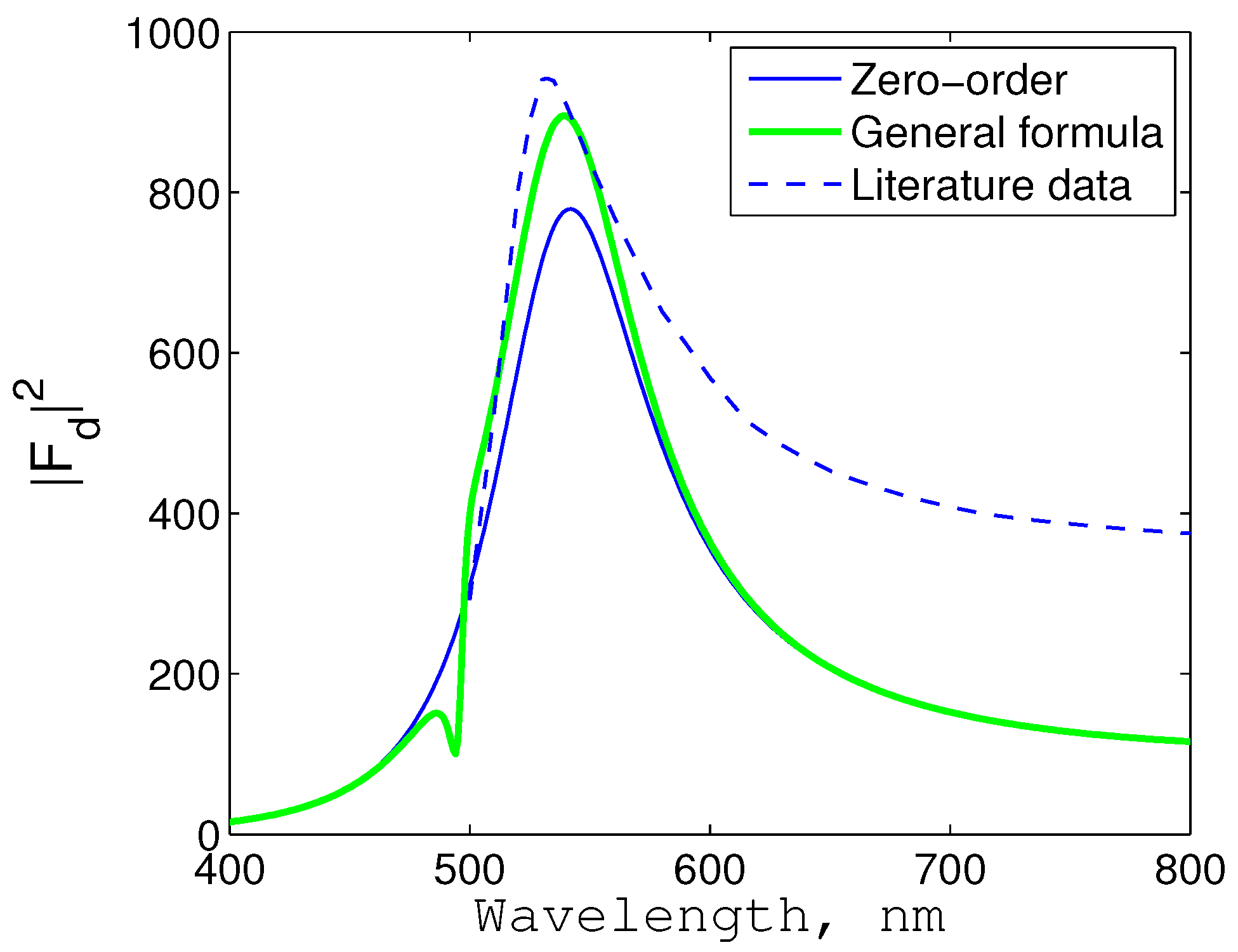
Figure 4. Fluorescence spectrum of a quantum dot coupled to a golden nanosphere normalized to that of the single quantum dot. Thin line: zero-order model [23]. Dashed line: exact simulations of the semiclassical model [32]. Thick line: our general Formula (33).

The fluorescence spectrum calculated in [32] was normalized to the radiated power of the single QE. In fact, in Figure 1 of [32], the authors show the radiative and non-radiative parts of the Purcell factor (they call them the normalized radiative and non-radiative decay rates) in a broad range of wavelength (500–900 nm). The sum of these two factors in accordance with [23] gives the total frequency-dependent Purcell factor, i.e., in our notations representing the value $|F_d{|}^2$. These numerical data were compared with $|F_d{|}^2$ calculated using the zero-order approximation Equation (32) and using the final Equation (33). The polarizability ${\alpha }_2$ of the metal nanosphere was calculated taking into account the dissipation Equation (like in [23]). The results are shown in Figure 4. For the decay factor of the quantum dot, we used the lossless approximation Equation (31).

Within the plasmon resonance band, the zero-order model represented by a thin solid curve is in rather good agreement with the exact calculations (dashed curve). The error becomes more significant beyond the resonance. Here, we concentrate on the high-frequency edge of the resonance band where the zero-order model predicts the Lorentzian shape for the spectrum, whereas the dashed curve clearly has a huge non-Lorentzian slope. The comparison with the result of Equation (33) shows the reason for this strong non-symmetry of the spectral line. Extending the range of wavelengths to 400–500 nm (in [32], calculations are done for 500–900 nm), we can see the typical feature of the Fano resonance with the dip at 500 nm. Clearly, the inexact coincidence of the plasmon resonance and the emission frequency together with the difference in decay rates obviously result in this type of resonance. In general, the behavior of the thick curve in the resonance band fits the exact data much better: the error for the maximal value of $|F_d{|}^2$ reduces from 12% (thin Curve 1) to 4% (thick curve).

Calculating parameters ${\gamma }_{1,2}$ and ${\omega }_R$ with the use of Equation (35), we saw that this system in our terminology corresponds to the case of IMC. This is the most difficult case, when the hybridization does not result in the Rabi splitting, but results in the strong distortion of the spectral shape compared to the usual Lorentzian line. This distortion is the Fano resonance.

Notice that the model developed in this paper does not imply obviously the condition of the exact resonance. This condition was used only to simplify the comparison of our model with previous analytical models. In fact, our circuit model allows (at least approximately) predictions of fluorescence spectra in the practical case when the resonance of the nanosystem is approximate. Our Equation (33) does not require the exact resonance. The polarizabilities of the quantum dot ${\alpha }_1$ and that of the NA ${\alpha }_2$ may be calculated using Equations (25) and (26) also beyond the exact resonance. We may put different resonant frequencies ${\omega }_{01}$ and ${\omega }_{02}$ into Equations (25) and (26), and nothing will change in our model. The relative difference $({\lambda }_{01}-{\lambda }_{02})/({\lambda }_{01}+{\lambda }_{02})=0.028$ is sufficient to produce the noticeable Fano resonance: a narrow spectral hole near the rather broad maximum. Of course, the Lorentzian line results from the zero-order approximation (the same Equation (33) with the substitution ${\alpha }_1=0$).

We do not know exactly the reasons for the disagreement between the exact dashed curve and our theoretical thick curve at wavelengths 600–800 nm where the quasi-static dipole model is expected to work better than in the resonance band. Most probably, this disagreement is related to dissipative losses in the quantum dot, which were fully neglected in our calculations. These losses may enlarge the low-frequency part of the resonance band. Furthermore, the value d, which determines the static polarizability ${\alpha }_{01}$ of the QE, is not exactly known, since it is not given in [32]. We found this d using a fitting procedure. The thick curve in Figure 4 corresponds to $d=14.5$ D, when the numerical deviation from the dashed curve is minimal over the resonance band $\lambda =$ 500–600 nm. Slightly larger values of d correspond to a much larger maximum of $|F_d{|}^2$; slightly smaller values correspond to a much broader resonance band. This value $d=14.5$ D for a two-level nanocrystal quantum dot is realistic. In accordance with [34], the estimation of the transition dipole moment is as follows: $d=1.21eb{\epsilon }_r/(2{\epsilon }_r+{\epsilon }_{QD})$, where e is the electron charge and ${\epsilon }_{QD}$ is the relative permittivity of the quantum dot semiconductor at the emission frequency. This formula gives for the InSb quantum dot the value $d=25.1$ D, i.e., the value of the same order of magnitude as that given by our numerical fitting.

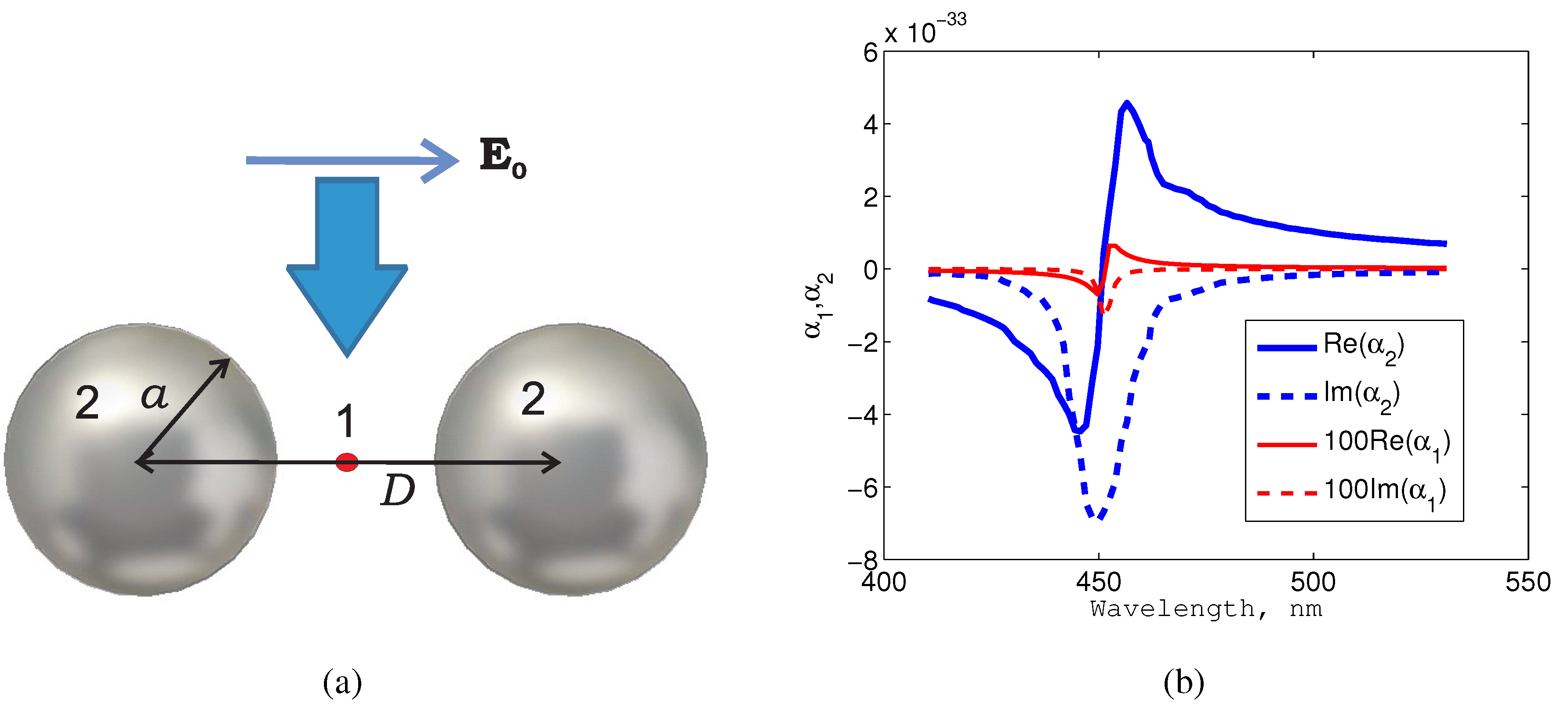
In [16], one notices that the Fano resonance occurs in the extinction spectra, even if the resonances of the QE and NA coincide. The strong asymmetry of the frequency dependence inherent to the Fano resonance becomes possible because the shape of the Lorentzian spectral line is not perfectly symmetric with respect to ${\omega }_0$. Therefore, even for the exact resonance, the Fano spectral hole may result from the interference of the very tiny resonance band of a quantum dot compared to that of the plasmon resonance of an NA. The condition of the Fano resonance in this case is a sufficient value of the resonant polarizability of the QE. In [16], one calculates the extinction cross-section of the structure depicted in Figure 5a. A quantum dot located at the center of a plasmonic dimer of Ag nanospheres is illuminated symmetrically by a plane wave, whereas the whole nanosystem is placed in the host ${\epsilon }_h=3$. In Figure 3b of [16], the evolution of the extinction cross-section (ECS) is presented when the transition dipole moment d varies from zero to $d=e·B$, where $B=0.7$ nm. In all cases, QE 1 and NA 2 have their individual resonances at the same wavelength $\lambda =$ 450 nm. The complex permittivity of silver is taken from [35].

Figure 5. (a) Sketch of the simulated nanosystem, where $D=22$ nm, $a=7$ nm; (b) complex polarizabilities of Elements 1 and 2 illuminated separately for the case $d/e=0.3$ nm. Polarizability ${\alpha }_1$ is calculated analytically, and ${\alpha }_2$ is simulated numerically using the CST software.

Figure 5. (a) Sketch of the simulated nanosystem, where $D=22$ nm, $a=7$ nm; (b) complex polarizabilities of Elements 1 and 2 illuminated separately for the case $d/e=0.3$ nm. Polarizability ${\alpha }_1$ is calculated analytically, and ${\alpha }_2$ is simulated numerically using the CST software.

The spectra of ECS in semiclassical calculations of [16] were normalized to the maxima of these spectrum for every value of d. We have performed similar calculations and compared the evolution of spectra versus d with the numerical data of [16]. Let us consider the single QE 1, with polarizability ${\alpha }_1$ illuminated by a plane wave. Then, its individual dipole moment equals $d_{10}={\alpha }_1{E}_0$. Now, let us illuminate the nanosystem, as is shown in Figure 5a. Then, the total dipole moment of the system $d_{\mathrm{tot}}=d_1+d_2=({\alpha }_1+{\alpha }_2)E_0+{\alpha }_1{E}_{21}+{\alpha }_2{E}_{12}$, where $E_{21}=A_{ee}{d}_1$ and $E_{12}=A_{ee}{d}_2$ are interaction fields expressed through the interaction constant $A_{ee}$. In the case of the dimer, this constant is not so simple to calculate analytically, because the coupling field $E_{12}$ is now produced by two nanospheres, which are additionally mutually coupled with one another. This coupling though basically dipoles is not exactly that of two point dipoles located at their centers. The coupling of silver nanospheres also qualitatively modifies the frequency dependence of the individual polarizability of the dimer compared to that of a single sphere. Therefore, we performed exact numerical simulations of both $A_{ee}$ and ${\alpha }_2$. Using the CST software, we have calculated the dipole moment of the NA 2, integrating its polarization currents, and found the complex value ${\alpha }_2=d_2/E_0$. In the same simulation project, the value $A_{ee}$ was found as $A_{ee}=E_{12}/d_2$, where the field $E_{12}=E_c-E_0$ ($E_c$ is the total electric field at the center of the dimer). The polarizabilities ${\alpha }_1$ for different values of d were found using Equation (26), neglecting the dissipation in the QE. In Figure 5b, we depict ${\alpha }_1$ (analytically calculated) and ${\alpha }_2$ (numerically simulated) for the realistic case $B\equiv d/e=0.3$ nm (then $d=15$ D), which may correspond to a quantum dot of a radius of 2 nm [16]. The resonance band of this QE turns out to be ten-times narrower than that of the NA, and the resonant value of $|{\alpha }_1|$ is lower than that of $|{\alpha }_2|$ by three orders of magnitude. However, we will see below that in combination with the plasmonic dimer, it is enough for the Rabi splitting.

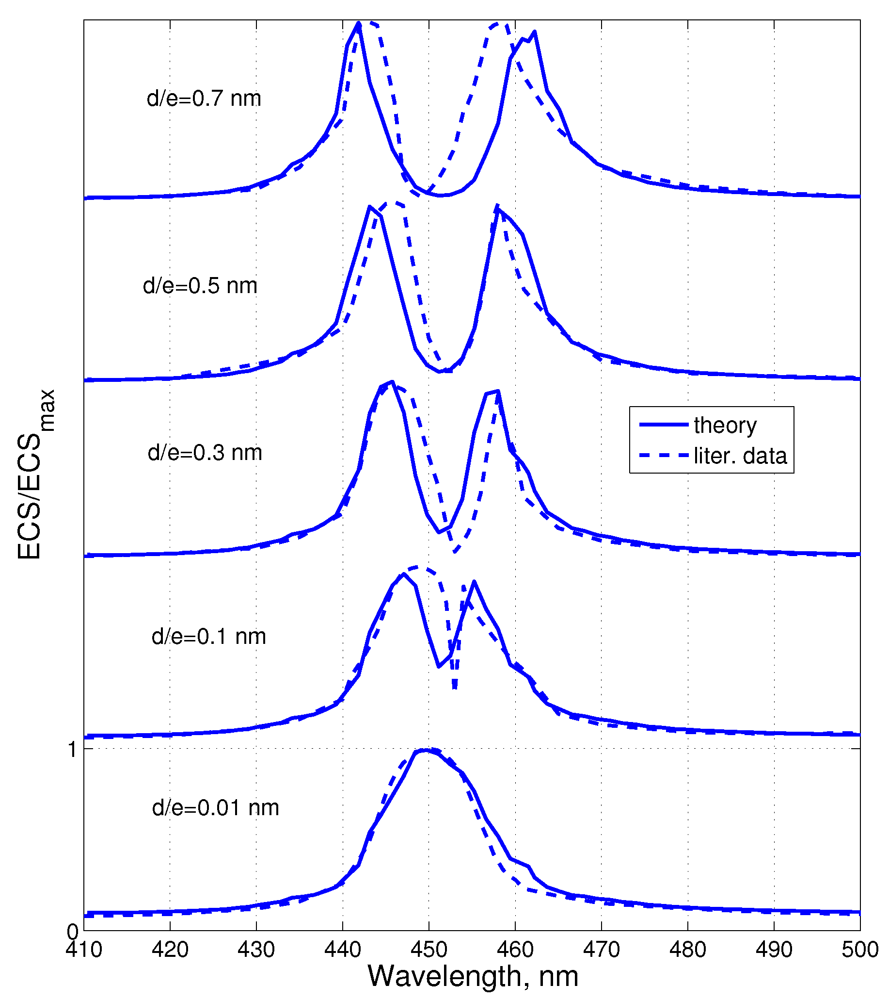
Figure 6. Normalized extinction cross-sections versus wavelength for five values of the transition dipole moment: solid curves: Equation (33); dashed ones: data from [16].

Figure 6. Normalized extinction cross-sections versus wavelength for five values of the transition dipole moment: solid curves: Equation (33); dashed ones: data from [16].

Once we know values ${\alpha }_{1,2}$ and $A_{ee}$, we may find $d_{\mathrm{tot}}={\alpha }_{\mathrm{tot}}{E}_0$ and, applying the same speculations as above, derive ${\alpha }_{\mathrm{tot}}={\alpha }_1{F}_d$, where Equation (33) still holds for $F_d$. This allows us to study the evolution of extinction spectra versus $d=eb$ because (see, e.g., [27]):

$$ECS=-\eta \omega \mathrm{Im}\left({\alpha }_{\mathrm{tot}}\right)=-\eta \omega \mathrm{Im}\left({\alpha }_1{F}_d\right)$$

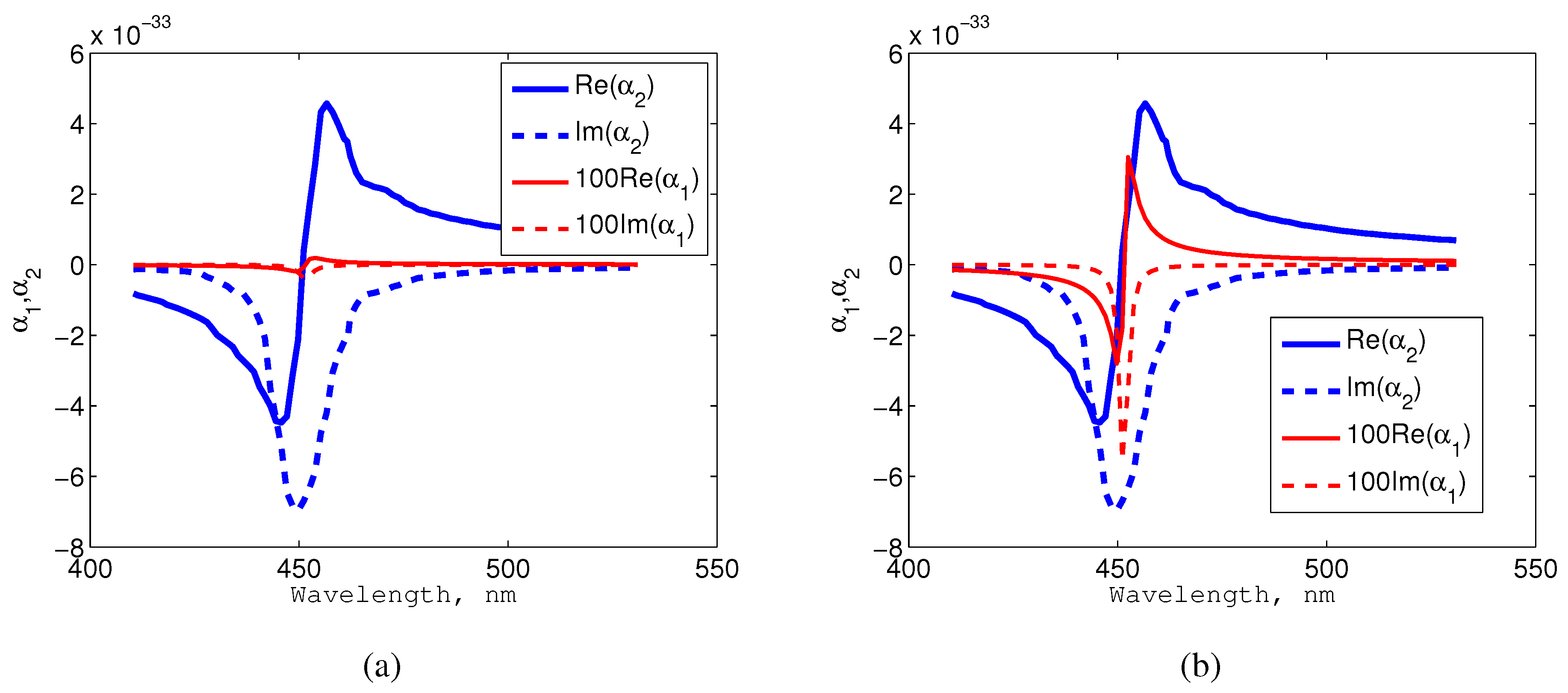
The results for $ECS/EC{S}_{\max }$ are presented in Figure 6. The qualitative agreement holds until $b=0.5$ nm, and this agreement is sufficient in order to claim that our approximate analytical model is quantitatively adequate. The spectral hole at 452–454 nm appears when $b=0.1$ nm, and this is clearly the Fano resonance and not the Rabi splitting, as is noticed in [16]. In the classification of the present paper, this case is referred to as SEFC/IMC. The corresponding plot of polarizabilities is shown in Figure 7a. The Fano modification of the spectrum occurs when the resonant polarizability of the QE is smaller than that of the NA by four orders of magnitude.

Figure 7. Complex polarizabilities of Elements 1 and 2 illuminated separately: (a) $d/e=0.1$ nm; (b) $d/e=0.7$ nm.

Figure 7. Complex polarizabilities of Elements 1 and 2 illuminated separately: (a) $d/e=0.1$ nm; (b) $d/e=0.7$ nm.

When $B\equiv d/e=0.3$ nm, the spectrum of ECS in Figure 6 combines the features of the Fano resonance and Rabi oscillations. The cases $B=0.5$ and $B=0.7$ nm clearly correspond to the Rabi splitting. However, all values of B in the range 0.1–0.7 nm still correspond to the case we called SEFC/IMC. Polarizabilities ${\alpha }_1$ and ${\alpha }_2$ for the case $B=0.7$ nm are depicted in Figure 7b. The resonant value of $|{\alpha }_1|$ is here lower than that of $|{\alpha }_2|$ by two orders of magnitude. This polarizability of the QE is still insufficient to implement the regime of SMC. The relative Rabi splitting is in this case equal 3.5%. This splitting is not yet accompanied by the damping of radiation, which is still enhanced.

Really, for the case $B=0.7$ nm, we obtained the values $|F_d|=37.42$ and $|F_d|=34.10$, respectively, at hybridized resonance wavelengths $\lambda =441$ and 462 nm. At both of these wavelengths, the value $|{\alpha }_1|$ is nearly equal to 2% of the resonant value $|{\alpha }_1\left({\omega }_0\right)|$. Therefore, $|{\alpha }_{\mathrm{tot}}|$ at $\lambda =441$ and 462 nm is only slightly smaller than the value $|{\alpha }_1|$ at the individual resonance of the QE. Respectively, the overall extinction of the nanosystem is not suppressed compared to the single QE in spite of the noticeable Rabi splitting. The same refers to the overall fluorescence. This is still the regime SEFC IMC in our classification.

Higher values of d (for which there are no data in [16]) in our calculations may correspond to stronger Rabi splitting and to a more noticeable decrease of the overall fluorescence compared to that of the single QE. The value $B=0.9$ nm corresponds to the relative Rabi splitting 5% and to the decrease of $|{\alpha }_{\mathrm{tot}}\left({\omega }_{\pm }\right)|$ by one order of magnitude compared to $|{\alpha }_1\left({\omega }_0\right)|$. The same damping level obviously refers to the fluorescence. This regime would correspond to SMC, i.e., non-radiative Rabi oscillations or fluorescence quenching.

3.2. Discussion

Above, we have presented an express-analysis of our formulas based on the equivalent circuits of two coupled antennas, which quantitatively describe the quantum emitter and the plasmonic nanoparticle forming the plasmon-enhanced fluorescence system. This express-analysis is validated via the comparison of the present model with the literature data. We think that our analysis is helpful for studying the plasmon-enhanced fluorescence by newcomers and may be also useful for experienced researchers working in the field.

Its main educational merit is the simple deterministic model of Rabi oscillations and fluorescence quenching. Both of these effects (especially the second one) are still considered by the majority of researchers as quantum effects. In our deep conviction, the nature of these effects is as classical as that of the Purcell effect. Even the fluorescence quenching effects is simply a classical non-radiative coupling of two dipole antennas, which may happen even for collinear dipoles due to hybridization of their resonances. In this regime, QE and NA mutually suppress their radiation resistances. Of course, the semiclassical model and even the purely quantum model also correctly describe these effects. However, they hardly bring anything qualitatively new. The role of the quantum theory is two-fold: it is capable of properly describing the nonlinear effects, which we ignore, and of properly determining the bounds of validity for the classical model (mainly concerning the pumping level).

In the modern literature, our point of view can be met. Classical interpretation of Rabi oscillations is quite popular, and corresponding works have been already mentioned above. The quenching in plasmon-enhanced fluorescence is seldom treated as a classical effect. One of these rare works is [10], where this effect was claimed to be classical. If we accept this point of view, the following question arises: does the fluorescence quench for sufficiently strong mutual coupling of two dipoles or does this obviously implies high-order multipoles? In [29] (where the fluorescence quenching is also claimed to be a classical effect), the quenching arises due to the coupling of a quantum dot to high-order multipole modes excited in the NA. These modes, in accordance with [29], receive all of the near-field power from the QE and dissipate it, because higher multipoles radiate weakly. If the dipole mode is induced in the NA, this, in accordance with [29], results in the high Purcell factor, and the fluorescence quenches only if high-order modes dominate.

We disagree with this claim. In our model, the quenching nicely occurs within the framework of the dipole model. In this model, it occurs not for all QEs. However, all QEs possessing the SEFC must experience the quenching when they approach too closely to the NA, and the mutual coupling becomes strong. The quenching mainly results from the strong detuning, which obviously accompanies the strong hybridization of the resonance. At frequencies ${\omega }_{\pm }$ located too far from ${\omega }_0$, the resonance magnitude of the dipole moments of both NA and QE is small compared to the case of the individual resonances. Moreover, their dipole moments at these frequencies turn out to be out-of phase, and the total dipole moment is smaller than their arithmetic sum. This regime is called in the antenna theory either the non-radiative coupling regime or the dark mode regime and is known for two dipole antennas.

As for the multipole modes of NAs, they may be noticeable for NAs more complex than the single metal nanosphere or dimer of nanospheres. However, we believe that for any mode, it is possible to build its equivalent circuit and to reveal the same effects that we have analyzed for the dipole modes of Objects 1 and 2. The enhancement due to the Purcell effect and the quenching due to the hybridization may hold for the near-field interaction of any multipole moments. For the simple-shape structures, like in Figure 1, these fine effects may provide correction terms to the factors obtained within the framework of the dipole model.

To conclude this discussion, let us notice that our model is applicable even to so-called spacers [30]. The spacer is a generator of localized surface plasmon excited by the fluorescence of a QE (or several QEs). The feedback is offered by the strong near-field mutual coupling of the QE and the Ag or Au nanoparticle. Our system in the case of SMC becomes the spacer on the condition of the very high pumping. Then, the nonlinear instability is developed, and the system passes the generation threshold, i.e., the coherent plasmon arises in the NA. Though this coupling is non-radiative, the dipole moment of the system in the over-threshold regime is not fully suppressed, and the spacer emits a small amount of coherent light. The coherency of this light can be seen from the dramatic squeezing of the Lorentzian line of radiation centered at the plasmon resonance. The linewidth becomes by one order of magnitude narrower than that described by the Lorentzian damping factor ${\gamma }_2$ Equation (25). Before the regime, when the plasmon and its radiation become coherent, the transition process occurs. This process is non-linear, and this non-linearity restricts the oscillation amplitude.

At first glance, our linear model, which implies modest pumping of the QE, has nothing to do with this regime. However, in [17], it was shown that the transition regime in any spacer starts from non-radiative (fluorescence quenching holds!) Rabi oscillations. In accordance with the semiclassical theory of [17], these oscillations occur in the background of the modulation instability and represent an initial process of the over-threshold dynamics of the spacer. After some dozens of Rabi periods, the non-linear auto-oscillations competing with this linear process [31] replace non-radiative Rabi oscillations, and the transition regime continues towards the steady regime. If there were no fluorescence quenching, the power absorbed from pumping would be radiated, and auto-oscillations could not develop.

Finally, let us try to guess why the model of the fluorescence quenching presented in this paper has not been published before. This seems strange, because the explanation in terms of the suppressed dipole moment $d_{\mathrm{tot}}$ is simplest. The dipoles of QE and NA, which are strongly mutually coupled, suppress one another; their mutual resistances compensate the radiation resistances, and the mode of their oscillation is dark. Probably, it was not understood earlier because the dipole moments of the QE and NA are collinear. In both optical and radio communities, there is conviction that the coupling of collinear dipoles is constructive for radiation (whereas the coupling of two parallel dipoles is destructive). Really, a high Purcell is known for the case when the dipoles of our system are collinear. High Raman gain is known for a molecule emitting the Raman radiation enhanced by a collinear dipole of the plasmonic nanoparticle. Parallel components of the dipole moment interact destructively; both Purcell and Raman gains for parallel dipoles are smaller than unity. In the theory of wire antennas [25], it is stated that, unlike two parallel dipoles, a collinear passive wire enhances the radiation of the active one. However, in the antenna theory, resonant collinear wire dipoles are never strongly coupled. Their centers are always distanced from one another at least by the total length of two arms. As for the molecule in the scheme of surface-enhanced Raman scattering, it is also never strongly coupled to the plasmonic particles, because it is not resonant. Its Raman radiation is emitted at different frequencies. Therefore, the destructive mutual coupling of two collinear resonant dipoles making their total dipole moment close to zero has not been sufficiently studied. The radio analogue of the non-radiative Rabi oscillations can be imaged as a coaxial system of active and passive wire antennas both performed as helices with resonant total length and a very small height to allow the strong mutual coupling. Such systems can be definitely used for wireless power transfer.

4. Conclusions

In this paper, we have suggested a classical circuit model of the hybridized oscillations in the system of a quantum emitter coupled to a nanoantenna. We concentrate on the case when the pumping is sufficiently weak and results only in the spontaneous emission called fluorescence. The role of the NA in this fluorescence can be either constructive (Purcell effect) or destructive (fluorescence quenching). Furthermore, the NA may strongly modify the fluorescence spectrum compared to the Lorentzian line of the single QE. This modification may have the shape of either the Fano resonance or the Rabi oscillations.

All of these phenomena are described by a newly-introduced circuit model. Our model generalizes the earlier classical model suggested to describe some properties of spontaneous emission in the presence of classical resonators [18]. It also corrects the previously-suggested circuit model [21]. Our model is based on the near-field interaction, which takes into account the inductive, capacitive and resistive components of the coupling. Two last components turn out to be mutually balanced. Therefore, the dispersion equation turns out to be equivalent to that of two resonant inductively-coupled circuits. However, the dipole model of the coupling allows a much more deep and extended analysis of the fluorescence spectra than a purely qualitative study allowed by the inductive model. In this way, we obtained the correct result for the Rabi frequency and good agreement with the numerical results of the semiclassical model for fluorescence and extinction spectra. An even more important merit of this model is the quantitative description of the fluorescence quenching. This happens even for collinear dipoles of both QE and NA. When their resonant mutual coupling is strong, the total dipole moment is suppressed, though its spectrum retains the shape of Rabi oscillations.

The predicting capacity of the model implies that it does not describe a classical analogue of the realistic nanosystem, such as a couple of pendulums. It really describes the realistic processes in the realistic nanosystem, because all effects under study—the Purcell effect, self-induced Rabi oscillations and fluorescence quenching—are, in fact, classical phenomena. From our insight, they all represent some features of the electromagnetic coupling of an active transmitting antenna to a passive antenna element.

Our model is purely dipole and does not involve higher multipoles (earlier involved in order to explain the fluorescence quenching in a classical way). Therefore, it is very simple. Interestingly, the simple linear model turns out to be applicable even to the surface-plasmon nanolaser, the so-called spacer, where it describes the initial stage of the transition regime over the generation threshold.

References

- Bauch, M.; Toma, K.; Toma, M.; Zhang, Q.; Dostalek, J. Plasmon-Enhanced Fluorescence Biosensors: A Review. Plasmonics 2014, 9, 781–799. [Google Scholar] [CrossRef]
- Purcell, E.M. Spontaneous emission probabilities at radio frequencies. Phys. Rev. 1946, 69, 681. [Google Scholar]
- Agio, M.; Martin-Cano, D. Nano-optics: The Purcell factor of nanoresonators. Nat. Phot. 2013, 7, 674–675. [Google Scholar] [CrossRef]
- Novotny, L.; Hecht, B. Principles of Nano-Optics; Cambridge University Press: Cambridge, UK, 2006; pp. 453–456. [Google Scholar]
- Bharadwaj, P.; Novotny, L. Spectral dependence of single molecule fluorescence enhancement. Opt. Express 2007, 15, 14266–14274. [Google Scholar] [CrossRef] [PubMed]
- Acuna, G.P.; Moller, F.M.; Holzmeister, P.; Beater, S.; Lalkens, B.; Tinnefeld, P. Fluorescence Enhancement at Docking Sites of DNA-Directed Self-Assembled Nanoantennas. Science 2012, 338, 506–510. [Google Scholar] [CrossRef] [PubMed]
- Sauvan, C.; Hugonin, J.P.; Maksymov, I.S.; Lalanne, P. Theory of the spontaneous optical emission of nanosize photonic and plasmon resonators. Phys. Rev. Lett. 2013, 110, 237401. [Google Scholar] [PubMed]
- Gabrielse, G.; Dehmelt, H. Observation of Inhibited Spontaneous Emission. Phys. Rev. Lett. 1985, 55, 67–70. [Google Scholar] [PubMed]
- Dulkeith, E.; Ringler, M.; Klar, T.A.; Feldmann, J. Gold Nanoparticles Quench Fluorescence by Phase Induced Radiative Rate Suppression. Nano Lett. 2005, 5, 585–588. [Google Scholar] [CrossRef] [PubMed]
- Anger, P.; Bharadwaj, P.; Novotny, L. Enhancement and Quenching of Single-Molecule Fluorescence. Phys. Rev. Lett. 2006, 96, 113002. [Google Scholar] [CrossRef] [PubMed]
- Gérard, J.-M. Solid-State Cavity Quantum Electrodynamics with Self-Assembled Quantum Dots. Top. Appl. Phys. 2003, 90, 269–314. [Google Scholar]
- Akimov, A.V.; Mukherjee, A.; Yu, C.L.; Chang, D.E.; Zibrov, A.S.; Hemmer, P.R.; Park, H.; Lukin, M.D. Generation of single optical plasmons in metallic nanowires coupled to quantum dots. Nature 2007, 450, 402–406. [Google Scholar] [CrossRef] [PubMed]
- Kaluzny, Y.; Goy, P.; Gross, M.; Raimond, J.M.; Haroche, S. Observation of Self-Induced Rabi Oscillations in Two-Level Atoms Excited Inside a Resonant Cavity: The Ringing Regime of Superradiance. Phys. Rev. Lett. 1983, 51, 1175–1178. [Google Scholar] [CrossRef]
- Zhu, Y.; Gauthier, D.J.; Morin, S.E.; Wu, Q.; Carmichael, H.J.; Mossberg, T.W. Vacuum Rabi Splitting as a Feature of Linear-Dispersion Theory: Analysis and Experimental Observations. Phys. Rev. Lett. 1990, 64, 2499–2502. [Google Scholar] [CrossRef] [PubMed]
- Raimond, J.-M.; Vitrant, G.; Haroche, S. Spectral line broadening due to interaction between very excited atoms: The dense Rydberg gas. J. Phys. B At. Mol. Phys. 1981, 14, L655. [Google Scholar] [CrossRef]
- Savasta, S.; Saija, R.; Ridolfo, A.; Di-Stefano, O.; Denti, P.; Borghese, F. Nanopolaritons: Vacuum Rabi Splitting with a Single Quantum Dot in the Center of a Dimer Nanoantenna. ACS Nano 2010, 4, 6369–6376. [Google Scholar] [CrossRef] [PubMed]
- Andrianov, E.S.; Pukhov, A.A.; Dorofeenko, A.V.; Vinogradov, A.P.; Lisyansky, A.A. Rabi oscillations in spacers during nonradiative plasmon excitation. Phys. Rev. B 2012, 85, 035405. [Google Scholar] [CrossRef]
- Rudin, S.; Reinecke, T.L. Oscillator model for vacuum Rabi splitting in microcavities. Phys. Rev. B 1999, 59, 10227–10233. [Google Scholar] [CrossRef]
- Bosco de Magalhaes, A.R.; d’Avila Fonseca, C.H.; Nemes, M.C. Classical and quantum coupled oscillators: Symplectic structure. Physica Scripta 2006, 74, 472–480. [Google Scholar] [CrossRef]
- Novotny, L. Strong coupling, energy splitting, and level crossings: A classical perspective. Amer. J. Phys. 2010, 78, 1199–1202. [Google Scholar] [CrossRef]
- Greffet, J.-J.; Laroche, M.; Marquier, F. Impedance of a Nanoantenna and a Single Quantum Emitter. Phys. Rev. Lett. 2010, 105, 117701. [Google Scholar] [CrossRef] [PubMed]
- Zengin, G.; Johansson, G.; Johansson, P.; Antosiewicz, T.J.; Käll, M.; Shegai, T. Approaching the strong coupling limit in single plasmonic nanorods interacting with J-aggregates. Sci. Rep. 2013, 3, 3074. [Google Scholar] [CrossRef] [PubMed]
- Krasnok, A.E.; Slobozhanyuk, A.P.; Simovski, C.R.; Tretyakov, S.A.; Poddubny, A.N.; Miroshnichenko, A.E.; Kivshar, Y.S.; Belov, P.A. Antenna model of the Purcell effect. 2015. [Google Scholar]
- Chen, X.-W.; Sandoghdar, V.; Agio, M. Coherent Interaction of Light with a Metallic Structure Coupled to a Single Quantum Emitter: From Superabsorption to Cloaking. Phys. Rev. Lett. 2013, 110, 153605. [Google Scholar] [CrossRef] [PubMed]
- Balanis, C. Antenna Theory: Analysis and Design, 3rd ed.; Wiley: New York, NY, USA, 2005. [Google Scholar]
- Matthaei, G.L.; Young, L.; Jones, E.M.T. Microwave Filters, Impedance-Matching Networks, and Coupling Structures; Artech House: Dordrecht, The Netherlands, 1980. [Google Scholar]
- Bohren, C.F.; Huffman, D.R. Absorption and Scattering of Light by Small Particles; Wiley: New York, NY, USA, 1983. [Google Scholar]
- Klimov, V.V. Nanoplasmonics; Pan Stanford Publishing: Singapore, 2011; p. 103. [Google Scholar]
- Sun, G.; Khurgin, J.B. Origin of giant difference between fluorescence, resonance, and nonresonance Raman scattering enhancement by surface plasmons. Phys. Rev. A 2012, 85, 063410. [Google Scholar] [CrossRef]
- Bergman, D.J.; Stockman, M.I. Surface Plasmon Amplification by Stimulated Emission of Radiation: Quantum Generation of Coherent Surface Plasmons in Nanosystems. Phys. Rev. Lett. 2003, 90, 027402. [Google Scholar] [CrossRef] [PubMed]
- Stockman, M.I. The spacer as a nanoscale quantum generator and ultrafast amplifier. J. Opt. 2010, 12, 024004. [Google Scholar] [CrossRef]
- Rogobete, L.; Kaminski, F.; Agio, M.; Sandoghdar, V. Design of plasmonic nanoantennae for enhancing spontaneous emission. Opt. Lett. 2007, 32, 1623–1625. [Google Scholar] [CrossRef] [PubMed]
- Ordal, M.A.; Bell, R.J.; Alexander, R.W.; Long, L.L.; Querry, M.R. Optical properties of fourteen metals in the infrared and far infrared: Al, Co, Cu, Au, Fe, Pb, Mo, Ni, Pd, Pt, Ag, Ti, V, and W. Appl. Opt. 1985, 24, 4493–4499. [Google Scholar] [CrossRef] [PubMed]
- Pokutnyi, S. Optical absorption at one-particle states of charge carriers in semiconductor quantum dots. J. Nanos. Chem. 2013, 3, 39. [Google Scholar] [CrossRef]
- Johnson, P.B.; Christy, R.W. Optical constants of the noble metals. Phys. Rev. B 1972, 6, 43701–43708. [Google Scholar] [CrossRef]
© 2015 by the author; licensee MDPI, Basel, Switzerland. This article is an open access article distributed under the terms and conditions of the Creative Commons Attribution license (http://creativecommons.org/licenses/by/4.0/).
Share and Cite
MDPI and ACS Style
Simovski, C. Circuit Model of Plasmon-Enhanced Fluorescence. Photonics 2015, 2, 568-593. https://doi.org/10.3390/photonics2020568
AMA Style
Simovski C. Circuit Model of Plasmon-Enhanced Fluorescence. Photonics. 2015; 2(2):568-593. https://doi.org/10.3390/photonics2020568
Chicago/Turabian StyleSimovski, Constantin. 2015. "Circuit Model of Plasmon-Enhanced Fluorescence" Photonics 2, no. 2: 568-593. https://doi.org/10.3390/photonics2020568