1. Introduction
Magnetic fields play an important role for different astrophysical objects and have a large influence on various physical processes. For example, the magnetic fields of galaxies [
1] change the trajectories of cosmic rays. Charged particles without magnetic fields would pass through the galaxy disc during several decades of millions of years, and we could not detect them. However, the magnetic fields cause their motion along spirals, and they can remain in the galaxies during billions of years [
2]. Another important appearance of the magnetic field is connected with the dark spots on the Sun, which are connected with the greatest intensity of the magnetic field in the convective zone [
3]. If we are speaking about the accretion discs surrounding neutron stars, black holes and white dwarfs, the magnetic field can describe the transition of the angular momentum between different parts of the disc [
4]. So, we can conclude, that the magnetic fields are important for different branches of astrophysics and corresponding phenomena.
From the observational point of view, the magnetic field can be studied using three basic mechanisms [
5]. The first one is connected with the so-called Zeeman effect. It describes the splitting of the spectral lines, which is based on the influence of the magnetic field on the atoms in the cosmic medium. However, this method can be used only for quite large magnetic fields on the Sun and maybe other stars. The second method is connected with the synchrotron emission [
6]. If the particles are situated in the medium with magnetic field, typical frequencies of the emission will change. This approach has been used for the first observational studies of the galactic magnetic field. The third method is based on the Faraday rotation of the polarization plane of the radio waves [
7]. If the wave passes through the magnetized medium, the rotation angle is proportional to the value of the magnetic field, squared wavelength and the electron density. Currently, it is the basic method of studying the magnetic fields in the galaxies [
8] and other celestial objects. It is necessary to say that for our galaxy, the pulsars are often used, and if we are speaking about other galaxies, we should take extragalactic sources. First, observational data [
1] were devoted to classical objects that are quite similar with the Milky Way, such as M31, M33 and M51. Currently, we have quite accurate observational results for several tens of galaxies. One of the most important results have been obtained by the CHANG-ES project, which give the calculations of the magnetic field based on the Faraday rotation data for 13 galaxies [
9].
The magnetic fields are usually described by the dynamo theory [
10,
11]. It is based on the transition of the kinetic energy of the conducting medium to the energy of the magnetic field. It is necessary to share both the small-scale dynamo, which is connected with the structure of the turbulent motions, and the large-scale one. The large-scale dynamo describes the evolution of the regular field, which is a result of averaging the fields by the typical length scales of turbulent cells. The evolution of the field is connected with joint action of the differential rotation (it is connected with nonsolid rotation of the object) and the alpha-effect that characterizes the vorticity of the turbulent motions. The magnetic field evolution is described by the Steenbeck—Krause—Raedler equation, which is obtained by averaging the magnetohydrodynamics equations [
12,
13].
However, obtaining the direct numerical solution of the Steenbeck—Krause—Raedler equation is quite difficult. The first problem is connected with the computational resources, which are large for the real objects because of large Reynolds and Prandtl numbers, so usually, such problems are solved only for some part of the object [
14]. The second problem is based on a large number of parameters characterizing the system. It is so high that we can obtain different results while changing them (it is necessary to mention that they are not known well). So, it is quite convenient to introduce two-dimensional models which take into account different symmetries of the objects and can be analyzed in a simple way.
As for the objects with the shape of a disc, usually, the so-called no-
z approximation is taken [
13,
15]. It takes into account the fact that the magnetic field is quite close to the equatorial plane, so the vertical component of the field can be neglected in some cases, and its
z-derivatives can be obtained by the solenoidality conditions. Such model can be effectively used to model the magnetic field in galaxies and in the accretion discs.
The dynamo mechanism described the exponential growth of the magnetic field [
16]. However, the magnetic field growth cannot be infinite in time, and it is restricted by the energy conservation law. If the magnetic field energy becomes comparable with the kinetic energy of the turbulent motions, the field growth should stop. This could be resolved by introducing the nonlinearity in the equations governing the process of the field growth [
11,
17]. So, the exponential growth will saturate after reaching some characteristic value of the magnetic field (it can be connected with the so-called equipartition value).
Numerical modeling shows different regimes of the saturation. The first one describes the monotonous growth, which stops if the field becomes close to the equipartition value. Another case is connected with the oscillations near the equipartition field. From the mathematical point of view, it is connected with the parameters of the system of differential equations. The nonlinear equations have different stable solutions. They can be associated with the nodes and focuses. In the first case, we shall have the monotonous saturation and in the second—the oscillatory regime [
18,
19].
The stable solutions of the equations can be analyzed using the first order of the perturbation theory, which is well-known in the theory of differential equations. We should solve the eigenvalue problem for this system, and the results of the eigenvalues will allow us to classify the types of the stability.
The paper is organized as following. At first, we describe the main features of the magnetic field evolution and present the equation of the no-z approximation. Then, we introduce the nonlinearity, which describes the saturation of the exponential growth of the solution. We also describe the stability of the solutions in the most general way. After that, we show the stability of the solution for concrete cases connected with the accretion discs. In the end, we present the results of numerical modeling, and it can be seen that the type of the saturation corresponds to the previous analytical models. We also discuss the magnetic fields in other astrophysical objects, such as the galaxies which have quite similar shape of the disc.
2. Basic Equations of the No-z Approximation
The large-scale magnetic field evolution is described by the Steenbeck—Krause—Raedler equation [
12]:
where
is the large-scale magnetic field,
is the alpha-effect coefficient,
is the large-scale velocity, and
is the turbulent diffusion coefficient.
If we are speaking about the objects that have the shape of the disc, we can take the cylindrical polar coordinates, and the disc will be described by the values:
We can assume that the field is mainly situated in the disc plane. We can also describe the axisymmetiric field. So, the main parts of the field are connected with the radial component and the azimuthal one [
20]:
As for the alpha-effect coefficient, we can take the model (it can be obtained, for example, using self-similar model [
21]):
where
is the characteristic value of the alpha-effect. It is connected with the Coriolis force in the rotating disc, which influences the turbulent velocity, and it can be described by the following simple estimates [
16]:
where
is the length scale of the turbulence.
The alpha-effect coefficient can be constructed using the formulae
[
10], but for the case of the disc, it is proportional to the angular velocity of the object [
16].
For the large-scale velocity, we can take the formula which is connected with the angular velocity
The equations of the field components can be written as [
18]:
where
is the radial part of the Laplace operator.
The magnetic field cannot grow if it becomes larger than the equipartition value, which is described by the formula [
19]:
where
is the typical turbulent velocity and
is the typical density of the medium. If the magnetic field if close to the equipartition value, the growth should stop. There are different mechanisms of the alpha-effect quenching (for example, we can consider the helicity fluxes [
22]), but for the simplest case, we can take the simple square term in the alpha-effect [
23]. It can be taken into account using the following equations:
We can measure the magnetic fields in units of
the distances in units of the outer radius of the object
R and the times in units of
So, the equations will be the following:
Here, characterizes alpha-effect, describes the differential rotation and shows the dissipation in the disc plane.
3. Stable Solutions of the Equations
The stable solution for the magnetic field can be obtained by assuming zero the time derivatives of the magnetic field components. We can assume that
[
18] (it corresponds to zero diffusion in the radial direction, but we take into account the main part connected with the vertical direction):
First, we can take the zero solution. However, it is much more interesting to take the following pairs of the solutions (which are called stable points):
and
If we describe small perturbations of the field near these values, it is convenient to introduce the following functions:
The linearized equation for them will be the following [
15]:
The perturbations grow according to the exponential law:
where
is the eigenvalue of the matrix of the system of Equations:
The character of the stable points is connected with the sign of the real part of (25). If it is negative, the point will be stable. We should say that if the value is complex, we will have the focus, and for purely real eigenvalues, the node will take place. If we have the node, the field will grow monotonously. For the focus, we shall have oscillations of the components of the magnetic field near the stable point.
The analysis of Formula (25) in the most general way is quite difficult. So, it is better to take concrete examples of the equations characterizing the specific rotation laws. In the following part, we are going to describe the solution for the Kepler rotation law, which can be used for the accretion discs surrounding such massive astrophysical objects as black holes, neutron stars and white dwarfs.
4. Stability for the Kepler Rotation Curve
As a specific example, we consider the Keplerian rotation curve, for which [
4]:
where
M is the mass of the central object and
G is the gravitational constant. It does not seem to take place in galactic cases widely, but has a special mathematical interest, and it can be suitable for other objects, such as the accretion discs [
24].
Then, for such an angular velocity, we can use the no-
z approximation [
24], and the equations for stationary solutions will look like this:
After substitution into the equation, we obtain:
After transformation, we get such solutions of the equation:
Now, find the degree of growth:
We substitute such equations for perturbations of the stable solutions:
We open the brackets and neglect the terms of the second order of smallness and take Equations (26) and (27) into account:
To find the characteristic numbers, we construct a determinant and equate it to zero.
Let us introduce the notation:
Making up the characteristic equation and solving, we get such eigenvalues:
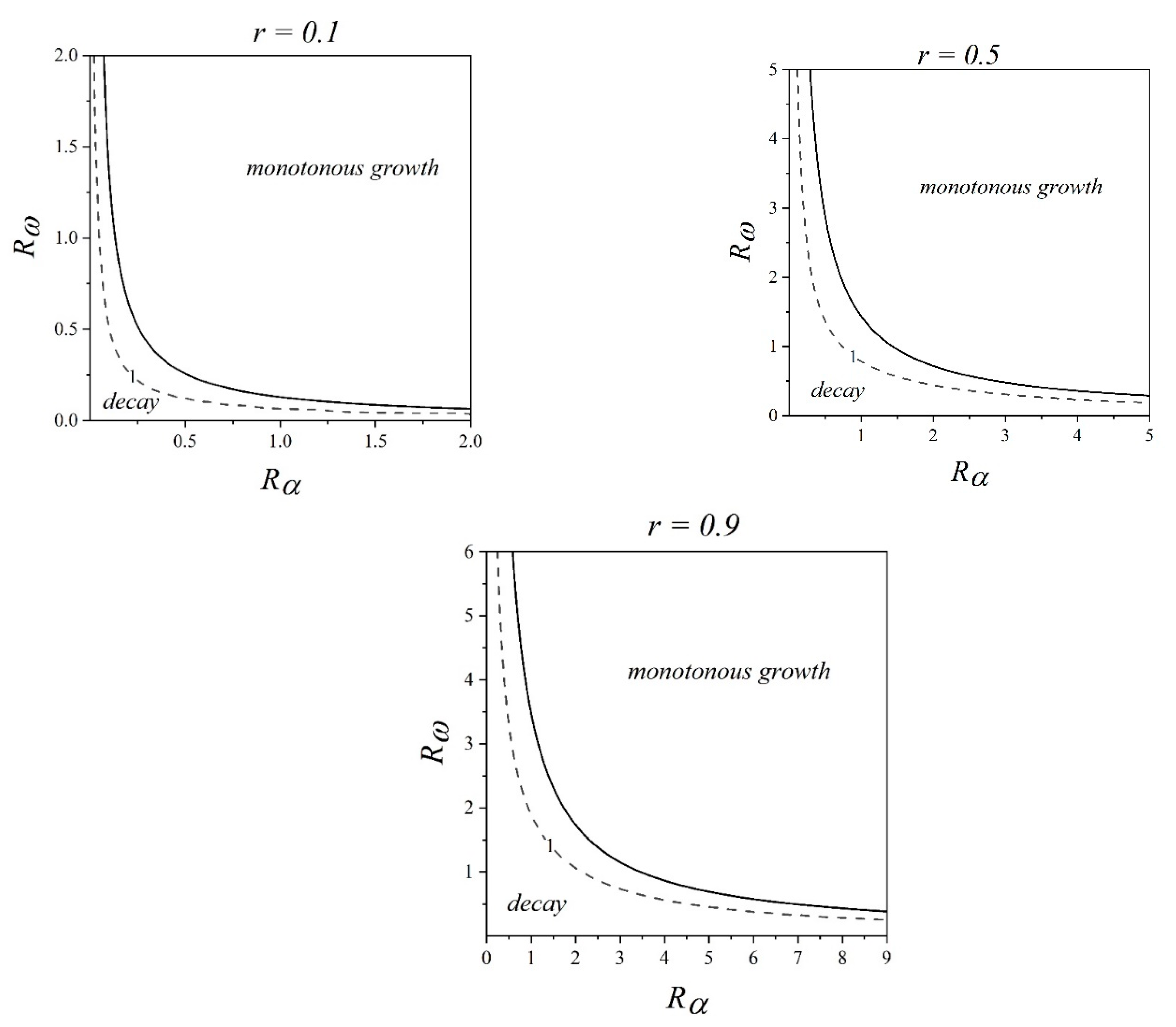
We can consider the radical expression:
The possibility that there will be a negative number under the root is described by the following condition:
In this case, the solution will reach a stationary value with fluctuations. Otherwise, there will be a monotonic output.
Thus, we got the function
; now, we can plot this function. We will be interested only in the area in which the value will be less than 1. Let us draw the corresponding level line. In addition, we draw a curve that will limit the growth region from the solution decay region. We get the following graphs (
Figure 1), where case
F < 1 is the decay region.
It is important to present concrete results, which can be useful to describe the regime of the magnetic field evolution in different cases. They are presented in
Table 1 (all values are measured in dimensionless units). Here, we showed typical values of the parameters which can characterize different astrophysical objects, such as galaxies and accretion discs. It is quite interesting to analyze the observational data about the accretion discs. Here, we take binary systems with a white dwarf as a primary star. Using the values of the outer radii of the discs and their masses, we can calculate their typical angular velocities. The half-thicknesses of the discs and turbulent velocities can be estimated taking model assumptions, so we can calculate the governing parameters [
24]. So, the result of analysis of observational data is included in
Table 1 as well. We give the value of the function F and the growth rate of the magnetic field which can be calculated as
, which can be used while estimating the magnetic field evolution in different cases.
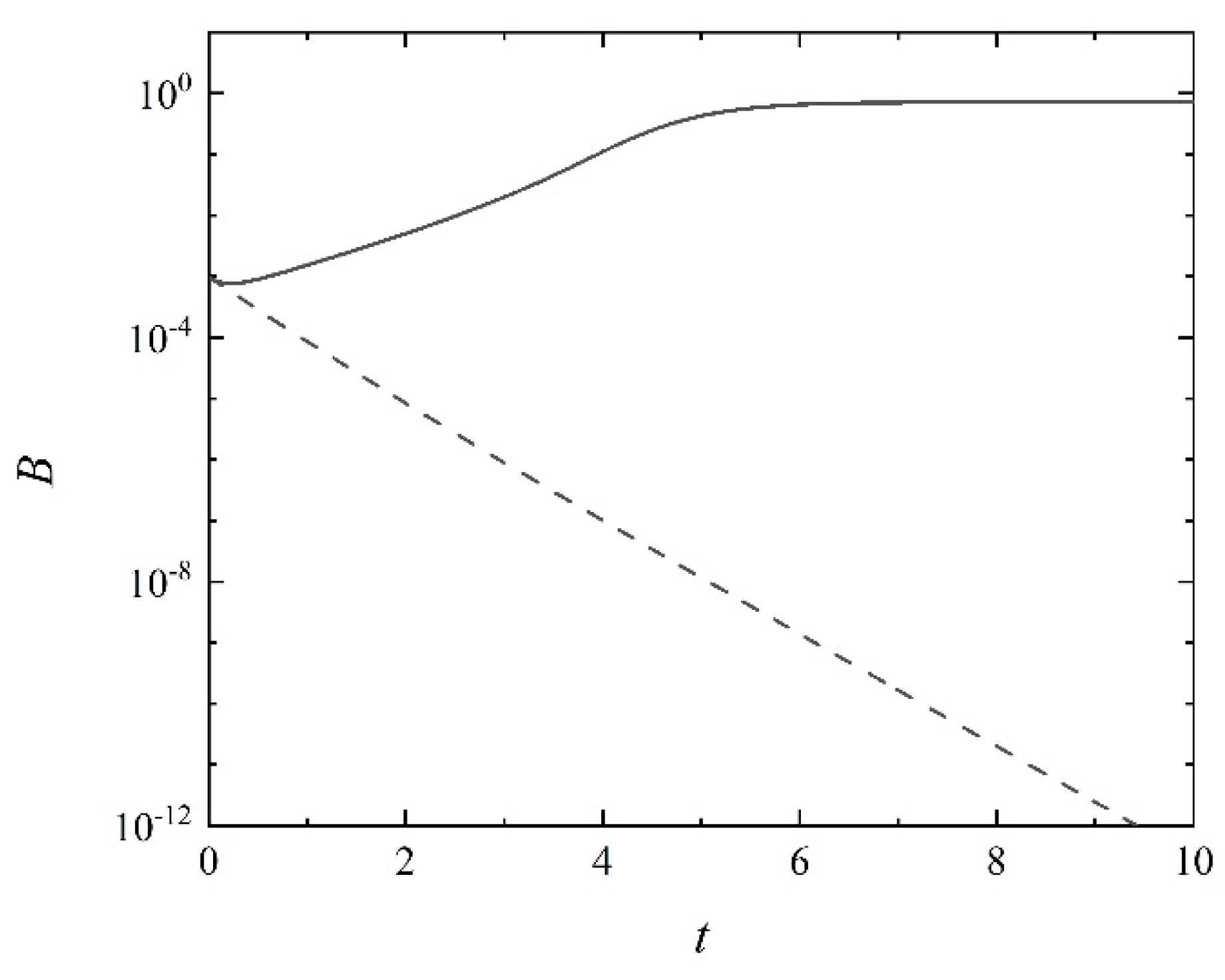
The magnetic field evolution for different
D is shown on
Figure 2. Here, the magnetic field is measured in equipartition values, and so it is dimensionless. The growth of the magnetic field (if it is possible) is exponential on the first stage; after that, it is stabilized. However, if we take other models [
21], we can obtain the power law.
Thus, we can see that the region of the oscillations of the magnetic field on the plot of the parameters fully corresponds to the decaying magnetic field. That means that the magnetic field can only grow monotonously, and for these values of the parameters, it is not possible to obtain the oscillating solutions.
5. Conclusions
We have studied the stability of the solutions of the system of dynamo equations in the no-z approximation, which describes the magnetic field generation in the discs. In the most general case, we have studied the stability of the solutions for different values of the parameters. Depending on the characteristics of the turbulence, we can have the focus (which is connected with monotonous growth) and the node (corresponding to oscillatory regime).
We have studied the concrete example of the model which corresponds to the Kepler rotation law. It was shown that for this case we can have only the monotonous solutions. Taking into account that such rotation law is connected with the accretion discs, it is necessary to say that for such objects, it is quite difficult to obtain the oscillatory regime, which is quite interesting from the observational point of view. However, for other objects, such as the galaxies, the numerical modeling shows [
15] that the magnetic field can have oscillations near the stable points. It would be quite interesting to test such results both for the accretion discs and the galaxies.
Of course, we have described a simple model of the magnetic field generation. It is possible to take other models of the magnetic fields. One of the most interesting approaches is connected with the self-similar approach, which has been described in [
21,
29,
30,
31]. It describes the magnetic field using the equations taking into account the turbulent diffusion and the alpha-effect, which are solved analytically. For the simplest case, the steady magnetic field can be described by exact solutions containing the hyperbolic sine, which corresponds to the “X-type” field structure. A wide range of solutions can be found using the Lagrange functions and hypergeometric ones. The time dependence of the magnetic field is also studied. The solution is self-similar in time, and it can be described by the exponential or power law. Such an approach can be interesting, and it is useful to study the magnetic field in the main parts of the galaxies and in the halo as well. However, our model takes slightly different model assumptions (which are connected with a specific Keplerian rotation law), so the field components are described by Formulae (32) and (33). In general, the result in the equatorial plane is the same with the “X-type” magnetic field, but there are some remarkable differences.


