
Iterative Tomographic Image Reconstruction Algorithm Based on Extended Power Divergence by Dynamic Parameter Tuning

 , , and
Abstract
1. Introduction
2. Proposed Method
2.1. Definition and Properties of EPD
2.2. Iterative Reconstruction Algorithm by Dynamic Parameter Tuning
| Algorithm 1 Procedure of PXEM algorithm |
Require: , , , , ,
|
| Algorithm 2 Procedure of PDEM algorithm |
Require: , , , , ,
|
2.3. Practical Strategy for Dynamic Parameter Tuning Using Reduced-Size System
| Algorithm 3 Procedure of PREM algorithm |
Require: , , , , , , , ,
|
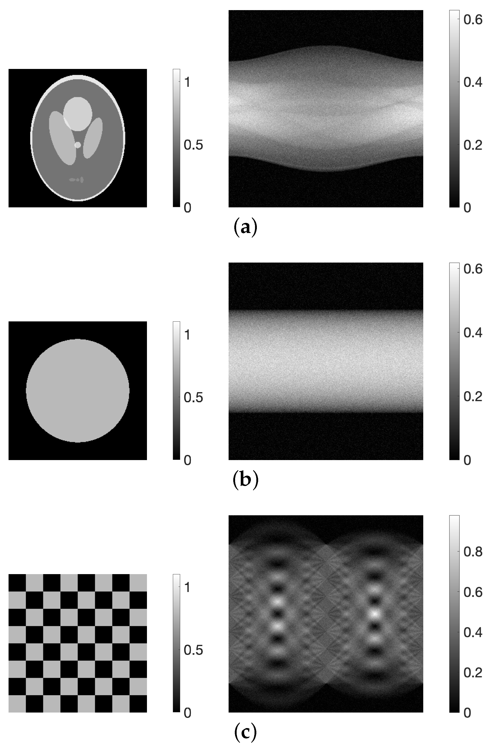
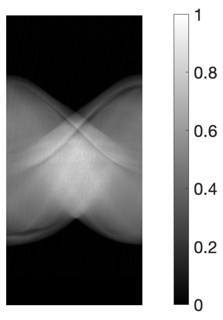
3. Experiment
3.1. Experimental Method
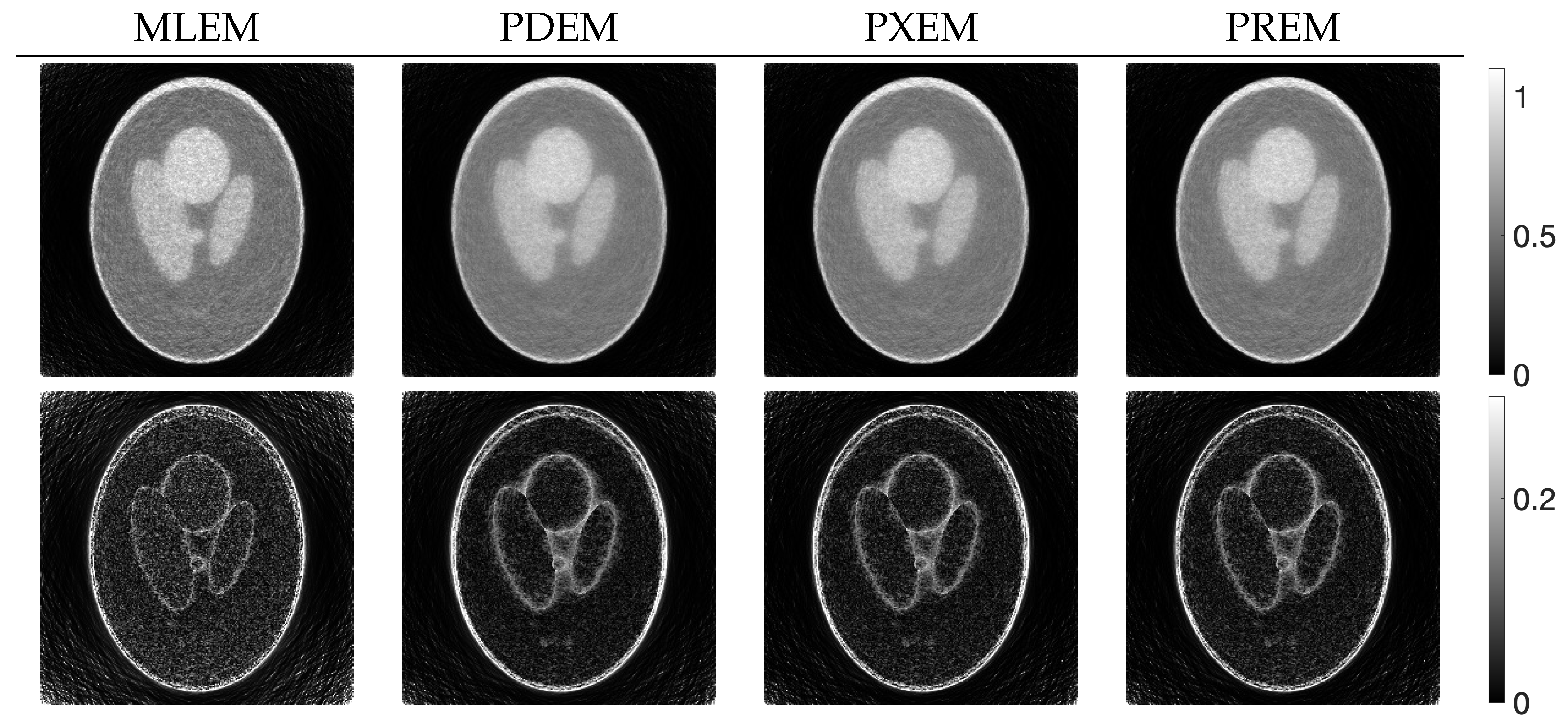
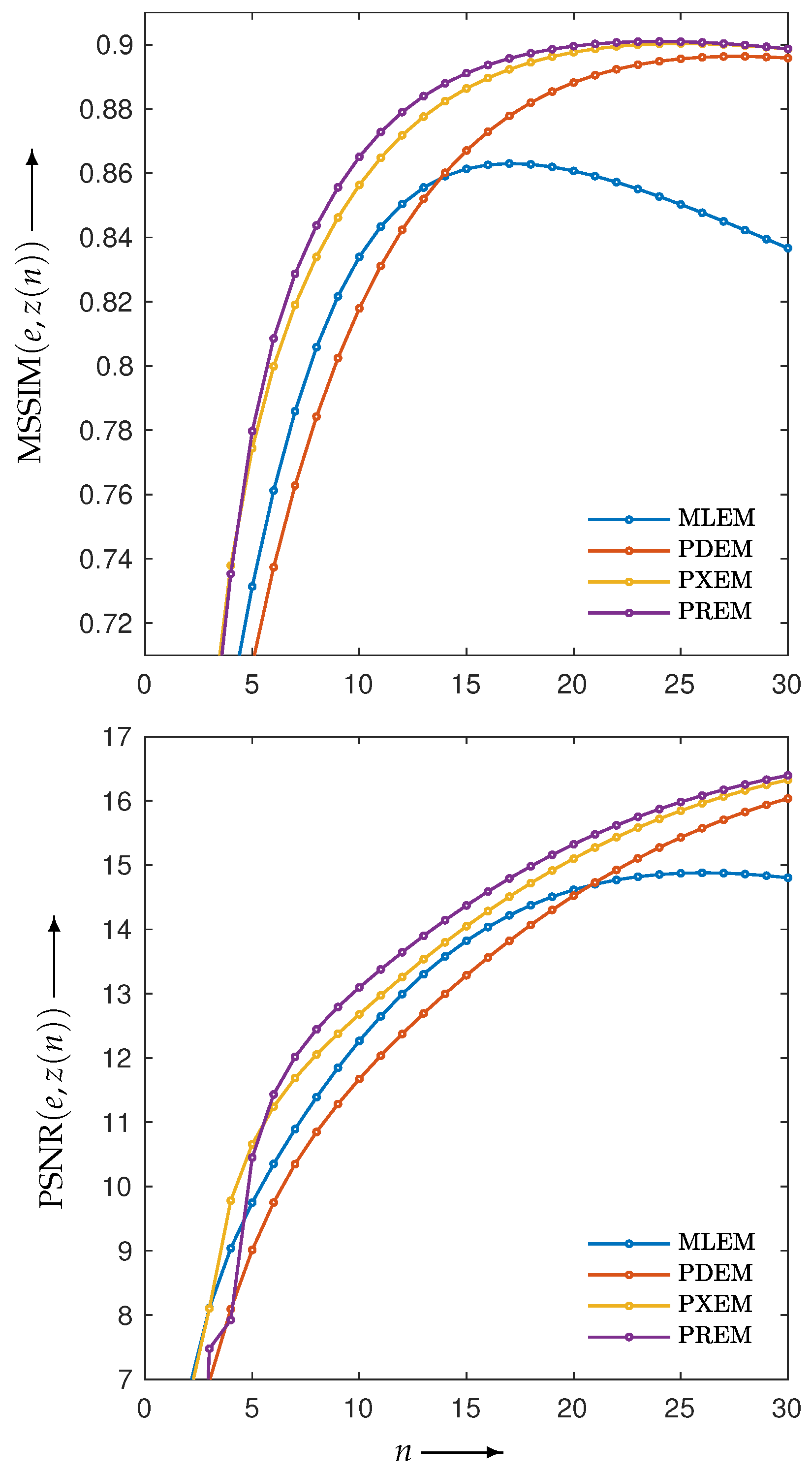
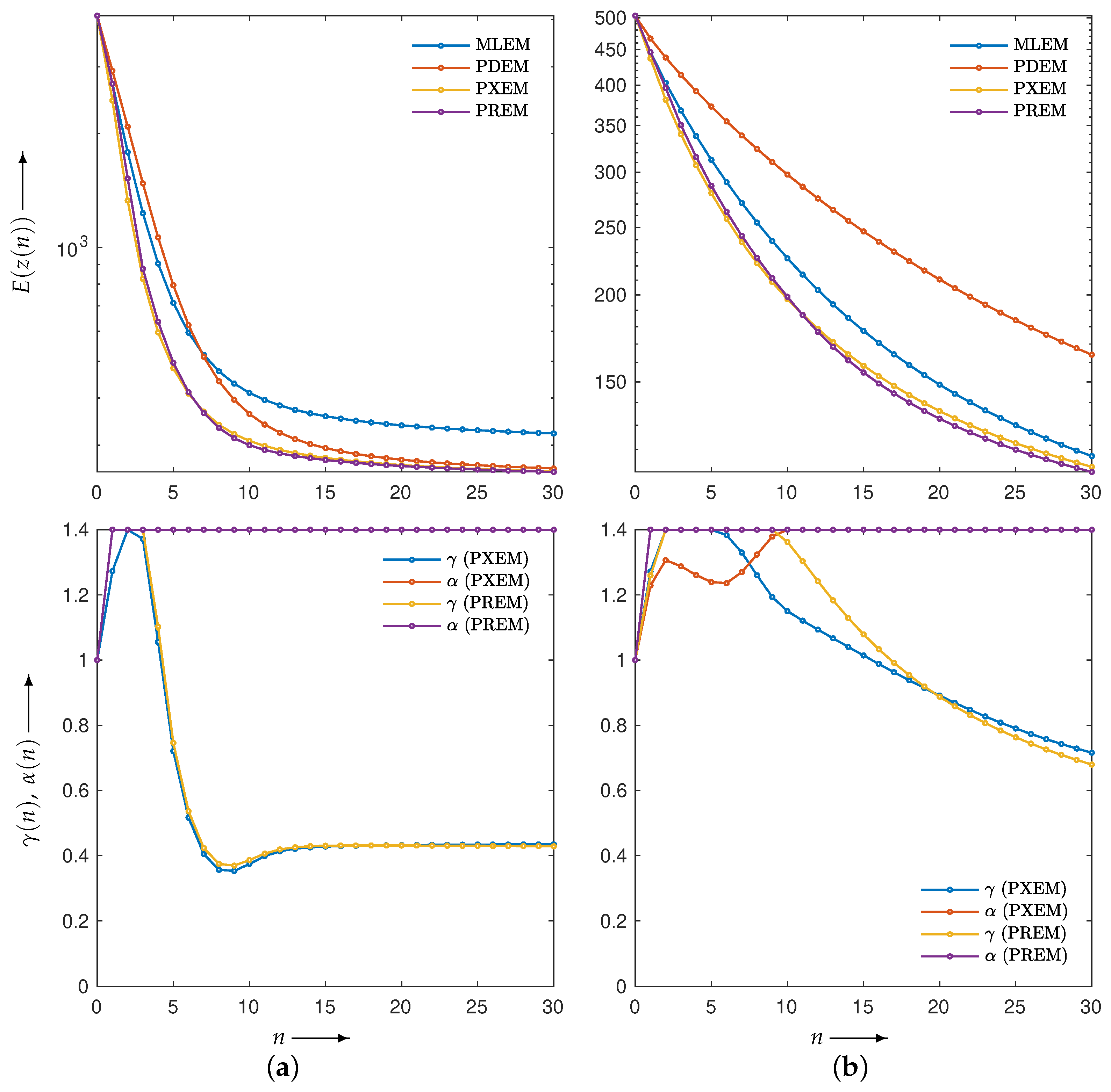
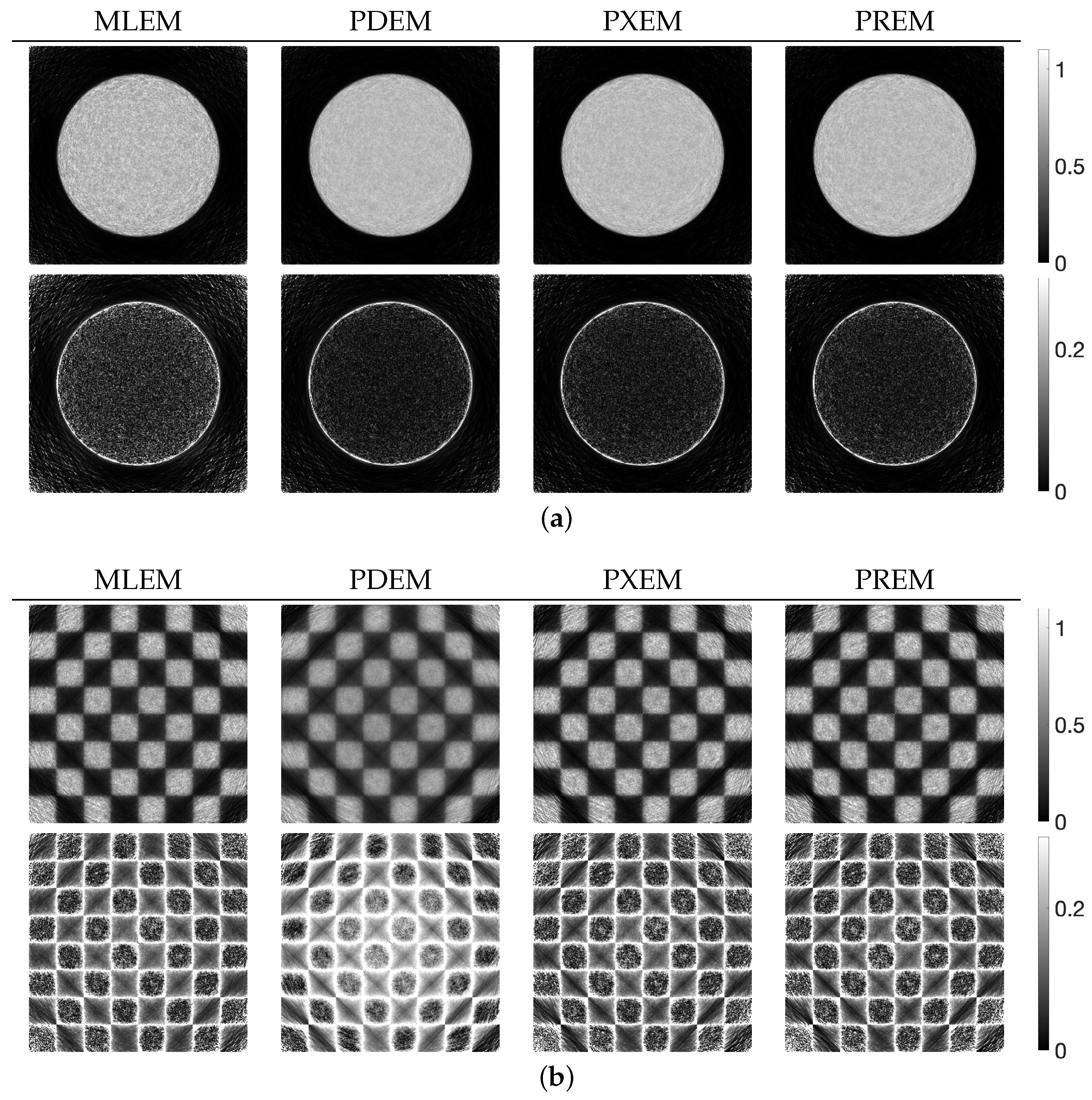
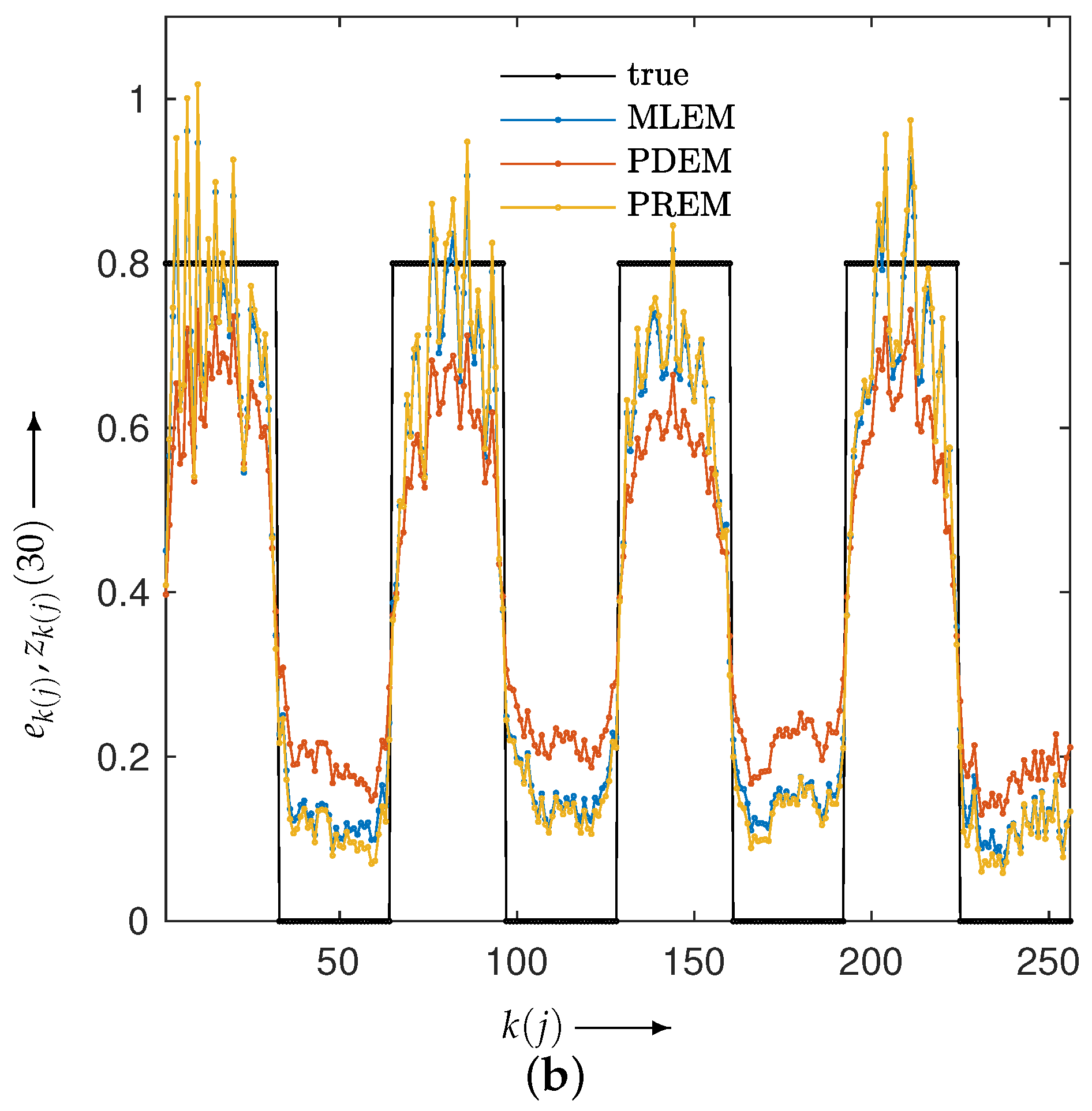
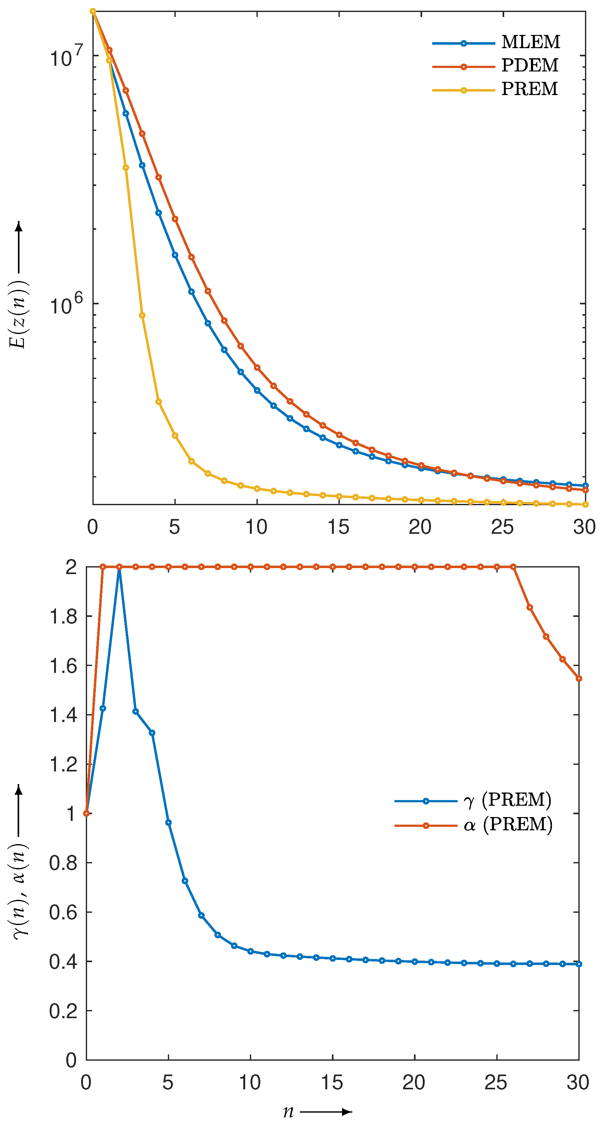
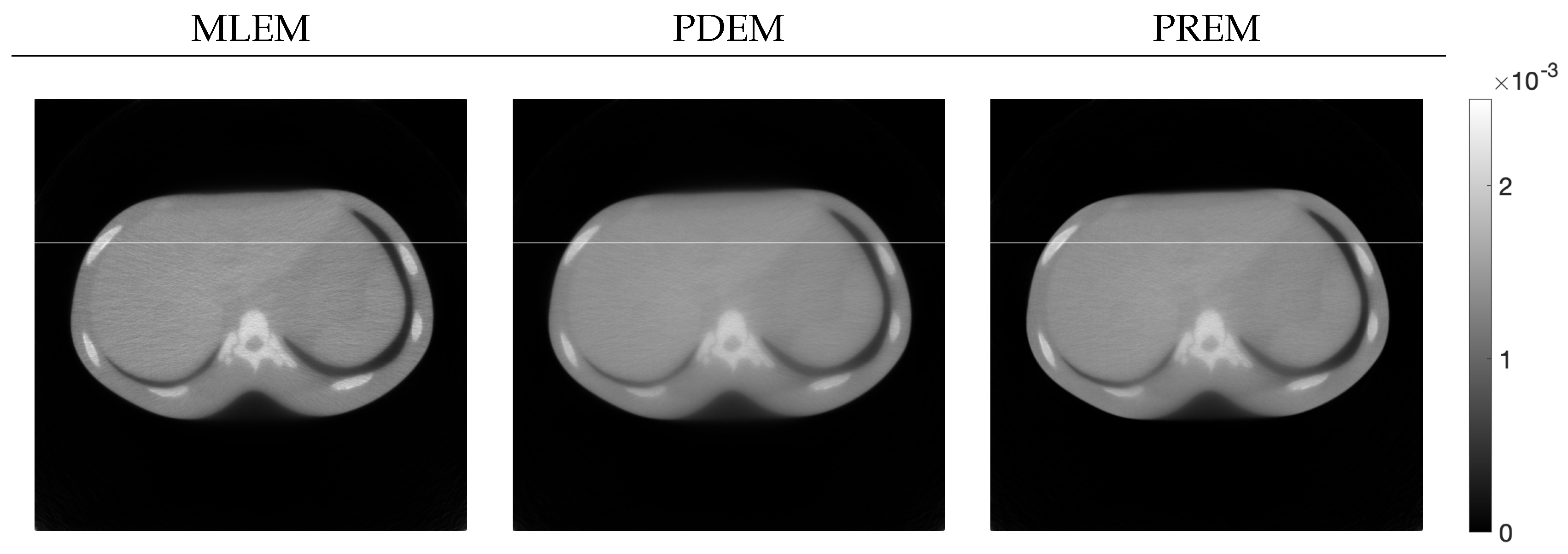
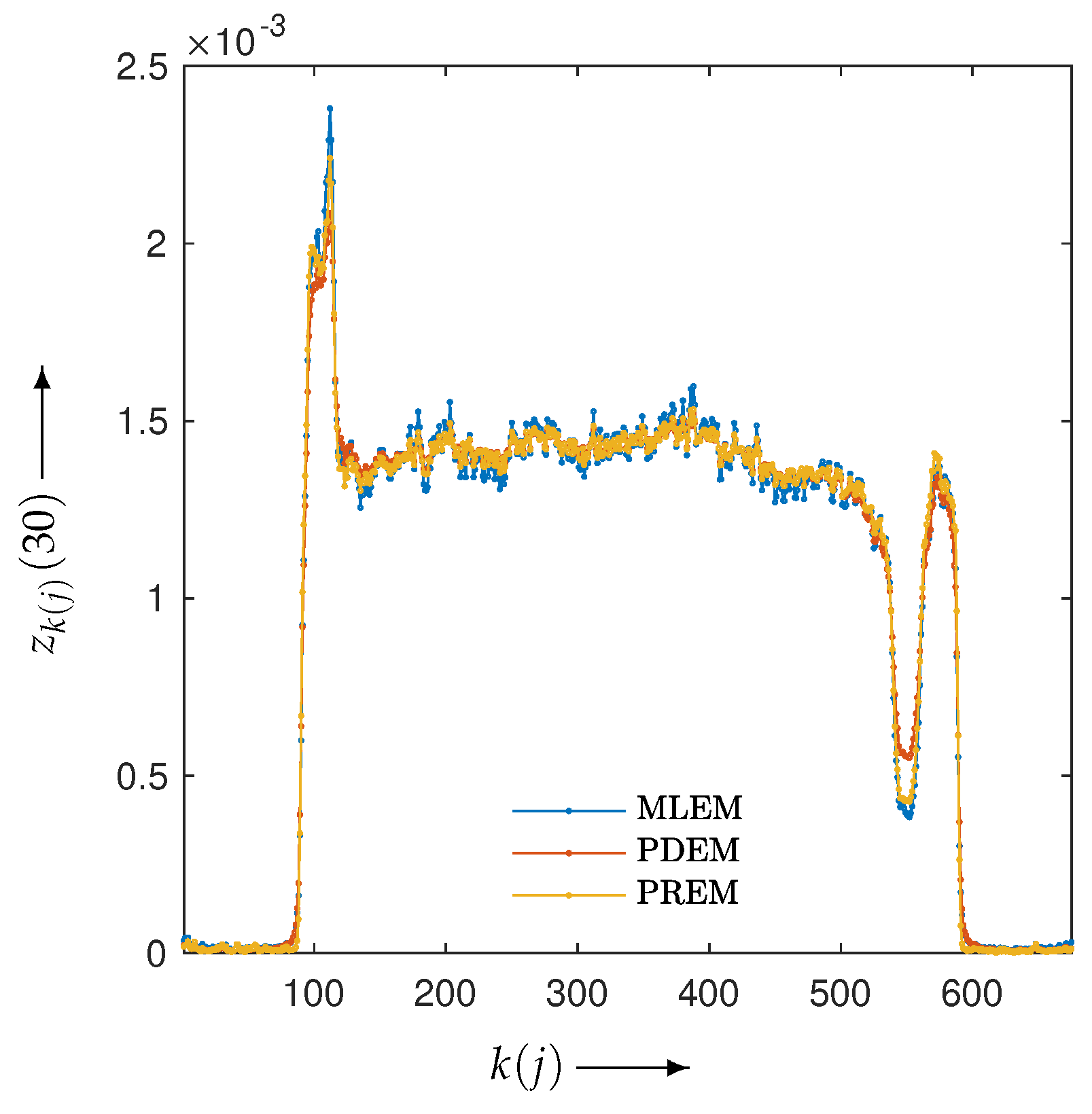
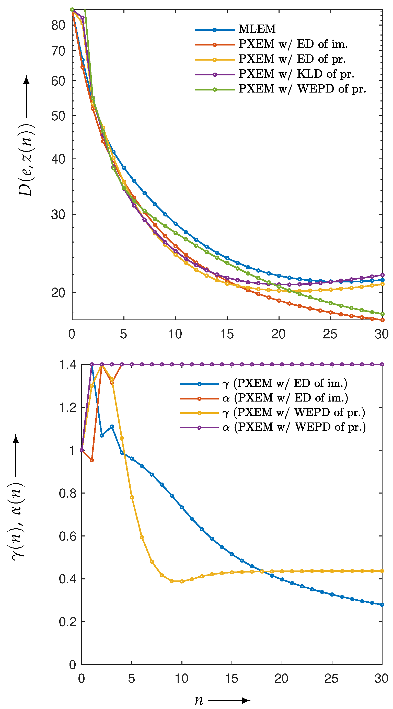
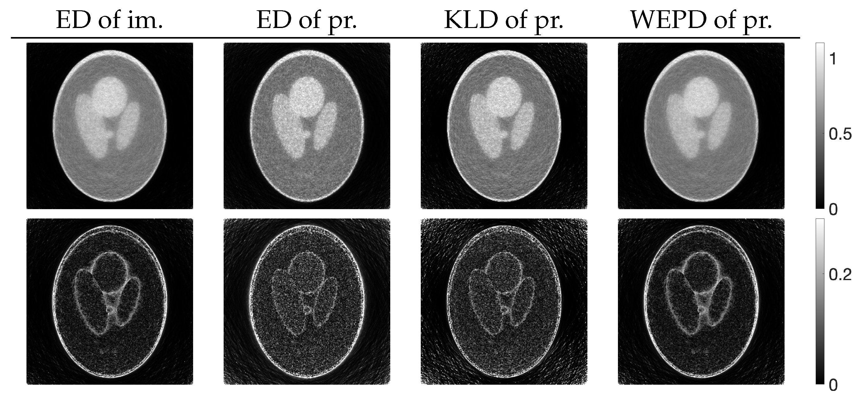
3.2. Experimental Results and Discussion
4. Conclusions
Author Contributions
Funding
Institutional Review Board Statement
Informed Consent Statement
Data Availability Statement
Conflicts of Interest
References
- Kak, A.C.; Slaney, M. Principles of Computerized Tomographic Imaging; IEEE Press: Piscataway, NJ, USA, 1988. [Google Scholar]
- Stark, H. Image Recovery: Theory and Application; Academic Press: Orlando, FL, USA, 1987. [Google Scholar] [CrossRef]
- Herman, G. Image Reconstruction from Projections. Fundamentals of Computerized Tomography; Advances in Computer Vision and Pattern Recognition; Springer: London, UK, 1980. [Google Scholar] [CrossRef]
- Seeram, E. Computed Tomography: Physical Principles, Clinical Applications, and Quality Control, 4th ed.; Elsevier: Amsterdam, The Netherlands, 2015. [Google Scholar]
- Gordon, R.; Bender, R.; Herman, G. Algebraic Reconstruction Techniques (ART) for three-dimensional electron microscopy and X-ray photography. J. Theor. Biol. 1970, 29, 471–481. [Google Scholar] [CrossRef] [PubMed]
- Badea, C.; Gordon, R. Experiments with the nonlinear and chaotic behaviour of the multiplicative algebraic reconstruction technique (MART) algorithm for computed tomography. Phys. Med. Biol. 2004, 49, 1455–1474. [Google Scholar] [CrossRef] [PubMed]
- Seibert, J.A. Iterative reconstruction: How it works, how to apply it. Pediatr. Radiol. 2014, 44, 431–439. [Google Scholar] [CrossRef] [PubMed]
- Geyer, L.L.; Schoepf, U.J.; Meinel, F.G.; Nance, J.W.; Bastarrika, G.; Leipsic, J.A.; Paul, N.S.; Rengo, M.; Laghi, A.; De Cecco, C.N. State of the Art: Iterative CT Reconstruction Techniques. Radiology 2015, 276, 339–357. [Google Scholar] [CrossRef] [PubMed]
- Qiu, D.; Seeram, E. Does Iterative Reconstruction Improve Image Quality and Reduce Dose in Computed Tomography? Radiology 2016, 1, 42–54. [Google Scholar] [CrossRef]
- Shepp, L.; Vardi, Y. Maximum Likelihood Reconstruction for Emission Tomography. IEEE Trans. Med. Imaging 1982, 1, 113–122. [Google Scholar] [CrossRef] [PubMed]
- Byrne, C.L. Block-iterative methods for image reconstruction from projections. IEEE Trans. Image Process. 1996, 5, 792–794. [Google Scholar] [CrossRef]
- Darroch, J.N.; Ratcliff, D. Generalized Iterative Scaling for Log-Linear Models. Ann. Math. Stat. 1972, 43, 1470–1480. [Google Scholar] [CrossRef]
- Katsekpor, T. Convergence of the Multiplicative Algebraic Reconstruction Technique for the Inconsistent System of Equations. Oper. Res. Forum 2023, 4, 88. [Google Scholar] [CrossRef]
- Mohammadinejad, P.; Mileto, A.; Yu, L.; Leng, S.; Guimaraes, L.S.; Missert, A.D.; Jensen, C.T.; Gong, H.; McCollough, C.H.; Fletcher, J.G. CT Noise-Reduction Methods for Lower-Dose Scanning: Strengths and Weaknesses of Iterative Reconstruction Algorithms and New Techniques. RadioGraphics 2021, 41, 1493–1508. [Google Scholar] [CrossRef] [PubMed]
- Lee, J.; Baek, J. Iterative reconstruction for limited-angle CT using implicit neural representation. Phys. Med. Biol. 2024, 69, 105008. [Google Scholar] [CrossRef]
- Zhang, M.; Gu, S.; Shi, Y. The use of deep learning methods in low-dose computed tomography image reconstruction: A systematic review. Complex Intell. Syst. 2022, 8, 5545–5561. [Google Scholar] [CrossRef]
- Koetzier, L.R.; Mastrodicasa, D.; Szczykutowicz, T.P.; van der Werf, N.R.; Wang, A.S.; Sandfort, V.; van der Molen, A.J.; Fleischmann, D.; Willemink, M.J. Deep Learning Image Reconstruction for CT: Technical Principles and Clinical Prospects. Radiology 2023, 306, e221257. [Google Scholar] [CrossRef] [PubMed]
- Byrne, C.L. A unified treatment of some iterative algorithms in signal processing and image reconstruction. Inverse Probl. 2004, 20, 103–120. [Google Scholar] [CrossRef]
- Byrne, C.L. Block-Iterative Algorithms. Int. Trans. Oper. Res. 2009, 16, 427–463. [Google Scholar] [CrossRef]
- Beister, M.; Kolditz, D.; Kalender, W.A. Iterative reconstruction methods in X-ray CT. Phys. Medica 2012, 28, 94–108. [Google Scholar] [CrossRef] [PubMed]
- Kasai, R.; Yamaguchi, Y.; Kojima, T.; Yoshinaga, T. Tomographic Image Reconstruction Based on Minimization of Symmetrized Kullback-Leibler Divergence. Math. Probl. Eng. 2018, 9, 8973131. [Google Scholar] [CrossRef]
- Kasai, R.; Yamaguchi, Y.; Kojima, T.; Abou Al-Ola, O.M.; Yoshinaga, T. Noise-Robust Image Reconstruction Based on Minimizing Extended Class of Power-Divergence Measures. Entropy 2021, 23, 1005. [Google Scholar] [CrossRef] [PubMed]
- Kojima, T.; Yoshinaga, T. Iterative Image Reconstruction Algorithm with Parameter Estimation by Neural Network for Computed Tomography. Algorithms 2023, 16, 60. [Google Scholar] [CrossRef]
- Lu, W.; Yin, F. Adaptive algebraic reconstruction technique. Med. Phys. 2004, 31, 3222–3230. [Google Scholar] [CrossRef]
- Lin, C.; Zang, J.; Qing, A. Algebraic reconstruction technique with adaptive relaxation parameter based on hyperplane distance and data noise level. In Proceedings of the 2016 IEEE MTT-S International Conference on Numerical Electromagnetic and Multiphysics Modeling and Optimization (NEMO), Beijing, China, 27–29 July 2016. [Google Scholar] [CrossRef]
- Oliveira, N.; Mota, A.; Matela, N.; Janeiro, L.; Almeida, P. Dynamic relaxation in algebraic reconstruction technique (ART) for breast tomosynthesis imaging. Comput. Methods Programs Biomed. 2016, 132, 189–196. [Google Scholar] [CrossRef] [PubMed]
- Abou Al-Ola, O.M.; Fujimoto, K.; Yoshinaga, T. Common Lyapunov Function Based on Kullback–Leibler Divergence for a Switched Nonlinear System. Math. Probl. Eng. 2011, 2011, 723509. [Google Scholar] [CrossRef]
- Tateishi, K.; Yamaguchi, Y.; Abou Al-Ola, O.M.; Yoshinaga, T. Continuous Analog of Accelerated OS-EM Algorithm for Computed Tomography. Math. Probl. Eng. 2017, 2017, 1564123. [Google Scholar] [CrossRef]
- Wang, Z.; Simoncelli, E.P.; Bovik, A.C. Multiscale structural similarity for image quality assessment. In Proceedings of the The Thrity-Seventh Asilomar Conference on Signals, Systems & Computers, 2003, Pacific Grove, CA, USA, 9–12 November 2003; Volume 2, pp. 1398–1402. [Google Scholar] [CrossRef]
- Kullback, S.; Leibler, R.A. On Information and Sufficiency. Ann. Math. Stat. 1951, 22, 79–86. [Google Scholar] [CrossRef]
- Shepp, L.; Logan, B.F. The Fourier reconstruction of a head section. IEEE Trans. Nucl. Sci. 1974, 21, 21–43. [Google Scholar] [CrossRef]
- Kagaku, K. CT Whole Body Phantom PBU-60. Available online: https://www.kyotokagaku.com/en/products_data/ph-2b/ (accessed on 1 June 2024).
- Beran, R. Minimum Hellinger Distance Estimates for Parametric Models. Ann. Stat. 1977, 5, 445–463. [Google Scholar] [CrossRef]
- Beran, R. An Efficient and Robust Adaptive Estimator of Location. Ann. Stat. 1978, 6, 292–313. [Google Scholar] [CrossRef]
- Ishikawa, K.; Yamaguchi, Y.; Abou Al-Ola, O.M.; Kojima, T.; Yoshinaga, T. Block-Iterative Reconstruction from Dynamically Selected Sparse Projection Views Using Extended Power-Divergence Measure. Entropy 2022, 24, 740. [Google Scholar] [CrossRef]


| MLEM | PDEM | PXEM | PREM | |
|---|---|---|---|---|
| std. dev. | 0.083 | 0.056 | 0.056 | 0.057 |
| contrast | 0.532 | 0.418 | 0.544 | 0.550 |
Disclaimer/Publisher’s Note: The statements, opinions and data contained in all publications are solely those of the individual author(s) and contributor(s) and not of MDPI and/or the editor(s). MDPI and/or the editor(s) disclaim responsibility for any injury to people or property resulting from any ideas, methods, instructions or products referred to in the content. |
© 2024 by the authors. Licensee MDPI, Basel, Switzerland. This article is an open access article distributed under the terms and conditions of the Creative Commons Attribution (CC BY) license (https://creativecommons.org/licenses/by/4.0/).
Share and Cite
Yabuki, R.; Yamaguchi, Y.; Abou Al-Ola, O.M.; Kojima, T.; Yoshinaga, T. Iterative Tomographic Image Reconstruction Algorithm Based on Extended Power Divergence by Dynamic Parameter Tuning. J. Imaging 2024, 10, 178. https://doi.org/10.3390/jimaging10080178
Yabuki R, Yamaguchi Y, Abou Al-Ola OM, Kojima T, Yoshinaga T. Iterative Tomographic Image Reconstruction Algorithm Based on Extended Power Divergence by Dynamic Parameter Tuning. Journal of Imaging. 2024; 10(8):178. https://doi.org/10.3390/jimaging10080178
Chicago/Turabian StyleYabuki, Ryuto, Yusaku Yamaguchi, Omar M. Abou Al-Ola, Takeshi Kojima, and Tetsuya Yoshinaga. 2024. "Iterative Tomographic Image Reconstruction Algorithm Based on Extended Power Divergence by Dynamic Parameter Tuning" Journal of Imaging 10, no. 8: 178. https://doi.org/10.3390/jimaging10080178
APA StyleYabuki, R., Yamaguchi, Y., Abou Al-Ola, O. M., Kojima, T., & Yoshinaga, T. (2024). Iterative Tomographic Image Reconstruction Algorithm Based on Extended Power Divergence by Dynamic Parameter Tuning. Journal of Imaging, 10(8), 178. https://doi.org/10.3390/jimaging10080178