New Jacobi Galerkin Operational Matrices of Derivatives: A Highly Accurate Method for Solving Two-Point Fractional-Order Nonlinear Boundary Value Problems with Robin Boundary Conditions

Abstract

A novel numerical scheme is developed in this work to approximate solutions (APPSs) for nonlinear fractional differential equations (FDEs) governed by Robin boundary conditions (RBCs). The methodology is founded on a spectral collocation method (SCM) that uses a set of basis functions derived from generalized shifted Jacobi (GSJ) polynomials. These basis functions are uniquely formulated to satisfy the homogeneous form of RBCs (HRBCs). Key to this approach is the establishment of operational matrices (OMs) for ordinary derivatives (Ods) and fractional derivatives (Fds) of the constructed polynomials. The application of this framework effectively reduces the given FDE and its RBC to a system of nonlinear algebraic equations that are solvable by standard numerical routines. We provide theoretical assurances of the algorithm’s efficacy by establishing its convergence and conducting an error analysis. Finally, the efficacy of the proposed algorithm is demonstrated through three problems, with our APPSs compared against exact solutions (ExaSs) and existing results by other methods. The results confirm the high accuracy and efficiency of the scheme.

1. Introduction

Fractional differential equations (FDEs) have been the subject of heightened interest in recent decades owing to their robust capacity to represent memory and hereditary characteristics across various physical and engineering systems. These equations have been widely utilized in diverse domains, including economics [1], continuum and statistical mechanics [2], anomalous diffusion [3], viscoelasticity and vibration analysis [4], electrical circuit modeling [5], stability analysis [6], control theory [7], stochastic processes [8], time-delay systems [9], bio-engineering [10], and the fields of viscoelasticity and control theory [11,12]. In contrast to traditional differential equations (DEs), FDEs permit non-integer order derivatives, offering a more adaptable and precise mathematical framework for systems where the influence of past states affects present behavior; this capacity renders them vital in the analysis of complex dynamical systems.

Significant advancements have been made over time in extending and refining the models of FDEs to better model real-world complexities. A notable refinement is the increased use of the Liouville–Caputo fractional derivative (LCFD), which offers distinct advantages over the classical Riemann–Liouville Fds. Unlike the Riemann–Liouville Fds, the LCFD allows for the incorporation of more physically meaningful initial conditions, boundary conditions, and mixed conditions related to integer-order derivatives. This capability is particularly crucial in fields such as engineering, physics, and finance, where initial states are often described by measurable physical quantities. In this paper, we focus on the boundary value problem (BVP)

$$\stackrel{LC}{a}{\mathbb{D}}_{\xi }^{{\alpha }_2}\mathcal{Q}\left(\xi \right)=\mathcal{F}(\xi ,\mathcal{Q}\left(\xi \right),\stackrel{LC}{a}{\mathbb{D}}_{\xi }^{{\alpha }_1}\mathcal{Q}\left(\xi \right)),\xi \in (a,b),$$

(1)

subject to the RBCS

$${\beta }_1\mathcal{Q}\left(a\right)+{\beta }_2{\mathcal{Q}}^{\prime }\left(a\right)={\mathcal{C}}_1,{\gamma }_1\mathcal{Q}\left(b\right)+{\gamma }_2{\mathcal{Q}}^{\prime }\left(b\right)={\mathcal{C}}_2,$$

(2)

where $0<{\alpha }_1\le 1,1<{\alpha }_2<2,$ and $\stackrel{LC}{a}{\mathbb{D}}_{\xi }^{{\alpha }_1},\stackrel{LC}{a}{\mathbb{D}}_{\xi }^{{\alpha }_2}$ are LCFDs.

To the best of our knowledge, BVP (1)–(2) still lack numerical approaches for computing APPSs; this gap motivates us to develop a new numerical method that can effectively address this question and provide accurate solutions for complex scenarios.

The three main classifications of spectral methods are the collocation, tau, and Galerkin approaches. These methods are essential for obtaining numerical solutions (NUMSs) for a wide range of mathematical models: DEs [13], partial DEs [14,15,16,17,18], and FDEs [19,20,21].

They produce highly APPSs for various types of DEs while requiring relatively few unknowns. The choice of the most appropriate method depends on the characteristics of the DEs being examined and the specific boundary conditions involved. These approaches employ OMs to create efficient algorithms that provide accurate NUMSs for many forms of mathematical models: ordinary DEs [22,23,24], ordinary FDEs [25,26,27,28], partial FDEs [29], fractional integro-differential equation [30] thereby reducing the required computational effort.

To date, and to the best of our knowledge, no application of the Galerkin OM (GOM) to solve BVPs (1) and (2) using any basis function that meets the HRBCs has been reported in the literature. This gap partially drives our interest in employing such OMs for the numerical handling of this problem. The main objectives of this paper can be summarized as follows:

(i)

Constructing a new class of basis polynomials, named Robin-Modified General Shifted Jacobi (RMGSJ) polynomials, that satisfy the HRBCs.

(ii)

Establishing OMs for Ods and Fds of RMGSJ polynomials.

(iii)

Constructing a numerical algorithm for solving FDE (1) with HRBCs based on SCM and the introduced OMs of Ods and Fds.

The organization of the paper is as follows: Section 2 provides the definitions and properties of an LCFD. In Section 3, we discuss the necessary formulas related to GSJ polynomials and RMGSJ polynomials. Section 4 focuses on constructing RMGSJ polynomials that satisfy the HRBCs. Section 5 is dedicated to developing new OMs for both of the Ods and Fds of RMGSJ polynomials to address BVPs (1) and (2). The application of SCM to solve (1) and (2) is explored in Section 6. In Section 7, the convergence and error estimates of the suggested approach are examined. Section 8 presents three problems along with comparisons to various other methods found in the literature. Finally, Section 9 summarizes the key conclusions.

2. Basic Definition of LCFD

In this section, we present the essential concepts and the fundamental tools that are necessary for developing the proposed technique [31].

Definition 1.

The LCFD of order ν will be denoted by $\stackrel{LC}{a}{\mathbb{D}}_{\xi }^{\nu }$ and is defined as follows:

$$\stackrel{LC}{a}{\mathbb{D}}_{\xi }^{\nu }f\left(\xi \right)={\displaystyle \frac{1}{\Gamma (n-\nu )}}\underset{a}{\overset{\xi }{\int }}{(\xi -\tau )}^{n-\nu -1}{f}^{\left(n\right)}\left(\tau \right)d\tau ,\xi >a,n-1<\nu \le n.$$

(3)

The LCFD operator has the following properties:

$$\begin{array}{ccc}\hfill \stackrel{LC}{a}{\mathbb{D}}_{\xi }^{\nu }C& =& 0,\left(Cisconstant\right),\hfill \end{array}$$

(4)

$$\begin{array}{ccc}\hfill \stackrel{LC}{a}{\mathbb{D}}_{\xi }^{\nu }{(\xi -a)}^{\gamma }& =& d_{\gamma }{(\xi -a)}^{\gamma -\nu },d_{\gamma }={\displaystyle \frac{\Gamma (\gamma +1)}{\Gamma (\gamma +1-\nu )}},\hfill \end{array}$$

(5)

$$\begin{array}{ccc}\hfill \stackrel{LC}{a}{\mathbb{D}}_{\xi }^{\nu }({\delta }_1{h}_1\left(\xi \right)+{\delta }_2{h}_2\left(\xi \right))& =& {\delta }_1{D}^{\nu }{h}_1\left(\xi \right)+{\delta }_2{D}^{\nu }{h}_2\left(\xi \right),\hfill \end{array}$$

(6)

$$\begin{array}{ccc}\hfill \stackrel{LC}{a}{\mathbb{D}}_{\xi }^{\nu }f\left(\xi \right)& =& D^{n}f\left(\xi \right),\nu =n,n=1,2,\dots ,D={\displaystyle \frac{d}{d\xi }}.\hfill \end{array}$$

(7)

3. An Overview on JPs and GJPs

The orthogonal JPs, ${\mathcal{G}}_n^{({\vartheta }_1,{\vartheta }_2)}\left(x\right)$, satisfy [32]:

$${\int }_{-1}^1{w}^{{\vartheta }_1,{\vartheta }_2}\left(x\right){\mathcal{G}}_n^{({\vartheta }_1,{\vartheta }_2)}\left(x\right){\mathcal{G}}_m^{({\vartheta }_1,{\vartheta }_2)}\left(x\right)dx=\left\{\begin{array}{cc}0,\hfill & m\ne n,\hfill \\ h_n^{({\vartheta }_1,{\vartheta }_2)},\hfill & m=n,\hfill \end{array}\right.$$

where $w^{{\vartheta }_1,{\vartheta }_2}\left(x\right)={(1-x)}^{{\vartheta }_1}{(1+x)}^{{\vartheta }_2}$ and $h_n^{({\vartheta }_1,{\vartheta }_2)}={\displaystyle \frac{2^{\lambda }\Gamma (n+{\vartheta }_1+1)\Gamma (n+{\vartheta }_2+1)}{n!(2n+\lambda )\Gamma (n+\lambda )}},\lambda ={\vartheta }_1+{\vartheta }_2+1$.

The shifted JPs defined on $[0,\mathcal{L}]$, denoted as ${\mathcal{G}}_n^{({\vartheta }_1,{\vartheta }_2)}(\mathfrak{Z};0,\mathcal{L})={\mathcal{G}}_n^{({\vartheta }_1,{\vartheta }_2)}(2\mathfrak{Z}/\mathcal{L}-1)$, are in accordance with

$${\int }_0^{\mathcal{L}}{w}_{0,\mathcal{L}}^{{\vartheta }_1,{\vartheta }_2}\left(\mathfrak{Z}\right){\mathcal{G}}_n^{({\vartheta }_1,{\vartheta }_2)}(\mathfrak{Z};0,\mathcal{L}){\mathcal{G}}_m^{({\vartheta }_1,{\vartheta }_2)}(\mathfrak{Z};0,\mathcal{L})d\mathfrak{Z}=\left\{\begin{array}{cc}0,\hfill & m\ne n,\hfill \\ {\left({\displaystyle \frac{\mathcal{L}}{2}}\right)}^{\lambda }{h}_n^{({\vartheta }_1,{\vartheta }_2)},\hfill & m=n,\hfill \end{array}\right.$$

where $w_{0,\mathcal{L}}^{{\vartheta }_1,{\vartheta }_2}\left(\mathfrak{Z}\right)={(\mathcal{L}-\mathfrak{Z})}^{{\vartheta }_1}{\mathfrak{Z}}^{{\vartheta }_2}$. These polynomials can be represented in power form as follows ([33], Section 11.3.4):

$${\mathcal{G}}_i^{({\vartheta }_1,{\vartheta }_2)}(\mathfrak{Z};0,\mathcal{L})=\sum _{k=0}^i{c}_k^{\left(i\right)}{\mathfrak{Z}}^k,$$

(8)

where

$$c_k^{\left(i\right)}={\displaystyle \frac{{(-1)}^{i-k}\Gamma (i+{\vartheta }_2+1)\Gamma (i+k+\lambda )}{{\mathcal{L}}^{k}k!(i-k)!\Gamma (k+{\vartheta }_2+1)\Gamma (i+\lambda )}}.$$

(9)

The GSJ polynomials defined in $[a,b]$ are denoted as

$${\mathcal{G}}_n^{({\vartheta }_1,{\vartheta }_2)}(\xi ;a,b)={\mathcal{G}}_n^{({\vartheta }_1,{\vartheta }_2)}\left({\displaystyle \frac{2\xi }{b-a}}-{\displaystyle \frac{a+b}{b-a}}\right)={\mathcal{G}}_n^{({\vartheta }_1,{\vartheta }_2)}\left({\displaystyle \frac{\xi \mathcal{L}}{b-a}};0,\mathcal{L}\right),$$

(10)

and then they satisfy

$${\int }_a^b{w}_{a,b}^{{\vartheta }_1,{\vartheta }_2}\left(\xi \right){\mathcal{G}}_n^{({\vartheta }_1,{\vartheta }_2)}(\xi ;a,b){\mathcal{G}}_m^{({\vartheta }_1,{\vartheta }_2)}(\xi ;a,b)d\xi =\left\{\begin{array}{cc}0,\hfill & m\ne n,\hfill \\ {\left({\displaystyle \frac{b-a}{2}}\right)}^{\lambda }{h}_n^{({\vartheta }_1,{\vartheta }_2)},\hfill & m=n,\hfill \end{array}\right.$$

where $w_{a,b}^{{\vartheta }_1,{\vartheta }_2}\left(\xi \right)={(b-\xi )}^{{\vartheta }_1}{(\xi -a)}^{{\vartheta }_2}$. The two relations here denoted as (8) and (10) lead to

$${\mathcal{G}}_i^{({\vartheta }_1,{\vartheta }_2)}(\xi ;a,b)=\sum _{k=0}^i{b}_k^{\left(i\right)}{(\xi -a)}^k,$$

(11)

where

$$b_k^{\left(i\right)}={\displaystyle \frac{{(-1)}^{i-k}\Gamma (i+{\vartheta }_2+1)\Gamma (i+k+\lambda )}{{(b-a)}^{k}k!(i-k)!\Gamma (k+{\vartheta }_2+1)\Gamma (i+\lambda )}}.$$

(12)

Formula (11) allows us to see that the qth-derivatives of GSJ polynomials have special values, as follows:

$$D^q{\mathcal{G}}_n^{({\vartheta }_1,{\vartheta }_2)}(a;a,b)=q!b_q^{\left(n\right)},n\ge q,q=0,1,2,\dots$$

(13)

4. Robin-Modified General Shifted Jacobi Polynomials

In this section, a novel class of polynomials, denoted by ${\mathfrak{M}}_k^{({\vartheta }_1,{\vartheta }_2)}\left(\xi \right)$, will be developed. We call them “Robin-Modified Generalized Shifted Jacobi Polynomials”, and they are designed to satisfy the given form of HRBs

$${\beta }_1{\mathfrak{M}}_k^{({\vartheta }_1,{\vartheta }_2)}\left(a\right)+{\beta }_{2}D{\mathfrak{M}}_k^{({\vartheta }_1,{\vartheta }_2)}\left(a\right)=0,$$

(14)

$${\gamma }_1{\mathfrak{M}}_k^{({\vartheta }_1,{\vartheta }_2)}\left(b\right)+{\gamma }_{2}D{\mathfrak{M}}_k^{({\vartheta }_1,{\vartheta }_2)}\left(b\right)=0.$$

(15)

Thus, we propose RMGSJ polynomials in the form

$${\mathfrak{M}}_k^{({\vartheta }_1,{\vartheta }_2)}\left(\xi \right)=({\xi }^2+{\mathcal{A}}_k\xi +{\mathcal{B}}_k){\mathcal{G}}_k^{({\vartheta }_1,{\vartheta }_2)}(\xi ;a,b),k=0,1,2,\dots ,$$

(16)

where ${\mathcal{A}}_k$ and ${\mathcal{B}}_k$ are unique constants such that ${\mathfrak{M}}_k^{({\vartheta }_1,{\vartheta }_2)}\left(\xi \right)$ satisfy the two conditions (14) and (15). Substitution of ${\mathfrak{M}}_k^{({\vartheta }_1,{\vartheta }_2)}\left(\xi \right)$ into (14) and (15) yields the two linear equations in the two unknowns ${\mathcal{A}}_k$ and ${\mathcal{B}}_k$:

$${\beta }_1(a^2+{\mathcal{A}}_{k}a+{\mathcal{B}}_k){\mathcal{G}}_k^{({\vartheta }_1,{\vartheta }_2)}(a;a,b)+{\beta }_2\left((2a+{\mathcal{A}}_k){\mathcal{G}}_k^{({\vartheta }_1,{\vartheta }_2)}(a;a,b)+(a^2+{\mathcal{A}}_{k}a+{\mathcal{B}}_k)D{\mathcal{G}}_k^{({\vartheta }_1,{\vartheta }_2)}(a;a,b)\right)=0,$$

(17)

$${\gamma }_1(b^2+{\mathcal{A}}_{k}b+{\mathcal{B}}_k){\mathcal{G}}_k^{({\vartheta }_1,{\vartheta }_2)}(b;a,b)+{\gamma }_2\left((2b+{\mathcal{A}}_k){\mathcal{G}}_k^{({\vartheta }_1,{\vartheta }_2)}(b;a,b)+(b^2+{\mathcal{A}}_{k}b+{\mathcal{B}}_k)D{\mathcal{G}}_k^{({\vartheta }_1,{\vartheta }_2)}(b;a,b)\right)=0.$$

(18)

This system can be solved using the Mathematica code found in Appendix A, and the use of some simplification tools for algebraic expressions in Mathematica yields

$${\displaystyle {\mathcal{A}}_k=\frac{1}{{\mathcal{M}}_k}\sum _{i=0}^4{\mathcal{A}}_{i,k}{k}^i,{\mathcal{B}}_k=\frac{1}{{\mathcal{M}}_k}\sum _{i=0}^4{\mathcal{B}}_{i,k}{k}^i,{\mathcal{M}}_k=\sum _{i=0}^4{\mathcal{M}}_{i,k}{k}^i,}$$

(19)

where

$$\left.\begin{array}{cc}\hfill {\mathcal{A}}_{0,k}=& ({\vartheta }_1+1)({\vartheta }_2+1)(b-a)(2a{\beta }_2{\gamma }_1+{\beta }_1({\gamma }_1(a-b)(a+b)-2b{\gamma }_2)),\hfill \\ \hfill {\mathcal{A}}_{1,k}=& -\left(({\vartheta }_1+{\vartheta }_2+1)({\beta }_2({\gamma }_1({\vartheta }_1+1)(a-b)(a+b)-2{\gamma }_2(a{\vartheta }_2+a+b{\vartheta }_1+b))-{\beta }_1{\gamma }_2({\vartheta }_2+1)(a-b)(a+b))\right),\hfill \\ \hfill {\mathcal{A}}_{2,k}=& {\beta }_1{\gamma }_2({\vartheta }_2+1)(a-b)(a+b)+{\beta }_2({\gamma }_2({\vartheta }_2^2(a+b)+2{\vartheta }_2({\vartheta }_1(a+b)+2a+b)+{\vartheta }_1({\vartheta }_1(a+b)+2(a+2b))+3(a+b))\hfill \\ \hfill & -{\gamma }_1({\vartheta }_1+1)(a-b)(a+b)),\hfill \\ \hfill {\mathcal{A}}_{3,k}=& 2{\beta }_2{\gamma }_2({\vartheta }_1+{\vartheta }_2+1)(a+b),\hfill \\ \hfill {\mathcal{A}}_{4,k}=& {\beta }_2{\gamma }_2(a+b),\hfill \end{array}\right\}$$

(20)

$$\left.\begin{array}{cc}\hfill {\mathcal{B}}_{0,k}=& ({\vartheta }_1+1)({\vartheta }_2+1)(a-b)({\beta }_2(b{\gamma }_1(2a-b)+2{\gamma }_2(a-b))+a{\beta }_1(b{\gamma }_1(a-b)+{\gamma }_2(a-2b))),\hfill \\ \hfill {\mathcal{B}}_{1,k}=& ({\vartheta }_1+{\vartheta }_2+1)({\beta }_2({\gamma }_2(a^2+a{\vartheta }_1(a-2b)+b{\vartheta }_2(b-2a)-4ab+b^2)+ab{\gamma }_1({\vartheta }_1+1)(a-b))-ab{\beta }_1{\gamma }_2({\vartheta }_2+1)(a-b)),\hfill \\ \hfill {\mathcal{B}}_{2,k}=& {\beta }_2({\gamma }_2(a^2-ab{\vartheta }_2^2+a{\vartheta }_1(a-b{\vartheta }_1-4b)+b{\vartheta }_2(-2a{\vartheta }_1-4a+b)-5ab+b^2)+ab{\gamma }_1({\vartheta }_1+1)(a-b))\hfill \\ \hfill & -ab{\beta }_1{\gamma }_2({\vartheta }_2+1)(a-b),\hfill \\ \hfill {\mathcal{B}}_{3,k}=& -2ab{\beta }_2{\gamma }_2({\vartheta }_1+{\vartheta }_2+1),\hfill \\ \hfill {\mathcal{B}}_{4,k}=& -ab{\beta }_2{\gamma }_2,\hfill \end{array}\right\}$$

(21)

$$\left.\begin{array}{cc}\hfill {\mathcal{M}}_{0,k}=& ({\vartheta }_1+1)({\vartheta }_2+1)(a-b)({\beta }_1({\gamma }_1(a-b)-{\gamma }_2)+{\beta }_2{\gamma }_1),\hfill \\ \hfill {\mathcal{M}}_{1,k}=& -\left(({\vartheta }_1+{\vartheta }_2+1)({\beta }_1{\gamma }_2({\vartheta }_2+1)(a-b)+{\beta }_2({\gamma }_2({\vartheta }_1+{\vartheta }_2+2)-{\gamma }_1({\vartheta }_1+1)(a-b)))\right),\hfill \\ \hfill {\mathcal{M}}_{2,k}=& {\beta }_2({\gamma }_1({\vartheta }_1+1)(a-b)-\left({\gamma }_2({\vartheta }_1+{\vartheta }_2)({\vartheta }_1+{\vartheta }_2+3)\right)-3{\gamma }_2)-{\beta }_1{\gamma }_2({\vartheta }_2+1)(a-b),\hfill \\ \hfill {\mathcal{M}}_{3,k}=& -2{\beta }_2{\gamma }_2({\vartheta }_1+{\vartheta }_2+1),\hfill \\ \hfill {\mathcal{M}}_{4,k}=& -{\beta }_2{\gamma }_2.\hfill \end{array}\right\}$$

(22)

The special values $D^q{\mathfrak{M}}_k^{({\vartheta }_1,{\vartheta }_2)}\left(a\right),(1\le q\le k+2)$ are needed throughout the paper and have the form

$$D^q{\mathfrak{M}}_k^{({\vartheta }_1,{\vartheta }_2)}\left(a\right)=(a^2+{\mathcal{A}}_{k}a+{\mathcal{B}}_k)D^q{\mathcal{G}}_k^{({\vartheta }_1,{\vartheta }_2)}(a;a,b)+q(2a+{\mathcal{A}}_k)D^{q-1}{\mathcal{G}}_k^{({\vartheta }_1,{\vartheta }_2)}(a;a,b)+q(q-1)D^{q-2}{\mathcal{G}}_k^{({\vartheta }_1,{\vartheta }_2)}(a;a,b).$$

(23)

5. Operational Matrix of Derivatives of RMGSJ Polynomials

This section presents and proves two main theorems, which provide the two OMs for Ods and the LCFD related to the vector

$${\mathfrak{M}}_N^{({\vartheta }_1,{\vartheta }_2)}\left(\xi \right)={[{\mathfrak{M}}_0^{({\vartheta }_1,{\vartheta }_2)}\left(\xi \right),{\mathfrak{M}}_1^{({\vartheta }_1,{\vartheta }_2)}\left(\xi \right),\dots ,{\mathfrak{M}}_N^{({\vartheta }_1,{\vartheta }_2)}\left(\xi \right)]}^T.$$

(24)

First, we can see that

$$D{\mathfrak{M}}_0^{({\vartheta }_1,{\vartheta }_2)}\left(\xi \right)=2\xi +{\mathcal{A}}_0,$$

$$D{\mathfrak{M}}_1^{({\vartheta }_1,{\vartheta }_2)}\left(\xi \right)={\displaystyle \frac{1}{b-a}}\left(3({\vartheta }_1+{\vartheta }_2+2){\mathcal{G}}_0^{({\vartheta }_1,{\vartheta }_2)}(\xi ;a,b)+{ϵ}_1\left(1\right)(\xi -a)+{ϵ}_0\left(1\right)\right),$$

where

$${ϵ}_0\left(1\right)=(({\vartheta }_2+1)(2a+{\mathcal{A}}_1)(a-b)-3({\vartheta }_1+{\vartheta }_2+2)(a(a+{\mathcal{A}}_0)+{\mathcal{B}}_0)+({\vartheta }_1+{\vartheta }_2+2)(a(a+{\mathcal{A}}_1)+{\mathcal{B}}_1)),$$

$${ϵ}_1\left(1\right)=-(2(a+b+3{\mathcal{A}}_0-2{\mathcal{A}}_1)+{\vartheta }_1(2a+3{\mathcal{A}}_0-2{\mathcal{A}}_1)+{\vartheta }_2(3{\mathcal{A}}_0-2{\mathcal{A}}_1+2b)).$$

This leads us to state and prove Theorem 1, which provides a novel GOM for Ods of RMGSJ polynomials.

Theorem 1.

The first derivative of ${\mathfrak{M}}_n^{({\vartheta }_1,{\vartheta }_2)}\left(\xi \right),\xi \in [a,b],$ for all $n\ge 0$, can be represented as

$$D{\mathfrak{M}}_n^{({\vartheta }_1,{\vartheta }_2)}\left(\xi \right)=\sum _{j=0}^{n-1}{a}_j\left(n\right){\mathfrak{M}}_j^{({\vartheta }_1,{\vartheta }_2)}\left(\xi \right)+{ϵ}_n(\xi ;a),{ϵ}_n(\xi ;a)=e_1\left(n\right)(\xi -a)+e_0\left(n\right),$$

(25)

where $a_0\left(n\right),a_1\left(n\right),\dots ,a_{n-1}\left(n\right)$, are given by solving the system

$${\mathbf{G}}_n{\mathbf{a}}_n={\mathbf{B}}_n,$$

(26)

where ${\mathbf{a}}_n={[a_0\left(n\right),a_1\left(n\right),\dots ,a_{n-1}\left(n\right)]}^T$, ${\mathbf{G}}_n={\left(g_{i,j}\left(n\right)\right)}_{0\le i,j\le n-1}$, and ${\mathbf{B}}_n=[b_0\left(n\right),b_1\left(n\right),$$\dots ,b_{n-1}{\left(n\right)]}^T$. The elements of ${\mathbf{G}}_n$ and ${\mathbf{B}}_n$ are defined as follows:

$$g_{i,j}\left(n\right)=\left\{\begin{array}{cc}{D}^{i+2}{\mathfrak{M}}_j^{({\vartheta }_1,{\vartheta }_2)}\left(a\right)\hfill & i\le j,\hfill \\ 0,\hfill & \mathrm{otherwise},\hfill \end{array}\right.,b_i\left(n\right)=D^{i+2}{\mathfrak{M}}_n^{({\vartheta }_1,{\vartheta }_2)}\left(a\right).$$

In addition, $e_0\left(n\right)$ and $e_1\left(n\right)$ are given by

$$\left.\begin{array}{c}{e}_0\left(n\right)=D{\mathfrak{M}}_n^{({\vartheta }_1,{\vartheta }_2)}\left(a\right)-\sum _{j=0}^{n-1}{a}_j\left(n\right){\mathfrak{M}}_j^{({\vartheta }_1,{\vartheta }_2)}\left(a\right),\hfill \\ e_1\left(n\right)=D^2{\mathfrak{M}}_n^{({\vartheta }_1,{\vartheta }_2)}\left(a\right)-\sum _{j=0}^{n-1}{a}_j\left(n\right)D{\mathfrak{M}}_j^{({\vartheta }_1,{\vartheta }_2)}\left(a\right).\hfill \end{array}\right\}$$

(27)

Proof. 

It is not challenging to demonstrate that $e_0\left(n\right)$ and $e_1\left(n\right)$ take the forms (27). So, the expansion (25) for $n=1,2,3,\dots ,$ leads to

$$D{\mathfrak{M}}_n^{({\vartheta }_1,{\vartheta }_2)}\left(\xi \right)-D{\mathfrak{M}}_n^{({\vartheta }_1,{\vartheta }_2)}\left(a\right)-D^2{\mathfrak{M}}_n^{({\vartheta }_1,{\vartheta }_2)}\left(a\right)(\xi -a)=\sum _{j=0}^{n-1}{a}_j\left(n\right)\left({\mathfrak{M}}_j^{({\vartheta }_1,{\vartheta }_2)}\left(\xi \right)-{\mathfrak{M}}_j^{({\vartheta }_1,{\vartheta }_2)}\left(a\right)-D{\mathfrak{M}}_j^{({\vartheta }_1,{\vartheta }_2)}\left(a\right)(\xi -a)\right),$$

(28)

Using the Taylor series for ${\mathfrak{M}}_j^{({\vartheta }_1,{\vartheta }_2)}\left(\xi \right)$ and $D{\mathfrak{M}}_n^{({\vartheta }_1,{\vartheta }_2)}\left(\xi \right)$, considering that they are two polynomials of degrees $(j+2)$ and $(n+1)$, respectively, Equation (28) leads to

$$\sum _{r=2}^{n+1}{D}^{r+1}{\mathfrak{M}}_n^{({\vartheta }_1,{\vartheta }_2)}\left(a\right){\displaystyle \frac{{(\xi -a)}^r}{r!}}=\sum _{j=0}^{n-1}{a}_j\left(n\right)\left(\sum _{r=2}^{j+2}{D}^r{\mathfrak{M}}_j^{({\vartheta }_1,{\vartheta }_2)}\left(a\right){\displaystyle \frac{{(\xi -a)}^r}{r!}}\right)=\sum _{r=2}^{n+1}\left(\sum _{j=r}^{n+1}{D}^r{\mathfrak{M}}_{j-2}^{({\vartheta }_1,{\vartheta }_2)}\left(a\right)a_{j-2}\left(n\right)\right){\displaystyle \frac{{(\xi -a)}^r}{r!}}.$$

(29)

This gives the following triangle system of n equations in the unknown $a_0\left(n\right),a_1\left(n\right),$$\dots ,a_{n-1}\left(n\right)$:

$$\sum _{j=r}^{n+1}{D}^r{\mathfrak{M}}_{j-2}^{({\vartheta }_1,{\vartheta }_2)}\left(a\right)a_{j-2}\left(n\right)=D^{r+1}{\mathfrak{M}}_n^{({\vartheta }_1,{\vartheta }_2)}\left(a\right),r=n+1,n,\dots ,2,$$

(30)

which may be expressed as (26). This completes the proof.    □

In addition, $\stackrel{LC}{a}{\mathbb{D}}_{\xi }^{\nu }{\mathfrak{M}}_r^{({\vartheta }_1,{\vartheta }_2)}\left(\xi \right),r=0,1,$ can be expressed as

$$\left\{\begin{array}{c}{\xi }^{\nu }\stackrel{LC}{a}{\mathbb{D}}_{\xi }^{\nu }{\mathfrak{M}}_0^{({\vartheta }_1,{\vartheta }_2)}\left(\xi \right)={\widehat{a}}_0\left(0\right){\mathfrak{M}}_0^{({\vartheta }_1,{\vartheta }_2)}\left(\xi \right)+{\widehat{e}}_1\left(0\right)\xi +{\widehat{e}}_0\left(0\right),\hfill \\ {\xi }^{\nu }\stackrel{LC}{a}{\mathbb{D}}_{\xi }^{\nu }{\mathfrak{M}}_1^{({\vartheta }_1,{\vartheta }_2)}\left(\xi \right)={\widehat{a}}_0\left(1\right){\mathfrak{M}}_0^{({\vartheta }_1,{\vartheta }_2)}\left(\xi \right)+{\widehat{a}}_1\left(1\right){\mathfrak{M}}_1^{({\vartheta }_1,{\vartheta }_2)}\left(\xi \right)+{\widehat{e}}_1\left(1\right)\xi +{\widehat{e}}_0\left(1\right),\hfill \end{array}\right.$$

where

$$\left\{\begin{array}{c}{\widehat{a}}_0\left(0\right)=d_2,{\widehat{e}}_1\left(0\right)={\mathcal{A}}_0(d_1-d_2),{\widehat{e}}_1\left(0\right)=-d_2{\mathcal{B}}_0,\hfill \\ {\widehat{a}}_1\left(1\right)={\displaystyle \frac{d_3(b-a)}{6({\vartheta }_1+{\vartheta }_2+2)}}{D}^3{\mathfrak{M}}_1^{({\vartheta }_1,{\vartheta }_2)}\left(a\right),\hfill \\ {\widehat{a}}_0\left(1\right)={\displaystyle \frac{d_2}{2}}{D}^2{\mathfrak{M}}_1^{({\vartheta }_1,{\vartheta }_2)}\left(a\right)-{\displaystyle \frac{{\widehat{a}}_1\left(1\right)}{b-a}}({\vartheta }_2(3a-b)+2a{\vartheta }_1+5a+{\mathcal{A}}_1({\vartheta }_1+{\vartheta }_2+2)-b),\hfill \\ {\widehat{e}}_1\left(1\right)=-{\widehat{a}}_0\left(1\right){\mathcal{A}}_0-{\widehat{a}}_1\left(1\right){\mathcal{B}}_1+d_{1}D{\mathfrak{M}}_1^{({\vartheta }_1,{\vartheta }_2)}\left(0\right),{\widehat{e}}_0\left(1\right)=-{\widehat{a}}_0\left(1\right){\mathcal{B}}_0-{\widehat{a}}_1\left(1\right){\mathcal{B}}_1\left({\displaystyle \frac{a{\vartheta }_1+a+b{\vartheta }_2+b}{a-b}}\right),\hfill \end{array}\right.$$

which enables us to state and prove Theorem 2, in which a novel GOM for the LCFD for RMGSJ polynomials is introduced.

Theorem 2.

$\stackrel{LC}{a}{\mathbb{D}}_{\xi }^{\nu }{\mathfrak{M}}_n^{({\vartheta }_1,{\vartheta }_2)}\left(\xi \right)$ can be expressed as

$${(\xi -a)}^{\nu }\stackrel{LC}{a}{\mathbb{D}}_{\xi }^{\nu }{\mathfrak{M}}_n^{({\vartheta }_1,{\vartheta }_2)}\left(\xi \right)=\sum _{j=0}^n{\widehat{a}}_j\left(n\right){\mathfrak{M}}_j^{({\vartheta }_1,{\vartheta }_2)}\left(\xi \right)+{\widehat{ϵ}}_n(\xi ;a),{\widehat{ϵ}}_n(\xi ;a)={\widehat{e}}_1\left(n\right)(\xi -a)+{\widehat{e}}_0\left(n\right),$$

(31)

where ${\widehat{a}}_0\left(n\right),{\widehat{a}}_1\left(n\right),\dots ,{\widehat{a}}_n\left(n\right)$, are given by solving the system

$${\widehat{\mathbf{G}}}_n{\widehat{\mathbf{a}}}_n={\widehat{\mathbf{B}}}_n,$$

(32)

where ${\widehat{\mathbf{a}}}_n={[{\widehat{a}}_0\left(n\right),{\widehat{a}}_1\left(n\right),\dots ,{\widehat{a}}_n\left(n\right)]}^T$, ${\widehat{\mathbf{G}}}_n={\left({\widehat{g}}_{i,j}\left(n\right)\right)}_{0\le i,j\le n}$, and ${\widehat{\mathbf{B}}}_n=[{\widehat{b}}_0\left(n\right),{\widehat{b}}_1\left(n\right),$$\dots ,{\widehat{b}}_n{\left(n\right)]}^T$. The elements of ${\widehat{\mathbf{G}}}_n$ and ${\widehat{\mathbf{B}}}_n$ are defined as follows:

$${\widehat{g}}_{i,j}\left(n\right)=\left\{\begin{array}{cc}{D}^{i+2}{\mathfrak{M}}_j^{({\vartheta }_1,{\vartheta }_2)}\left(a\right)\hfill & i\le j,\hfill \\ 0,\hfill & \mathrm{otherwise},\hfill \end{array}\right.,{\widehat{b}}_i\left(n\right)=d_{i+2}{D}^{i+2}{\mathfrak{M}}_n^{({\vartheta }_1,{\vartheta }_2)}\left(a\right).$$

In addition, ${\widehat{e}}_0\left(n\right)$ and ${\widehat{e}}_1\left(n\right)$ are given by

$$\left.\begin{array}{c}{\displaystyle {\widehat{e}}_0\left(n\right)=-\sum _{j=0}^n{\widehat{a}}_j\left(n\right){\mathfrak{M}}_j^{({\vartheta }_1,{\vartheta }_2)}\left(a\right),}\hfill \\ {\displaystyle {\widehat{e}}_1\left(n\right)=d_{1}D{\mathfrak{M}}_n^{({\vartheta }_1,{\vartheta }_2)}\left(a\right)-\sum _{j=0}^n{\widehat{a}}_j\left(n\right)D{\mathfrak{M}}_j^{({\vartheta }_1,{\vartheta }_2)}\left(a\right).}\hfill \end{array}\right\}$$

(33)

Proof. 

Using the Taylor series for ${\mathfrak{M}}_n^{({\vartheta }_1,{\vartheta }_2)}\left(\xi \right)$ and ${\mathfrak{M}}_j^{({\vartheta }_1,{\vartheta }_2)}\left(\xi \right)$, taking into consideration that they are polynomials of degrees $(n+2)$ and $(j+2)$, respectively, and applying (5), formula (31) leads to

$$\sum _{r=1}^{n+2}{d}_r{D}^r{\mathfrak{M}}_n^{({\vartheta }_1,{\vartheta }_2)}\left(a\right){\displaystyle \frac{{(\xi -a)}^r}{r!}}=\sum _{j=0}^n{\widehat{a}}_j\left(n\right)\sum _{r=0}^{j+2}{\displaystyle \frac{D^r{\mathfrak{M}}_j^{({\vartheta }_1,{\vartheta }_2)}\left(a\right)}{r!}}{(\xi -a)}^r+{\widehat{e}}_1\left(n\right)(\xi -a)+{\widehat{e}}_0\left(n\right)$$

(34)

Then, by expanding and collecting similar terms, we obtain

$$\begin{array}{cc}\hfill \sum _{r=1}^{n+2}{d}_r{D}^r{\mathfrak{M}}_n^{({\vartheta }_1,{\vartheta }_2)}\left(a\right){\displaystyle \frac{{(\xi -a)}^r}{r!}}=& \sum _{r=2}^{n+2}\left(\sum _{j=r-2}^n{D}^r{\mathfrak{M}}_j^{({\vartheta }_1,{\vartheta }_2)}\left(a\right)a_j\left(n\right)\right){\displaystyle \frac{{(\xi -a)}^r}{r!}}+\left({\widehat{e}}_1\left(n\right)+\sum _{j=0}^{n}D{\mathfrak{M}}_j^{({\vartheta }_1,{\vartheta }_2)}\left(a\right){\widehat{a}}_j\left(n\right)\right)(\xi -a)\hfill \\ & +\left({\widehat{e}}_0\left(n\right)+\sum _{j=0}^n{\mathfrak{M}}_j^{({\vartheta }_1,{\vartheta }_2)}\left(a\right){\widehat{a}}_j\left(n\right)\right).\hfill \end{array}$$

(35)

This leads to the following triangle system of $(n+1)$ equations in the unknown ${\widehat{a}}_0\left(n\right),{\widehat{a}}_1\left(n\right),\dots ,{\widehat{a}}_n\left(n\right)$:

$$\sum _{j=r-2}^n{D}^r{\mathfrak{M}}_j^{({\vartheta }_1,{\vartheta }_2)}\left(a\right){\widehat{a}}_j\left(n\right)=d_r{D}^r{\mathfrak{M}}_n^{({\vartheta }_1,{\vartheta }_2)}\left(a\right),r=n+2,n+1,\dots ,2,$$

(36)

in addition to the two equations

$${\widehat{e}}_0\left(n\right)+\sum _{j=0}^n{D}^r{\mathfrak{M}}_j^{({\vartheta }_1,{\vartheta }_2)}\left(a\right){\widehat{a}}_j\left(n\right)=0,$$

(37)

and

$${\widehat{e}}_1\left(n\right)+\sum _{j=0}^{n}D{\mathfrak{M}}_j^{({\vartheta }_1,{\vartheta }_2)}\left(a\right){\widehat{a}}_j\left(n\right)=d_{1}D{\mathfrak{M}}_n^{({\vartheta }_1,{\vartheta }_2)}\left(a\right).$$

(38)

Then, the system (36) may be expressed as (32), and the two coefficients ${\widehat{e}}_0\left(n\right)$ and ${\widehat{e}}_1\left(n\right)$ can be expressed as (27). This completes the proof.    □

Now, the OMs for Ods and LCFD of (24) are provided in Corollaries 1 and 2 as direct results of Theorems 1 and 2.

Corollary 1.

$D^m{{\mathfrak{M}}^{({\mathbf{\vartheta }}_{\mathbf{1}},{\mathbf{\vartheta }}_{\mathbf{2}})}}_N\left(\xi \right)$ has the expression

$$D^m{\mathfrak{M}}_N^{({\vartheta }_1,{\vartheta }_2)}\left(\xi \right)=H_N^m{\mathfrak{M}}_N^{({\vartheta }_1,{\vartheta }_2)}\left(\xi \right)+{\mathit{\eta }}_N^{\left(m\right)}\left(\xi \right),$$

(39)

with ${\mathit{\eta }}_N^{\left(m\right)}\left(\xi \right)={\displaystyle \sum _{k=0}^{m-1}}{H}_N^k{\mathbf{ϵ}}_N^{(m-k-1)}\left(\xi \right)$, where ${\mathbf{ϵ}}_N\left(\xi \right)={\left[{ϵ}_0\left(\xi \right),{ϵ}_1\left(\xi \right),\dots ,{ϵ}_N\left(\xi \right)\right]}^T$ and $H_N={\left(h_{i,j}\right)}_{0\le i,j\le N}$,

$$h_{i,j}=\left\{\begin{array}{cc}{a}_j\left(i\right),\hfill & i>j,\hfill \\ 0,\hfill & \mathrm{otherwise}.\hfill \end{array}\right.$$

Corollary 2.

$\stackrel{LC}{a}{\mathbb{D}}_{\xi }^{\nu }{\mathfrak{M}}_N^{({\vartheta }_1,{\vartheta }_2)}\left(\xi \right)$ has the expression

$$\stackrel{LC}{a}{\mathbb{D}}_{\xi }^{\nu }{\mathfrak{M}}_N^{({\vartheta }_1,{\vartheta }_2)}\left(\xi \right)={(\xi -a)}^{-\nu }{\widehat{H}}_N^{\left(\nu \right)}{\mathfrak{M}}_N^{({\vartheta }_1,{\vartheta }_2)}\left(\xi \right),$$

(40)

with ${\widehat{H}}_N^{\left(\nu \right)}={\left({\widehat{h}}_{i,j}\right)}_{0\le i,j\le N}$, whose elements have the form

$${\widehat{h}}_{i,j}=\left\{\begin{array}{cc}{\widehat{a}}_j\left(i\right),\hfill & i\ge j,\hfill \\ 0,\hfill & \mathrm{otherwise}.\hfill \end{array}\right.$$

6. A Collocation Algorithm for Handling (1) and (2)

In this section, we utilize the OMs derived in Corollaries 1 and 2 to obtain NUMSs for BVPs (1) and (2).

6.1. Homogeneous Form for the RBCs (2)

Suppose that we have HRBCs, that is, ${\mathcal{C}}_1={\mathcal{C}}_2=0$. In this case, we can assume that the APPS of $\mathcal{Q}\left(\xi \right)$ takes the form

$${\displaystyle \mathcal{Q}\left(\xi \right)\simeq {\mathcal{Q}}_N\left(\xi \right)=\sum _{i=0}^N{c}_i{\mathfrak{M}}_i^{({\vartheta }_1,{\vartheta }_2)}\left(\xi \right)={\mathcal{A}}^T{\mathfrak{M}}_N^{({\vartheta }_1,{\vartheta }_2)}\left(\xi \right),\mathcal{A}={\left[c_0,c_1,\dots ,c_N\right]}^T.}$$

(41)

Corollaries 1 and 2 enables us to approximate the Ods and LCFD of $\mathcal{Q}\left(\xi \right)$ as

$$\left.\begin{array}{c}\hfill {\mathcal{Q}}_N^{\left(m\right)}\left(\xi \right)={\mathcal{A}}^T{H}^m{\mathfrak{M}}_N^{({\vartheta }_1,{\vartheta }_2)}\left(\xi \right)+{\mathit{\eta }}_N^{\left(m\right)}\left(\xi \right),\\ \hfill \stackrel{LC}{a}{\mathbb{D}}_{\xi }^{\nu }{\mathcal{Q}}_N\left(\xi \right)={(\xi -a)}^{-\nu }{\mathcal{A}}^T{H}^{\nu }{\mathfrak{M}}_N^{({\vartheta }_1,{\vartheta }_2)}\left(\xi \right).\end{array}\right\}$$

(42)

In the proposed method, we use the approximations (41) and (42) to express the residual of (1) as

$$R_N\left(\xi \right)={(\xi -a)}^{-{\alpha }_2}{\mathcal{A}}^T{H}^{{\alpha }_2}{\mathfrak{M}}_N^{({\vartheta }_1,{\vartheta }_2)}\left(\xi \right)-\mathcal{F}(\xi ,{\mathcal{A}}^T{\mathfrak{M}}_N^{({\vartheta }_1,{\vartheta }_2)}\left(\xi \right),{(\xi -a)}^{-{\alpha }_1}{\mathcal{A}}^T{H}^{{\alpha }_1}{\mathfrak{M}}_N^{({\vartheta }_1,{\vartheta }_2)}\left(\xi \right)),\xi \in (a,b).$$

(43)

To obtain the NUMS of (1) subject to the HRBCs, a spectral approach is proposed: the Robin generalized shifted Jacobi collocation operational matrix method (RGSJCOMM). The collocation nodes are ${\xi }_i={\displaystyle \frac{i+1}{N+2}},i=0,1,\dots ,N,$ such that

$$R_N\left({\xi }_i\right)=0,i=0,1,\dots ,N.$$

(44)

The coefficients $c_i(i=0,1,\dots ,N)$ are determined by solving the system (44) using Newton’s iterative method.

6.2. Nonhomogeneous Boundary Conditions

A pivotal stage in the progression process of RGSJCOMM entails converting Equation (1) subject to the non-homogeneous RBCs (2) into a modified version subject to HRBCs using the transformation

$$\overline{\mathcal{Q}}\left(\xi \right)=\mathcal{Q}\left(\xi \right)-{\mu }_1(\xi -a)-{\mu }_0,$$

(45)

where ${\mu }_1={\displaystyle \frac{1}{▵}}({\beta }_1{\mathcal{C}}_2-{\gamma }_1{\mathcal{C}}_1)$,   ${\mu }_0={\displaystyle \frac{1}{▵}}({\mathcal{C}}_1(b-a){\gamma }_1+{\mathcal{C}}_1{\gamma }_2-{\mathcal{C}}_2{\beta }_2)$,   $▵=(b-a){\beta }_1{\gamma }_1+{\beta }_1{\gamma }_2-{\beta }_2{\gamma }_1\ne 0$.

Hence, the following modified BVP is obtained:

$$\stackrel{LC}{a}{\mathbb{D}}_{\xi }^{{\alpha }_2}\overline{\mathcal{Q}}\left(\xi \right)=\mathcal{F}(\xi ,\overline{\mathcal{Q}}\left(\xi \right)+{\mu }_1(\xi -a)+{\mu }_0,\stackrel{LC}{a}{\mathbb{D}}_{\xi }^{{\alpha }_1}\overline{\mathcal{Q}}\left(\xi \right)+d_1{\mu }_1{(\xi -a)}^{1-{\alpha }_1}),\xi \in (a,b),$$

(46)

subject to the HRBCs

$${\beta }_1\overline{\mathcal{Q}}\left(a\right)+{\beta }_2{\overline{\mathcal{Q}}}^{\prime }\left(a\right)=0,{\gamma }_1\overline{\mathcal{Q}}\left(b\right)+{\gamma }_2{\overline{\mathcal{Q}}}^{\prime }\left(b\right)=0.$$

(47)

Then,

$${\mathcal{Q}}_N\left(\xi \right)={\overline{\mathcal{Q}}}_N\left(\xi \right)+{\mu }_1(\xi -a)+{\mu }_0.$$

(48)

Remark 1.

The computations were performed using Mathematica 13.3.1 on a computer system equipped with an Intel(R) Core(TM) i9-10850 CPU (3.60 GHz, 10 cores, 20 logical processors, and 64.0 GB RAM). The algorithmic steps for solving (1) and (2) using RGSJCOMM are expressed as in Algorithm 1.

Algorithm 1: RGSJCOMM algorithm

Step 1. Given $a,b,{\alpha }_1,{\alpha }_2,{\beta }_1,{\beta }_2,{\gamma }_1,{\gamma }_2,{\mu }_0,{\mu }_1,{\mathcal{C}}_1,{\mathcal{C}}_2$, and N.

Step 2. Define the basis ${\mathfrak{M}}_i^{({\vartheta }_1,{\vartheta }_2)}\left(\xi \right)$, the vectors $\mathcal{A},{\mathfrak{M}}_N^{({\vartheta }_1,{\vartheta }_2)}\left(\xi \right)$ and compute the

elements of $(N+1)(N+1)$ matrices  $H_N,{\widehat{H}}_N^{\left({\alpha }_1\right)},{\widehat{H}}_N^{\left({\alpha }_2\right)},\mathit{\eta }\left(\xi \right)$.

Step 3. Evaluate  $H^k(k=2,3,\dots ,m),{\mathfrak{M}}_N^{({\vartheta }_1,{\vartheta }_2)}\left(\xi \right)$, and  ${\mathit{\eta }}^{\left(m\right)}\left(\xi \right).$

Step 4. Define $R_N\left(\xi \right)$ as in Equation (43).

Step 5. List $R_N\left({\xi }_i\right)=0,i=0,1,\dots ,N,$ defined in Equation (44).

Step 6. Use Mathematica’s built-in numerical solver to obtain the solution to the

system of equations in [Output 5].

Step 7. Evaluate ${\mathcal{Q}}_N\left(\xi \right)$ defined in Equation (41) (in the case of HRBCs).

Step 8. Evaluate ${\mathcal{Q}}_N\left(\xi \right)$ defined in Equation (48) (in the case of nonhomogeneous RBCs).

7. Convergence and Error Analysis

In this section, the convergence and error estimates of RGSJCOMM are examined. Consider the space $S_N$ defined by

$$S_N=Span\{{\mathfrak{M}}_0^{({\vartheta }_1,{\vartheta }_2)}\left(\xi \right),{\mathfrak{M}}_1^{({\vartheta }_1,{\vartheta }_2)}\left(\xi \right),\dots ,{\mathfrak{M}}_N^{({\vartheta }_1,{\vartheta }_2)}\left(\xi \right)\}.$$

In addition, the error between ExaS and APPS is defined by

$$E_N\left(\xi \right)=\left|\mathcal{Q}\left(\xi \right)-{\mathcal{Q}}_N\left(\xi \right)\right|.$$

(49)

The paper analyzes the RGSJCOMM error using the $L_2$ norm error estimate,

$$\parallel E_N{\parallel }_2={\parallel \mathcal{Q}-{\mathcal{Q}}_N\parallel }_2={\left({\int }_a^b{|\mathcal{Q}\left(\xi \right)-{\mathcal{Q}}_N\left(\xi \right)|}^{2}d\xi \right)}^{1/2},$$

(50)

and the $L_{\infty }$ norm error estimate (MAE),

$$\parallel E_N{\parallel }_{\infty }=\parallel \mathcal{Q}-{\mathcal{Q}}_N{\parallel }_{\infty }=\underset{a\le \xi \le b}{max}|\mathcal{Q}\left(\xi \right)-{\mathcal{Q}}_N\left(\xi \right)|.$$

(51)

Theorem 3.

Assume that ${\mathcal{Q}}_N\left(\xi \right)$ has (41) and represents the best possible approximation (BPA) for $\mathcal{Q}\left(\xi \right)$ out of $S_N$. Then, we obtain the two estimates

$$\parallel E_N{\parallel }_{\infty }\le {\displaystyle \frac{\mathcal{M}{(b-a)}^{N+1}}{(N+1)!}},$$

(52)

and

$$\parallel E_N{\parallel }_2\le {\displaystyle \frac{\mathcal{M}{(b-a)}^{N+3/2}}{(N+1)!{(N+3)}^{1/2}}},$$

(53)

where $\mathcal{M}=\underset{\xi \in [a,b]}{max}\left|{\mathcal{Q}}^{(N+1)}\left(\xi \right)\right|$.

Proof. 

The function $\mathcal{Q}\left(\xi \right)$ can be expressed as

$$\mathcal{Q}\left(\xi \right)={\mathfrak{P}}_N\left(\xi \right)+{\mathcal{R}}_N\left(\xi \right),\forall \xi \in [a,b],$$

(54)

where

$${\mathfrak{P}}_N\left(\xi \right)=\sum _{j=0}^N{\displaystyle \frac{{\mathcal{Q}}^{\left(j\right)}\left(a\right)}{j!}}{(\xi -a)}^{j}and{\mathcal{R}}_N\left(\xi \right)={\displaystyle \frac{{\mathcal{Q}}^{(N+1)}\left({\eta }_{\xi }\right)}{(N+1)!}}{(\xi -a)}^{N+1},{\eta }_{\xi }\in [a,b].$$

One can see that

$$|\mathcal{Q}\left(\xi \right)-{\mathfrak{P}}_N\left(\xi \right)|=|{\mathcal{R}}_N\left(\xi \right)|\le {\displaystyle \frac{\mathcal{M}{(\xi -a)}^{N+1}}{(N+1)!}},\forall \xi \in [a,b].$$

(55)

Then, we get the two inequalities

$$\parallel \mathcal{Q}-{\mathfrak{P}}_N{\parallel }_{\infty }={\parallel {\mathcal{R}}_N\parallel }_{\infty }\le {\displaystyle \frac{\mathcal{M}{(b-a)}^{N+1}}{(N+1)!}},$$

(56)

and

$$\parallel \mathcal{Q}-{\mathfrak{P}}_N{\parallel }_2={\left({\int }_a^b{|\mathcal{Q}\left(\xi \right)-{\mathfrak{P}}_N\left(\xi \right)|}^{2}d\xi \right)}^{1/2}\le {\displaystyle \frac{\mathcal{M}}{(N+1)!}}{\displaystyle \frac{{(b-a)}^{N+3/2}}{{(2N+3)}^{1/2}}}.$$

(57)

Since ${\mathcal{Q}}_N\left(\xi \right)\in S_N$ represents the BPA to $\mathcal{Q}\left(\xi \right)$, we have

$$\parallel E_N{\parallel }_{\infty }=\parallel \mathcal{Q}-{\mathcal{Q}}_N{\parallel }_{\infty }\le {\parallel \mathcal{Q}-f\parallel }_{\infty },\forall f\in S_N,$$

(58)

and

$$\parallel E_N{\parallel }_2=\parallel \mathcal{Q}-{\mathcal{Q}}_N{\parallel }_2\le {\parallel \mathcal{Q}-f\parallel }_2,\forall f\in S_N.$$

(59)

In particular, taking $f\left(\xi \right)={\mathfrak{P}}_N\left(\xi \right)$ in (58) and (59) gives

$$\parallel E_N{\parallel }_{\infty }\le {\displaystyle \frac{\mathcal{M}{(b-a)}^{N+1}}{(N+1)!}},$$

(60)

and

$$\parallel E_N{\parallel }_2\le {\displaystyle \frac{\mathcal{M}}{(N+1)!}}{\displaystyle \frac{{(b-a)}^{N+3/2}}{{(2N+3)}^{1/2}}},$$

(61)

which completes the proof. □

The following corollary shows that the obtained error has a very rapid rate of convergence.

Corollary 3.

For all $N\ge 1$, the following two estimates hold:

$${\parallel E_N\parallel }_{\infty }=\mathcal{O}({\left(e(b-a)\right)}^N/N^{N+1}),$$

(62)

and

$${\parallel E_N\parallel }_2=\mathcal{O}({\left(e(b-a)\right)}^N/N^{N+1/2}).$$

(63)

Proof. 

Utilizing the asymptotic result in ([34], p. 233),

$$\Gamma (c\xi +p)\sim \sqrt{2\pi }{e}^{-c\xi }{\left(c\xi \right)}^{c\xi +p-1/2},\xi \gg 0,c>0,$$

(64)

and some algebraic manipulation, (52) and (53) take the forms of (62) and (63), respectively. □

The next theorem emphasizes the stability of error and focuses on estimating error propagation.

Theorem 4.

Assuming there are two iterative approaches to $\mathcal{Q}\left(\xi \right)$, the result is

$$|{\mathcal{Q}}_{N+1}-{\mathcal{Q}}_N|\lesssim \mathcal{O}({\left(e(b-a)\right)}^N/N^{N+1}),$$

(65)

where ≲ indicates that a generic constant L exists such that $|{\mathcal{Q}}_{N+1}-{\mathcal{Q}}_N|\le L({\left(e(b-a)\right)}^N/N^{N+1})$.

Proof. 

We have

$$|{\mathcal{Q}}_{N+1}-{\mathcal{Q}}_N|\le |{\mathcal{Q}}_{N+1}-\mathcal{Q}|+|\mathcal{Q}-{\mathcal{Q}}_N|\le \parallel E_{N+1}{\parallel }_{\infty }+{\parallel E_N\parallel }_{\infty }.$$

(66)

Then, the application of (62) leads to (65). □

8. Numerical Simulations

In this section, we provide three problems to illustrate the applicability and high accuracy of the RGSJCOMM method developed in Section 6. To evaluate accuracy, we will express the ExaS as a polynomial using a suitable value of N. In other situations, the two estimates $\parallel E_N{\parallel }_{\infty }$ and $\parallel E_N{\parallel }_2$ are calculated.

Problem 1.

Consider the DE [35]

$$\left.\begin{array}{c}\stackrel{LC}{0}{\mathbb{D}}_{\xi }^{{\alpha }_2}\mathcal{Q}\left(\xi \right)=\stackrel{LC}{0}{\mathbb{D}}_{\xi }^{{\alpha }_1}\mathcal{Q}\left(\xi \right)+{\mathcal{Q}}^2\left(\xi \right)+{\displaystyle \frac{5}{\Gamma (5-{\alpha }_2)}}{\xi }^{4-{\alpha }_2}-{\displaystyle \frac{5}{\Gamma (5-{\alpha }_1)}}{\xi }^{4-{\alpha }_1}-{\xi }^8,\xi \in (0,1),\hfill \\ \mathcal{Q}\left(0\right)+{\mathcal{Q}}^{\prime }\left(0\right)=0,\mathcal{Q}\left(1\right)+{\mathcal{Q}}^{\prime }\left(1\right)=5,\hfill \end{array}\right\}$$

(67)

where the ExaS is $\mathcal{Q}\left(\xi \right)={\xi }^4$. The application of RGSJCOMM using $N=2$, ${\vartheta }_1=1/2,{\vartheta }_2=1/2$, and ${\alpha }_1=7/10,{\alpha }_2=13/10,$ gives the ExaS in the form

$$\mathcal{Q}\left(\xi \right)={\mathcal{Q}}_2\left(\xi \right)={\displaystyle \frac{55645}{38416}}{\mathfrak{M}}_0^{(1/2,1/2)}\left(\xi \right)+{\displaystyle \frac{668}{1029}}{\mathfrak{M}}_1^{(1/2,1/2)}\left(\xi \right)-{\displaystyle \frac{1}{10}}{\mathfrak{M}}_2^{(1/2,1/2)}\left(\xi \right)+5\xi -5,$$

where

$${\mathfrak{M}}_i^{(1/2,1/2)}\left(\xi \right)=\left({\xi }^2+\left({\displaystyle \frac{27-4i(i+2)\left(i\right(i+2)+3)}{4i(i+2)\left(i\right(i+2)+3)-9}}\right)\xi -{\displaystyle \frac{3\left(2i\right(i+2)+9)}{4i(i+2)\left(i\right(i+2)+3)-9}}\right){\mathcal{G}}_i^{(1/2,1/2)}(\xi ;0,1).$$

Remark 2.

It is worthwhile to note that $\mathcal{Q}\left(\xi \right)={\mathcal{Q}}_2\left(\xi \right)$, while the authors of ([35], Table 3) state that ${\mathcal{Q}}_{320}\left(\xi \right)$ is obtained with the best value of $MAE=3.02\times {10}^{-10}$ when ${\alpha }_1=0.7,{\alpha }_2=1.3$.

Problem 2.

Consider the BVP [35]

$$\left.\begin{array}{c}\stackrel{LC}{0}{\mathbb{D}}_{\xi }^{{\alpha }_2}\mathcal{Q}\left(\xi \right)=\xi \stackrel{LC}{0}{\mathbb{D}}_{\xi }^{{\alpha }_1}\mathcal{Q}\left(\xi \right)+{\mathcal{Q}}^2\left(\xi \right)+\mathcal{K}\left(\xi \right),\xi \in (0,1),\hfill \\ \mathcal{Q}\left(0\right)+{\mathcal{Q}}^{\prime }\left(0\right)=0,\mathcal{Q}\left(1\right)+{\mathcal{Q}}^{\prime }\left(1\right)\approx 0.2699,\hfill \end{array}\right\}$$

(68)

where $\mathcal{K}\left(\xi \right)$ is chosen such that the ExaS is $\mathcal{Q}\left(\xi \right)=e^{\xi }-(1+\xi +{\displaystyle \frac{1}{2}}{\xi }^2+{\displaystyle \frac{1}{6}}{\xi }^3)$. The application of RGSJCOMM gives ${\mathcal{Q}}_N\left(\xi \right)$ in the form

$${\displaystyle {\mathcal{Q}}_N\left(\xi \right)=\sum _{i=0}^N{c}_i{\mathfrak{M}}_i^{({\vartheta }_1,{\vartheta }_2)}\left(\xi \right)+0.2699\xi -0.2699.}$$

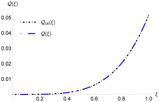
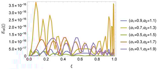
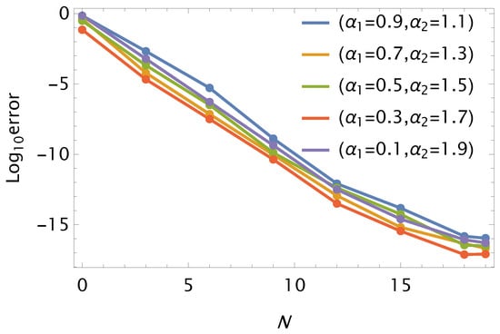
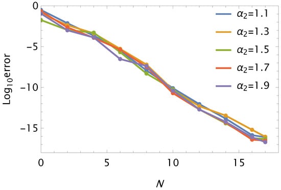
In this problem, the APPSs using RGSJCOMM are calculated for various $N,{\vartheta }_1$, and ${\vartheta }_2$. The resulting error achieves an accuracy of order ${10}^{-17}$ with $N=18$, as shown in Table 1. Comparisons between RGSJCOMM and another method from [35] are presented in Table 2, indicating that RGSJCOMM yields results more accurate than those reported in [35]. Furthermore, Figure 1 and Figure 2 illustrate excellent agreement between $\mathcal{Q}\left(\xi \right)$ and ${\mathcal{Q}}_{18}\left(\xi \right)$ for various values of ${\alpha }_1$ and ${\alpha }_2$ when ${\vartheta }_1={\vartheta }_2=1.5$. Additionally, Figure 3 displays the log-error, demonstrating convergence and the stability of the APPSs for Problem 2 when employing RGSJCOMM.

Table 1. MAE and CPU time (in seconds) for Problem 2 using various $N,{\vartheta }_1,{\vartheta }_1,{\alpha }_1$, and ${\alpha }_2$.

$({\mathit{\alpha }}_1,{\mathit{\alpha }}_2)$	${\mathit{\vartheta }}_1$	${\mathit{\vartheta }}_2$	Errors	0	3	6	9	12	15	18	19
(0.9,1.1)	0	0	$\parallel E_N{\parallel }_{\infty }$	1.19 × 10−01	2.72 × 10−04	3.15 × 10−07	3.15 × 10−10	2.17 × 10−13	2.27 × 10−15	5.16 × 10−17	2.23 × 10−17
			$\parallel E_N{\parallel }_2$	1.11 × 10−01	2.41 × 10−04	3.05 × 10−07	3.12 × 10−10	2.12 × 10−13	2.25 × 10−15	5.02 × 10−17	2.13 × 10−17
			CPU Time	0.119	0.375	0.551	0.715	0.912	1.107	1.312	1.362
	1/2	1/2	$\parallel E_N{\parallel }_{\infty }$	2.29 × 10−01	1.79 × 10−04	2.55 × 10−07	4.25 × 10−10	3.77 × 10−13	3.57 × 10−15	4.66 × 10−17	1.23 × 10−17
			$\parallel E_N{\parallel }_2$	2.19 × 10−01	1.72 × 10−04	2.45 × 10−07	4.20 × 10−10	3.67 × 10−13	3.50 × 10−15	4.61 × 10−17	1.12 × 10−17
			CPU Time	0.125	0.385	0.562	0.727	0.922	1.110	1.320	1.371
	−1/2	−1/2	$\parallel E_N{\parallel }_{\infty }$	3.09 × 10−01	2.59 × 10−04	1.25 × 10−07	3.35 × 10−10	4.17 × 10−13	2.51 × 10−15	6.12 × 10−17	2.43 × 10−17
			$\parallel E_N{\parallel }_2$	3.00 × 10−01	2.42 × 10−04	1.12 × 10−07	3.25 × 10−10	4.10 × 10−13	2.42 × 10−15	6.03 × 10−17	2.33 × 10−17
			CPU Time	0.117	0.361	0.563	0.709	0.909	1.111	1.322	1.353
(0.7,1.3)	1.1	0.5	$\parallel E_N{\parallel }_{\infty }$	2.19 × 10−01	3.42 × 10−04	3.75 × 10−07	4.65 × 10−10	3.32 × 10−13	3.41 × 10−15	3.32 × 10−16	1.63 × 10−16
			$\parallel E_N{\parallel }_2$	2.15 × 10−01	3.32 × 10−04	3.51 × 10−07	4.51 × 10−10	3.21 × 10−13	3.31 × 10−15	3.21 × 10−16	1.51 × 10−16
			CPU Time	0.131	0.395	0.582	0.736	0.930	1.121	1.333	1.370
	0.5	1.1	$\parallel E_N{\parallel }_{\infty }$	3.59 × 10−01	3.51 × 10−04	4.25 × 10−07	3.45 × 10−10	2.61 × 10−13	2.51 × 10−15	4.12 × 10−16	2.73 × 10−16
			$\parallel E_N{\parallel }_2$	3.45 × 10−01	3.40 × 10−04	4.21 × 10−07	3.37 × 10−10	2.52 × 10−13	2.42 × 10−15	4.00 × 10−16	2.64 × 10−16
			CPU Time	0.199	0.401	0.599	0.781	0.960	1.141	1.339	1.387
	1.1	1.1	$\parallel E_N{\parallel }_{\infty }$	4.19 × 10−01	3.32 × 10−04	1.45 × 10−07	5.05 × 10−10	3.66 × 10−13	1.61 × 10−15	3.74 × 10−17	1.62 × 10−17
			$\parallel E_N{\parallel }_2$	4.08 × 10−01	3.22 × 10−04	1.41 × 10−07	4.95 × 10−10	3.55 × 10−13	1.52 × 10−15	3.66 × 10−17	1.42 × 10−17
			CPU Time	0.189	0.382	0.549	0.734	0.937	1.135	1.335	1.402
(0.5,1.5)	0.7	0.7	$\parallel E_N{\parallel }_{\infty }$	2.79 × 10−01	1.62 × 10−04	3.55 × 10−07	4.35 × 10−10	2.36 × 10−13	2.78 × 10−15	2.14 × 10−17	1.65 × 10−17
			$\parallel E_N{\parallel }_2$	2.70 × 10−01	1.45 × 10−04	3.49 × 10−07	4.29 × 10−10	2.31 × 10−13	2.72 × 10−15	2.01 × 10−17	1.61 × 10−17
			CPU Time	0.149	0.409	0.601	0.795	0.961	1.141	1.419	1.412
	0.3	0.3	$\parallel E_N{\parallel }_{\infty }$	3.99 × 10−01	2.82 × 10−04	1.75 × 10−07	2.95 × 10−10	3.98 × 10−13	3.99 × 10−15	4.24 × 10−17	1.45 × 10−17
			$\parallel E_N{\parallel }_2$	3.81 × 10−01	2.67 × 10−04	1.62 × 10−07	2.85 × 10−10	3.91 × 10−13	3.90 × 10−15	4.15 × 10−17	1.40 × 10−17
			CPU Time	0.121	0.380	0.559	0.735	0.936	1.121	1.333	1.392
	1	1	$\parallel E_N{\parallel }_{\infty }$	1.29 × 10−01	3.88 × 10−04	2.79 × 10−07	3.87 × 10−10	2.99 × 10−13	2.29 × 10−15	6.34 × 10−17	2.15 × 10−17
			$\parallel E_N{\parallel }_2$	1.19 × 10−01	3.80 × 10−04	2.71 × 10−07	3.82 × 10−10	2.89 × 10−13	2.20 × 10−15	6.23 × 10−17	2.05 × 10−17
			CPU Time	0.125	0.402	0.592	0.798	0.984	1.115	1.321	1.382
(0.3,1.7)	1	0	$\parallel E_N{\parallel }_{\infty }$	4.19 × 10−01	2.38 × 10−04	3.65 × 10−07	2.77 × 10−10	4.54 × 10−13	3.99 × 10−15	4.21 × 10−16	1.22 × 10−16
			$\parallel E_N{\parallel }_2$	4.07 × 10−01	2.27 × 10−04	3.57 × 10−07	2.67 × 10−10	4.45 × 10−13	3.88 × 10−15	4.11 × 10−17	1.17 × 10−17
			CPU Time	0.130	0.415	0.611	0.801	1.105	1.217	1.422	1.521
	0	1	$\parallel E_N{\parallel }_{\infty }$	1.88 × 10−01	3.58 × 10−04	2.72 × 10−07	3.66 × 10−10	2.41 × 10−13	2.84 × 10−15	5.31 × 10−16	3.42 × 10−16
			$\parallel E_N{\parallel }_2$	1.75 × 10−01	3.51 × 10−04	2.63 × 10−07	3.55 × 10−10	2.39 × 10−13	2.77 × 10−15	5.25 × 10−17	3.37 × 10−17
			CPU Time	0.129	0.388	0.573	0.781	0.966	1.130	1.339	1.382
	1.5	1.5	$\parallel E_N{\parallel }_{\infty }$	3.24 × 10−01	2.72 × 10−04	4.12 × 10−07	2.55 × 10−10	3.87 × 10−13	1.48 × 10−15	3.22 × 10−17	1.22 × 10−17
			$\parallel E_N{\parallel }_2$	3.20 × 10−01	2.66 × 10−04	4.01 × 10−07	2.45 × 10−10	3.78 × 10−13	1.41 × 10−15	3.12 × 10−17	1.13 × 10−17
			CPU Time	0.130	0.403	0.607	0.888	0.990	1.121	1.341	1.377

Table 2. Comparison between RGSJCOMM and the method in [35] for Problem 2 using ${\vartheta }_1={\vartheta }_2=1.5$ and various ${\alpha }_1$ and ${\alpha }_2$.

$({\mathit{\alpha }}_1,{\mathit{\alpha }}_2)$	(0.9,1.1)	(0.7,1.3)	(0.5,1.5)	(0.3,1.7)	(0.1,1.9)
RGSJCOMM ($N=18$)	1.45 × 10−17	1.40 × 10−17	5.31 × 10−17	5.86 × 10−17	4.32 × 10−17
[35] ($N=2048$)	5.39 × 10−11	2.12 × 10−11	2.58 × 10−11	2.75 × 10−11	2.44 × 10−11

Figure 1. APPSs and ExaSs, $\mathcal{Q}\left(\xi \right),{\mathcal{Q}}_{18}\left(\xi \right)$ plots using ${\alpha }_1=0.3,{\alpha }_2=1.7$ and ${\vartheta }_1={\vartheta }_2=1.5$ for Problem 2.

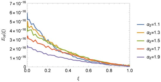
Figure 2. AEs $E_{18}\left(\xi \right)$ plots using ${\vartheta }_1={\vartheta }_2=1.5$ for Problem 2.

Figure 3. Graph of $Lo{g}_{10}(\parallel E_N{\parallel }_{\infty })$ against N using ${\vartheta }_1={\vartheta }_2=1.5$ and various values of ${\alpha }_1$ and ${\alpha }_2$ for Problem 2.

Problem 3.

Consider the BVP [35,36]

$$\left.\begin{array}{c}\stackrel{LC}{0}{\mathbb{D}}_{\xi }^{{\alpha }_2}\mathcal{Q}\left(\xi \right)=-(2\xi +6)D\mathcal{Q}\left(\xi \right)+\mathcal{K}\left(\xi \right),\xi \in (0,1),\hfill \\ \mathcal{Q}\left(0\right)-{\displaystyle \frac{1}{{\alpha }_2-1}}{\mathcal{Q}}^{\prime }\left(0\right)={\mathcal{C}}_1,\mathcal{Q}\left(1\right)+{\mathcal{Q}}^{\prime }\left(1\right)={\mathcal{C}}_2,\hfill \end{array}\right\}$$

(69)

where $\mathcal{K}\left(\xi \right)$ and the constants ${\mathcal{C}}_1,{\mathcal{C}}_2$ are chosen such that the exact solution (ExaS) is $\mathcal{Q}\left(\xi \right)=1+3\xi -7{\xi }^2+4{\xi }^3+{\xi }^4+{\xi }^{{\alpha }_2}+{\xi }^{2{\alpha }_2-1}$. The application of RGSJCOMM gives ${\mathcal{Q}}_N\left(\xi \right)$ in the form

$${\displaystyle {\mathcal{Q}}_N\left(\xi \right)=\sum _{i=0}^N{c}_i{\mathfrak{M}}_i^{({\vartheta }_1,{\vartheta }_2)}\left(\xi \right)+\left(\frac{\left({\alpha }_2+2\right)\left(3{\alpha }_2-2\right)}{2{\alpha }_2-1}\right)\xi +\frac{5{\alpha }_2}{2{\alpha }_2-1}.}$$

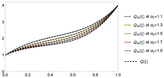
Table 3 illustrates the high efficiency of the $RGSJCOMM$. Additionally, Table 4 compares the approaches from [35,36] with the $RGSJCOMM$, highlighting the latter’s superiority. Figure 4 and Figure 5 display the NUMSs, ${\mathcal{Q}}_{16}\left(\xi \right)$, and error $E_{16}\left(\xi \right)$, respectively, for ${\alpha }_2=1.1,1.3,1.5,1.7,1.9$ using ${\vartheta }_1=1,{\vartheta }_2=0.5$. By showcasing these APPSs and their associated errors, Figure 6 provides a thorough analysis of the performance of $RGSJCOMM$.

Table 3. MAE for Problem 3 using various $N,{\vartheta }_1,{\vartheta }_1$, and ${\alpha }_2$.

${\mathit{\alpha }}_2$	${\mathit{\vartheta }}_1$	${\mathit{\vartheta }}_2$	Errors	0	2	4	6	8	10	12	14	16	17
1.1	0	0	$\parallel E_N{\parallel }_{\infty }$	2.39 × 10−01	1.52 × 10−02	2.25 × 10−04	4.21 × 10−06	1.37 × 10−08	3.25 × 10−10	4.26 × 10−12	1.20 × 10−14	3.33 × 10−16	1.21 × 10−16
			$\parallel E_N{\parallel }_2$	2.31 × 10−01	1.48 × 10−02	2.15 × 10−04	4.14 × 10−06	1.11 × 10−08	3.12 × 10−10	4.17 × 10−12	1.02 × 10−14	3.23 × 10−16	1.15 × 10−16
	1/2	1/2	$\parallel E_N{\parallel }_{\infty }$	3.12 × 10−01	3.72 × 10−02	1.55 × 10−04	5.23 × 10−06	3.57 × 10−08	2.95 × 10−10	2.96 × 10−12	2.27 × 10−14	4.13 × 10−16	7.21 × 10−17
			$\parallel E_N{\parallel }_2$	3.04 × 10−01	3.53 × 10−02	1.44 × 10−04	5.13 × 10−06	3.42 × 10−08	2.64 × 10−10	2.82 × 10−12	2.13 × 10−14	4.02 × 10−16	7.07 × 10−17
	−1/2	−1/2	$\parallel E_N{\parallel }_{\infty }$	4.31 × 10−01	1.81 × 10−02	4.95 × 10−04	6.53 × 10−06	2.28 × 10−08	3.62 × 10−10	3.82 × 10−12	3.77 × 10−14	2.33 × 10−16	1.11 × 10−16
			$\parallel E_N{\parallel }_2$	4.22 × 10−01	1.72 × 10−02	4.79 × 10−04	6.39 × 10−06	2.18 × 10−08	3.41 × 10−10	3.81 × 10−12	3.53 × 10−14	2.22 × 10−16	1.01 × 10−16
1.3	1.1	0.5	$\parallel E_N{\parallel }_{\infty }$	2.51 × 10−01	3.91 × 10−02	2.82 × 10−04	3.43 × 10−06	3.88 × 10−08	1.51 × 10−10	4.92 × 10−12	4.52 × 10−14	3.44 × 10−16	2.23 × 10−16
			$\parallel E_N{\parallel }_2$	2.49 × 10−01	3.88 × 10−02	2.65 × 10−04	3.32 × 10−06	3.77 × 10−08	1.47 × 10−10	4.64 × 10−12	4.32 × 10−14	3.24 × 10−16	8.14 × 10−17
	0.5	1.1	$\parallel E_N{\parallel }_{\infty }$	4.41 × 10−01	1.19 × 10−02	3.28 × 10−04	4.44 × 10−06	2.59 × 10−08	2.98 × 10−10	3.88 × 10−12	2.41 × 10−14	3.14 × 10−16	2.03 × 10−16
			$\parallel E_N{\parallel }_2$	4.30 × 10−01	1.05 × 10−02	3.15 × 10−04	4.22 × 10−06	2.45 × 10−08	2.84 × 10−10	3.76 × 10−12	2.32 × 10−14	3.02 × 10−16	2.99 × 10−16
	1.1	1.1	$\parallel E_N{\parallel }_{\infty }$	1.31 × 10−01	3.23 × 10−02	2.18 × 10−04	1.35 × 10−06	1.45 × 10−08	3.87 × 10−10	2.45 × 10−12	4.25 × 10−14	4.35 × 10−16	2.44 × 10−16
			$\parallel E_N{\parallel }_2$	1.27 × 10−01	3.12 × 10−02	2.01 × 10−04	1.15 × 10−06	1.41 × 10−08	3.74 × 10−10	2.34 × 10−12	4.17 × 10−14	4.26 × 10−16	1.74 × 10−16
1.5	0.7	0.7	$\parallel E_N{\parallel }_{\infty }$	4.01 × 10−01	2.88 × 10−02	1.68 × 10−04	5.74 × 10−06	3.15 × 10−08	2.78 × 10−10	1.65 × 10−12	3.55 × 10−14	5.33 × 10−16	3.14 × 10−16
			$\parallel E_N{\parallel }_2$	3.88 × 10−01	2.78 × 10−02	1.62 × 10−04	5.65 × 10−06	3.06 × 10−08	2.67 × 10−10	1.45 × 10−12	3.29 × 10−14	5.26 × 10−16	2.99 × 10−16
	0.3	0.3	$\parallel E_N{\parallel }_{\infty }$	5.11 × 10−01	3.24 × 10−02	3.99 × 10−04	6.64 × 10−06	4.31 × 10−08	1.68 × 10−10	2.27 × 10−12	4.61 × 10−14	4.73 × 10−16	2.24 × 10−16
			$\parallel E_N{\parallel }_2$	4.89 × 10−01	3.05 × 10−02	3.71 × 10−04	6.51 × 10−06	4.25 × 10−08	1.55 × 10−10	2.21 × 10−12	4.56 × 10−14	4.65 × 10−16	2.20 × 10−16
	1	1	$\parallel E_N{\parallel }_{\infty }$	2.36 × 10−01	2.44 × 10−02	6.56 × 10−04	2.46 × 10−06	2.12 × 10−08	3.82 × 10−10	3.72 × 10−12	2.56 × 10−14	3.64 × 10−16	2.33 × 10−16
			$\parallel E_N{\parallel }_2$	2.25 × 10−01	2.32 × 10−02	6.45 × 10−04	2.36 × 10−06	2.10 × 10−08	3.66 × 10−10	3.68 × 10−12	2.52 × 10−14	3.59 × 10−16	2.27 × 10−16
1.7	1	0	$\parallel E_N{\parallel }_{\infty }$	3.27 × 10−01	4.52 × 10−02	4.26 × 10−04	3.66 × 10−06	1.72 × 10−08	2.92 × 10−10	5.61 × 10−12	1.59 × 10−14	4.24 × 10−16	3.23 × 10−16
			$\parallel E_N{\parallel }_2$	3.19 × 10−01	4.44 × 10−02	4.16 × 10−04	3.60 × 10−06	1.64 × 10−08	2.85 × 10−10	5.46 × 10−12	1.44 × 10−14	4.12 × 10−16	3.01 × 10−16
	0	1	$\parallel E_N{\parallel }_{\infty }$	4.01 × 10−01	3.12 × 10−02	1.06 × 10−04	2.36 × 10−06	4.52 × 10−08	1.82 × 10−10	2.16 × 10−12	2.95 × 10−14	3.50 × 10−16	1.12 × 10−16
			$\parallel E_N{\parallel }_2$	3.88 × 10−01	2.95 × 10−02	8.11 × 10−05	2.15 × 10−06	4.06 × 10−08	1.51 × 10−10	2.03 × 10−12	2.61 × 10−14	3.41 × 10−16	8.02 × 10−17
	1.5	1.5	$\parallel E_N{\parallel }_{\infty }$	1.61 × 10−01	4.41 × 10−02	4.16 × 10−04	3.25 × 10−06	1.99 × 10−08	4.28 × 10−10	1.66 × 10−12	3.81 × 10−14	1.49 × 10−16	1.49 × 10−16
			$\parallel E_N{\parallel }_2$	1.52 × 10−01	4.32 × 10−02	3.99 × 10−04	3.06 × 10−06	1.41 × 10−08	3.98 × 10−10	1.56 × 10−12	3.62 × 10−14	1.28 × 10−16	1.27 × 10−16
1.9	1	0	$\parallel E_N{\parallel }_{\infty }$	5.01 × 10−01	2.61 × 10−02	3.61 × 10−04	1.55 × 10−06	2.91 × 10−08	2.88 × 10−10	2.26 × 10−12	4.51 × 10−14	4.29 × 10−16	2.54 × 10−16
			$\parallel E_N{\parallel }_2$	4.88 × 10−01	2.54 × 10−02	3.44 × 10−04	1.43 × 10−06	2.77 × 10−08	2.65 × 10−10	2.05 × 10−12	4.45 × 10−14	4.13 × 10−16	2.33 × 10−16
	0	1	$\parallel E_N{\parallel }_{\infty }$	2.81 × 10−01	1.72 × 10−02	4.16 × 10−04	2.95 × 10−06	3.85 × 10−08	5.59 × 10−10	1.15 × 10−12	3.61 × 10−14	5.22 × 10−16	3.44 × 10−16
			$\parallel E_N{\parallel }_2$	2.77 × 10−01	1.65 × 10−02	3.98 × 10−04	2.85 × 10−06	3.82 × 10−08	5.49 × 10−10	1.02 × 10−12	3.54 × 10−14	4.99 × 10−16	3.12 × 10−16
	1.5	1.5	$\parallel E_N{\parallel }_{\infty }$	3.11 × 10−01	4.87 × 10−02	2.65 × 10−04	3.56 × 10−06	2.58 × 10−08	2.95 × 10−10	3.25 × 10−12	1.66 × 10−14	2.13 × 10−16	2.13 × 10−16
			$\parallel E_N{\parallel }_2$	2.94 × 10−01	4.78 × 10−02	2.55 × 10−04	3.46 × 10−06	2.44 × 10−08	2.76 × 10−10	3.02 × 10−12	1.56 × 10−14	1.98 × 10−16	2.00 × 10−16

Table 4. Comparison between RGSJCOMM and the methods in [35,36] for Problem 3 using ${\vartheta }_1=1.5,$${\vartheta }_2=0.5$, and various ${\alpha }_2$.

${\mathit{\alpha }}_2$	1.1	1.3	1.5	1.7	1.9
RGSJCOMM ($N=16$)	2.15 × 10−16	1.25 × 10−16	3.31 × 10−16	3.68 × 10−16	2.25 × 10−16
[35] ($N=2048$)	6.91 × 10−05	1.26 × 10−05	1.36 × 10−06	1.22 × 10−06	1.38 × 10−06
[36] ($N=2048$)	1.45 × 10−04	2.36 × 10−05	6.77 × 10−06	3.90 × 10−06	4.00 × 10−06

Figure 4. $\mathcal{Q}\left(\xi \right)$ and ${\mathcal{Q}}_{16}\left(\xi \right)$ plots using ${\alpha }_2=1.1,1.3,1.5,1.7,1.9$ and ${\vartheta }_1=1,{\vartheta }_2=0.5$ for Problem 3.

Figure 5. $E_{16}\left(\xi \right)$ plots using ${\alpha }_2=1.1,1.3,1.5,1.7,1.9$ and ${\vartheta }_1=1,{\vartheta }_2=0.5$ for Problem 3.

Figure 6. Graphs of $Lo{g}_{10}(\parallel E_N{\parallel }_{\infty })$ against N using ${\alpha }_2=1.1,1.3,1.5,1.7,1.9$ and ${\vartheta }_1=1,{\vartheta }_2=0.5$ for Problem 3.

9. Conclusions

In this work, a system of RMGSJ polynomials that satisfies HRBCs has been developed. The use of these polynomials along with the established OMs in the SCM yields APPSs for BVPs (1) and (2). RGSJCOMM was evaluated using three problems, demonstrating the algorithm’s high accuracy and efficiency. We believe that the theoretical findings and the methodology developed herein provide a promising foundation for future research addressing higher-dimensional partial FDEs (such as time-fractional diffusion or wave equations) subject to RBCs.

References

- Baillie, R. Long memory processes and fractional integration in econometrics. J. Econom. 1996, 73, 5–59. [Google Scholar] [CrossRef]
- Mainardi, F. Fractional calculus: Some basic problems in continuum and statistical mechanics. In Fractals and Fractional Calculus in Continuum Mechanics; Springer: New York, NY, USA, 1997. [Google Scholar]
- Chen, W.; Sun, H.; Zhang, X.; Korošak, D. Anomalous diffusion modeling by fractal and fractional derivatives. Comput. Math. Appl. 2010, 59, 1754–1758. [Google Scholar] [CrossRef]
- Hong, D.P.; Kim, Y.M.; Wang, J.Z. A new approach for the analysis solution of dynamic systems containing fractional derivative. J. Mech. Sci. Technol. 2006, 20, 658–667. [Google Scholar] [CrossRef]
- Kaczorek, T. Positive linear systems with different fractional orders. Bull. Pol. Acad. Sci. Tech. Sci. 2010, 58, 453–458. [Google Scholar] [CrossRef]
- Cong, N.; Doan, T.; Tuan, H. Asymptotic stability of linear fractional systems with constant coefficients and small time-dependent perturbations. Vietnam J. Math. 2018, 46, 665–680. [Google Scholar] [CrossRef]
- Mahmudov, N. Approximate controllability of semilinear deterministic and stochastic evolution equations in abstract spaces. SIAM J. Control Optim. 2003, 42, 1604–1622. [Google Scholar] [CrossRef]
- Ahmadova, A.; Mahmudov, N. Existence and uniqueness results for a class of fractional stochastic neutral differential equations. Chaos Soliton Fract. 2020, 139, 110253. [Google Scholar] [CrossRef]
- Huseynov, I.; Mahmudov, N.I. Delayed analogue of three-parameter Mittag-Leffler functions and their applications to Caputo-type fractional time delay differential equations. Math. Method. Appl. Sci. 2024, 47, 11019–11043. [Google Scholar] [CrossRef]
- Bonfanti, A.; Fouchard, J.; Khalilgharibi, N.; Charras, G.; Kabla, A. A unified rheological model for cells and cellularised materials. R. Soc. Open Sci. 2020, 7, 190920. [Google Scholar] [CrossRef]
- Bagley, R.; Torvik, P. Fractional calculus-a different approach to the analysis of viscoelastically damped structures. AIAA J. 1983, 21, 741–748. [Google Scholar] [CrossRef]
- Torvik, P.J.; Bagley, R.L. On the Appearance of the Fractional Derivative in the Behavior of Real Materials. J. Appl. Mech. 1984, 51, 294–298. [Google Scholar] [CrossRef]
- Ahmed, H. Solutions of 2nd-order linear differential equations subject to Dirichlet boundary conditions in a Bernstein polynomial basis. J. Egypt. Math. Soc. 2014, 22, 227–237. [Google Scholar] [CrossRef]
- Izadi, M.; Afshar, M. Solving the Basset equation via Chebyshev collocation and LDG methods. J. Math. Model. 2021, 9, 61–79. [Google Scholar]
- Izadi, M.; Zeidan, D. A convergent hybrid numerical scheme for a class of nonlinear diffusion equations. Comput. Appl. Math. 2022, 41, 318. [Google Scholar] [CrossRef]
- Izadi, M. Numerical approximation of Hunter-Saxton equation by an efficient accurate approach on long time domains. UPB Sci. Bull. Ser. A 2021, 83, 291–300. [Google Scholar]
- Hafez, R.; Youssri, Y. Fully Jacobi–Galerkin algorithm for two-dimensional time-dependent PDEs arising in physics. Int. J. Mod. Phys. C 2024, 35, 2450034. [Google Scholar] [CrossRef]
- Abd-Elhameed, W.; Ahmed, H.; Zaky, M.; Hafez, R. A new shifted generalized Chebyshev approach for multi-dimensional sinh-Gordon equation. Phys. Scr. 2024, 99, 095269. [Google Scholar] [CrossRef]
- Bazhlekova, E. Properties of the fundamental and the impulse-response solutions of multi-term fractional differential equations. Complex Anal. Appl. 2013, 13, 55–64. [Google Scholar]
- Yüzbaşı, Ş.; Izadi, M. Bessel-quasilinearization technique to solve the fractional-order HIV-1 infection of CD4+ T-cells considering the impact of antiviral drug treatment. Appl. Math. Comput. 2022, 431, 127319. [Google Scholar] [CrossRef]
- Abd-Elhameed, W.; Abdelkawy, M.; Alqubori, O.; Atta, A. An accurate tau-based spectral algorithm for the time fractional bioheat transfer model. Bound. Value Probl. 2025, 2025, 124. [Google Scholar] [CrossRef]
- Napoli, A.; Abd-Elhameed, W.M. A new collocation algorithm for solving even-order boundary value problems via a novel matrix method. Mediterr. J. Math. 2017, 14, 170. [Google Scholar] [CrossRef]
- Ahmed, H. Highly Accurate Method for Boundary Value Problems with Robin Boundary Conditions. J. Nonlinear Math. Phys. 2023, 30, 1239–1263. [Google Scholar] [CrossRef]
- Ahmed, H. Highly Accurate Method for a Singularly Perturbed Coupled System of Convection–Diffusion Equations with Robin Boundary Conditions. J. Nonlinear Math. Phys. 2024, 31, 17. [Google Scholar] [CrossRef]
- Abd-Elhameed, W.; Youssri, Y. Spectral solutions for fractional differential equations via a novel Lucas operational matrix of fractional derivatives. Rom. J. Phys. 2016, 61, 795–813. [Google Scholar]
- Balaji, S.; Hariharan, G. An efficient operational matrix method for the numerical solutions of the fractional Bagley–Torvik equation using wavelets. J. Math. Chem. 2019, 57, 1885–1901. [Google Scholar] [CrossRef]
- Ahmed, H. Enhanced shifted Jacobi operational matrices of derivatives: Spectral algorithm for solving multiterm variable-order fractional differential equations. Bound. Value Probl. 2023, 2023, 108. [Google Scholar] [CrossRef]
- Ahmed, H. A New First Finite Class of Classical Orthogonal Polynomials Operational Matrices: An Application for Solving Fractional Differential Equations. Contemp. Math. 2023, 4, 974–994. [Google Scholar] [CrossRef]
- Abd-Elhameed, W.; Ahmed, H. Spectral solutions for the time-fractional heat differential equation through a novel unified sequence of Chebyshev polynomials. Aims Math. 2024, 9, 2137–2166. [Google Scholar] [CrossRef]
- Loh, J.R.; Phang, C. Numerical solution of Fredholm fractional integro-differential equation with Right-sided Caputo’s derivative using Bernoulli polynomials operational matrix of fractional derivative. Mediterr. J. Math. 2019, 16, 28. [Google Scholar] [CrossRef]
- Kilbas, A.; Srivastava, H.; Trujillo, J. Theory and Applications of Fractional Differential Equations; Elsevier: Amsterdam, The Netherlands, 2006; Volume 204. [Google Scholar]
- Szegö, G. Orthogonal Polynomials, 4th ed.; American Mathematical Society: Providence, RI, USA, 1975; Volume XXIII. [Google Scholar]
- Luke, Y. Mathematical Functions and Their Approximations; Academic Press: London, UK, 1975. [Google Scholar]
- Jeffrey, A.; Dai, H. Handbook of Mathematical Formulas and Integrals, 4th ed.; Elsevier: Amsterdam, The Netherlands, 2008. [Google Scholar]
- Kim, H.; Lee, J.; Jang, B. An efficient numerical approach for solving two-point fractional order nonlinear boundary value problems with Robin boundary conditions. Adv. Differ. Equ. 2021, 2021, 193. [Google Scholar] [CrossRef]
- Cen, Z.; Huang, J.; Xu, A. An efficient numerical method for a two-point boundary value problem with a Caputo fractional derivative. J. Comput. Appl. Math. 2018, 336, 1–7. [Google Scholar] [CrossRef]
Disclaimer/Publisher’s Note: The statements, opinions and data contained in all publications are solely those of the individual author(s) and contributor(s) and not of MDPI and/or the editor(s). MDPI and/or the editor(s) disclaim responsibility for any injury to people or property resulting from any ideas, methods, instructions or products referred to in the content. |
© 2025 by the author. Licensee MDPI, Basel, Switzerland. This article is an open access article distributed under the terms and conditions of the Creative Commons Attribution (CC BY) license (https://creativecommons.org/licenses/by/4.0/).