Deep Brain Tumor Lesion Classification Network: A Hybrid Method Optimizing ResNet50 and EfficientNetB0 for Enhanced Feature Extraction

Abstract

Brain tumors usually appear as masses formed by localized abnormal cell proliferation. Although complete removal of tumors is an ideal treatment goal, this process faces many challenges due to the aggressive nature of malignant tumors and the need to protect normal brain tissue. Therefore, early diagnosis is crucial to mitigate the harm posed by brain tumors. In this study, the classification accuracy is improved by improving the ResNet50 model. Specifically, the image is preprocessed and enhanced firstly, and the image is denoised by fractional calculus; then, transfer learning technology is adopted, the ECA attention mechanism is introduced, the convolutional layer in the residual block is optimized, and the multi-scale convolutional layer is fused. These optimization measures not only enhance the model’s ability to grasp the overall details but also improve its ability to recognize micro and macro features. This allows the model to understand data features more comprehensively and process image details more efficiently, thereby improving processing accuracy. In addition, the improved ResNet50 model is combined with EfficientNetB0 to further optimize performance and improve classification accuracy by utilizing EfficientNetB0’s efficient feature extraction capabilities through feature fusion. In this study, we used a brain tumor image dataset containing 5712 training images and 1311 validation images. The optimized ResNet50 model achieves a verification accuracy of 98.78%, which is 3.51% higher than the original model, and the Kappa value is also increased by 4.7%. At the same time, the lightweight design of the EfficientNetB0 improves performance while reducing uptime. These improvements can help diagnose brain tumors earlier and more accurately, thereby improving patient outcomes and survival rates.

1. Introduction

Brain tumors are among the most destructive and life-threatening malignant nervous system tumors. They have high incidence and mortality rates. These tumors severely impact patient health [1,2]. Due to the rapid growth of tumor cells, thousands of people die every year [3]. Surgical removal of brain tumors is a crucial treatment method. However, due to the complexity of brain tissue and the unique growth patterns of tumors, achieving complete resection presents numerous challenges. Therefore, accurate and rapid identification of brain tumors is critical for planning treatment, predicting disease direction, and tracking outcomes [4,5]. In the process of classifying brain tumors, the symmetrical or asymmetrical nature of the tumor serves as a crucial basis for diagnosis. From a morphological standpoint, tumors with symmetrical features are usually categorized as benign or low-grade. In contrast, tumors with asymmetrical features are more often identified as high-grade malignancies. Specifically, symmetrical tumors generally exhibit slow growth and a lower likelihood of dissemination within the brain. Magnetic resonance imaging (MRI) is a medical examination technique, which uses magnetic fields and radio waves to generate images of the body’s internal structures. It produces detailed images by detecting the reaction of water molecules in the human body in a strong magnetic field. It plays a crucial role in detecting and diagnosing brain tumors and aids physicians in clearly identifying the location, size, and nature of the tumors [6,7]. Currently, MRI stands out as the premier approach for early identification of brain tumors in clinical diagnosis [8]. However, the method of manual judgment is often due to too few experienced doctors and too many patients, which is prone to misjudgment and missed judgment [9]. The study examines four types of brain tumor lesions: glioma, meningioma, no tumor, and pituitary. Glioma is a highly malignant tumor that originates from the brain’s glial cells and typically has a poor prognosis. Meningioma is a benign tumor that originates from the meninges, characterized by slow growth and the potential to compress brain tissue. The “no tumor” category indicates the absence of any tumor. Pituitary tumors originate from the pituitary gland and are mostly benign. These four types of brain tumors are depicted in Figure 1.

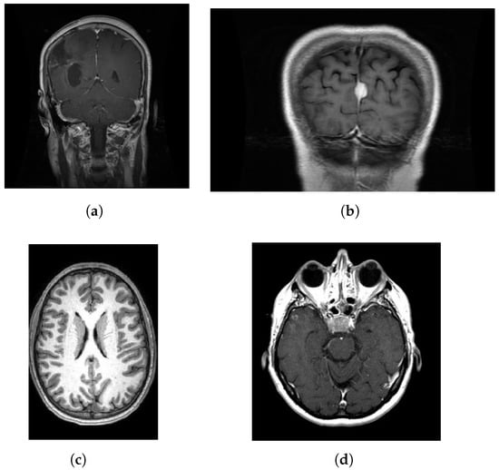
Figure 1. Four types of brain tumors exist: (a) glioma, (b) meningioma, (c) no tumor, and (d) pituitary.

In recent times, the advent of computer-aided diagnosis (CAD) technology, particularly deep learning approaches, has revolutionized clinical image interpretation and disease diagnosis [10]. The reason is that convolutional neural networks (CNNs) can autonomously detect intricate patterns in images and accurately identify lesions with their powerful feature extraction capabilities. With the help of multi-layer convolution and pooling operations, CNNs analyze images layer by layer, extracting features from basic local details to more complex, high-level representations. Ultimately, they accomplish the classification task through the fully connected layer [11].

For example, in breast tumor classification tasks, CNNs significantly outperform traditional methods with their strong feature extraction capabilities [12]. In the classification task of diabetic retinopathy (DR), Ref. [13] employs a multi-step approach. First, fractal analysis is used to identify the chaotic characteristics of fundus images. Next, features are extracted using two-dimensional steady-state wavelet transformation. Key features are then screened using chaotic particle swarm optimization combined with KNN. Finally, the classification is completed using a recurrent neural network with long short-term memory.

Owing to the robust feature extraction capacity of CNNs, these networks have found extensive application in brain tumor classification tasks [14,15]. For instance, Ref. [16] introduced the CerebralNet architecture, which uses MobileNetV2 as its backbone and integrates an Atrous module to enhance feature extraction. This architecture also incorporates a probability-enhanced strategy to simulate artifacts, achieving over 91% accuracy in the original dataset (BM) and 96% in the enhanced dataset (ABM). This makes it a highly effective method for brain tumor detection. To address the limited feature extraction ability of single deep learning architectures in brain tumor classification, Ref. [17] proposed a hybrid model framework (FCBTC) based on feature splicing. By fusing the feature vectors of three pre-trained models—ResNet50, VGG16, and DenseNet121—the model’s ability to capture complex patterns is enhanced, thereby improving classification performance. Ref. [18] proposes a multitask CNN for predicting overall survival (OS) in patients with glioblastoma (GBM) from preoperative multimodal MRI data. This method significantly improves prediction accuracy by simultaneously predicting tumor genotype and OS. Ref. [19] proposes a novel framework leveraging transfer learning to achieve high-accuracy classification of brain tumors in MRI images. Evaluations with pre-trained architectures like ResNet, AlexNet, and VGG16 show that the enhanced ResNet 50 model attains 99.30% and 98.40% precision in classifying benign and malignant tumors, respectively. These results surpass existing techniques, enhancing image fusion quality and facilitating more accurate diagnoses. Lastly, Ref. [20] uses the YOLO NAS model to detect and classify pituitary tumors, meningiomas, gliomas, and non-neoplastic tumors from MRI images of brain tumors. The study utilizes the Rembrandt Repository’s MRI image database, preprocessing images with hybrid anisotropic diffusion filtering (HADF) and segmenting them using U-Net and EfficientNet-based encoder–decoder networks (En–DeNet). The final classification model is developed using YOLO NAS technology.

Attention mechanisms can be used in computer vision tasks to capture fine-grained features and are widely used in image classification. For example, Ref. [21] proposes a cross-amplified attention mechanism named CroMAM to forecast the genetic profile and survival prognosis of glioma. The model uses Swin Transformer and Vision Transformer to extract features by fusing multi-magnification information and designs a cross-magnification attention analysis method to improve interpretability. The experimental results indicate that the model demonstrates outstanding performance in the prediction task. Ref. [22] proposed a Transformer model calles ConvAttenMixer, which combines a convolutional layer and two attention mechanisms (self-attention and external attention) for brain tumor MRI image classification. The experiments show that ConvAttenMixer outperforms other baselines, and the accuracy can be improved by about 4.7% compared with the accuracy of the baseline. Ref. [23] introduces a brain tumor MRI classification framework leveraging a dual-branch global–local parallel architecture, integrating macroscopic context and detailed features. Categorical attention blocks are incorporated to address sample imbalance. The evaluation outcomes reveal that the micro-average AUC reaches 0.989, surpassing several established pre-trained CNN architectures, thereby validating the efficacy of the proposed approach.

While CNN technology has advanced notably in recent times, with its classification accuracy improving, this progress is not without its cost. Specifically, with the increase in network structure complexity and the substantial rise in model parameter count, the runtime of CNN models also shows a marked upward trend. This phenomenon not only poses a challenge to application scenarios with high real-time requirements but also limits its widespread deployment in resource-constrained computing environments to a certain extent. Therefore, how to effectively optimize the running efficiency of models while maintaining high accuracy has become one of the central challenges in the domain of deep learning [24]. To aid in the early detection and classification of tumors, Ref. [25] utilizes a pre-trained GoogLeNet to extract features from brain MRI images and applied softmax, SVM, and K-NN classifiers for classification. The method has been validated on multiple datasets, proving that the training speed and accuracy are far superior to existing models. Ref. [26] introduces a hierarchical classification framework for brain tumor images, integrating EfficientNet and a multi-head attention network. This framework employs a pre-trained EfficientNetB4 for feature extraction, refines features via multi-route convolution, and concludes with classification using a fully connected dual-dense network. The model achieves excellent accuracy and running speed on the TCIA dataset, which is better than the EfficientNetB4 model. Ref. [27] introduces the MK-YOLOv8 framework, a compact deep learning architecture for real-time identification and categorization of brain tumors in MRI imagery. The model integrates lightweight convolutions and modules like Ghost convolution and C3Ghost to boost feature extraction efficacy, lower computational demands, and augment the detection of small tumors.

In addition to incorporating attention mechanisms, lightweight modules, and transfer learning to enhance model effectiveness, brain tumor images often exhibit challenges such as suboptimal visual clarity and significant scale variations. Addressing these issues, image preprocessing is conducted using the canonical ResNet50 architecture. Specifically, an enhanced attention module is integrated to substitute the standard 3 × 3 convolution in the residual framework of the adapted ResNet50, and multi-scale convolution is incorporated into the residual pathway. This modification transforms the residual pathway from a straightforward linear mapping to a more intricate feature extraction process, thereby boosting the model’s training performance metrics. The main improvements are as follows:

(1)

The quality of the pictures is improved so that the model can better deal with the phenomenon of uneven pictures in the brain tumor dataset.

(2)

The performance index of the model is enhanced through the application of an ECA module and multi-scale convolution, and the expression capability of the model is enriched by optimizing the residual connection.

(3)

Improve model training efficiency, improve accuracy, and shorten training time.

The remainder of the manuscript is structured as follows. Section 2 introduces the research methods used for brain tumor classification. The study utilizes a public dataset containing MRI images of four types of brain tumors, and the images undergo preprocessing and augmentation. In terms of the model, optimization is based on ResNet50, incorporating the ECA attention mechanism, multi-scale convolution, and fractional calculus denoising, along with feature fusion with EfficientNetB0 to enhance performance. Additionally, transfer learning techniques are employed, with detailed explanations of evaluation metrics and hyperparameter settings. In Section 3, some definitions of Grünwald–Letnikov Fractional Derivative and the denoising effect of this method and the existing method are provided. Section 4 presents the experimental results obtained from optimizing the ResNet50 model in conjunction with the EfficientNetB0 model for the brain tumor classification task, including improvements in performance metrics, the effects of different optimization modules, and visual analysis of the models. Section 5 discusses the reasons for the performance improvements after model optimization and fusion, including contributions from the ECA attention mechanism, multi-scale convolution, transfer learning, and EfficientNetB0, as well as the limitations of the model and future research directions. Section 6 covers the conclusion.

2. Materials and Methods

2.1. Materials

In the current research, brain tumor images are derived from two existing public datasets on Kaggle, the Brain Tumor MRI dataset and the Brain Tumor Classification dataset (MRI), provided by multiple medical institutions, and the download links are https://www.kaggle.com/datasets/masoudnickparvar/brain-tumor-mri-dataset/data (accessed on 1 January 2021) and https://www.kaggle.com/datasets/sartajbhuvaji/brain-tumor-classification-mri (accessed on 1 August 2025). The dataset comprises dual-modality high-definition images captured via MRI, encompassing four classifications: glioma, meningioma, no tumor, and pituitary. In the Brain Tumor MRI dataset, there are 300 images of glioma, 306 images of meningioma, 405 images of notumor, and 300 images of pituitary. In the Brain Tumor Classification dataset, there are 100 images of glioma, 115 images of meningioma, 105 images of notumor, and 74 images of pituitary. The total image numbers of Brain Tumor MRI dataset and Brain Tumor Classification dataset are 1311 and 394, respectively, and the details are given in Table 1.

Table 1. Raw brain tumor dataset.

Category	Brain Tumor MRI Dataset	Brain Tumor Classification	Total
glioma	300	100	400
meningioma	306	115	421
notumor	405	105	510
pituitary	300	74	374
Total	1311	394	1705

2.2. Methods

The main goal of this paper is to utilize the ResNet50 deep learning model for early brain tumor detection [28] and to enhance the model’s precision and computational efficiency through network structure modifications, transfer learning, and integration of the EfficientNetB0 lightweight module. However, the original medical images have problems such as asymmetric image size, poor image quality, and insufficient contrast, which lead to the inability to directly feed the images to the model or affect the training performance of the model. In addition, brain tumor datasets are often limited in number; as shown in Table 1, two datasets are selected but only 1705 images are selected, resulting in the model being susceptible to overfitting and the validation performance being diminished. The workflow of the brain tumor identification framework is depicted in Figure 2, which includes five steps as image selection, categories of brain tumors, image preprocessing, model training, and model evaluation.

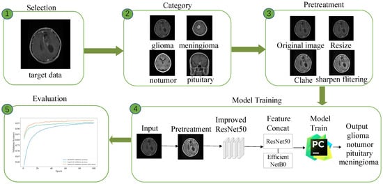
Figure 2. Comprehensive flowchart of the brain tumor identification framework.

2.2.1. Picture Preprocessing

As depicted in Figure 1, due to the asymmetric image size of the kaggle dataset, the image details are not clear, and image preprocessing is required. The dataset itself is an off-white image, so there is no need to grayscale the image. For the asymmetry of the original image size and the large resolution of some images, it not only occupies a large space but also leads to slow model training, so the image size is uniformly adjusted to 224 × 224 [29]. Brain tumor images under MRI imaging have become a core means of analyzing and diagnosing tumor pathological features [30]. Since MRI images can have low contrast, especially between the brain tumor area and surrounding normal tissue, using Clahe equalization can enhance the local contrast of the image, making the tumor’s boundaries and internal structures clearer [31]. In order to clearly present the details of tumor boundaries and blood vessels in MRI brain tumor images, highlight the differences between the lesion area and normal tissue, facilitate doctors to diagnose more accurately, and optimize the diagnostic efficacy of the automated detection system, Laplace sharpening filtering is utilized to augment the image quality. The pre-processed image is depicted in Figure 3.

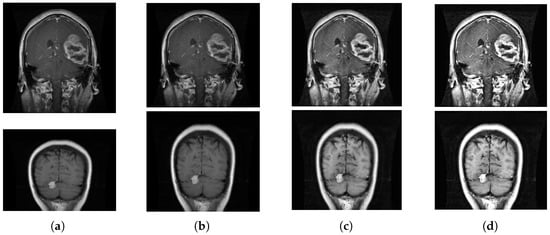
Figure 3. Picture preprocessing: (a) original picture, (b) picture resize, (c) picture clahe equalization, and (d) picture Laplace sharpening filter.

As you can see from Table 1, even if two different datasets are integrated, the total number is still small, necessitating image augmentation. This paper employs several image expansion strategies. Initially, the dataset is augmented by applying random rotations and translations to the images, as well as adjusting the brightness of the pictures. However, the overuse of these techniques may result in excessive conformity to training data, thereby reducing the model’s ability to generalize. To address this, some novel augmentation techniques such as CUTOUT, MIXUP, and Local Augment are used. The original dataset is split into training and validation sets, and the dataset is enriched by a variety of image augmentation strategies. Table 2 lists the expanded brain tumor dataset. The expanded picture is depicted in Figure 4.

Table 2. Brain tumor dataset following picture augmentation.

Category	Training Set	Validation Set	Total
glioma	1321	300	1621
meningioma	1339	306	1645
notumor	1595	405	2000
pituitary	1457	300	1757

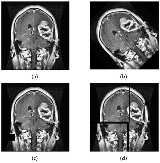
Figure 4. Picture extension: (a) initial picture, (b) picture flip, (c) picture cropping, and (d) local augment.

As depicted in Figure 4, (a) is the original image of the pre-processed MRI, (b) is the MRI image randomly flipped between [−180°–180°], (c) fills in the 0 pixel value of 1 × 1 to cut off part of the area in the MRI, and (d) crops the image into four parts, and each part applies a different image enhancement technique. By applying different image enhancement techniques to increase the variety of images, we avoid overfitting images and improve the generalization ability.

2.2.2. Fractional Calculus Denoising

In the field of image processing, fractional calculus has become an indispensable technical means in key links such as denoising, edge detection, and feature extraction due to its excellent performance [32]. It realizes the precise control of complex image structure and noise by using non-integer derivatives and integration operations. In this study, the Grünwald–Letnikov integral is employed to achieve fractional calculus denoising to improve the presence of noise in the image. The Grünwald–Letnikov definition is shown below.

3. Grünwald–Letnikov Fractional Derivative

• In traditional calculus, first-order derivatives are approximated by differences. For a function $f\left(t\right)$, its first-order derivative can be expressed as

  $$f^{\left(1\right)}\left(t\right)=\underset{h\to 0}{lim}{\displaystyle \frac{f\left(t\right)-f(t-h)}{h}},$$

  (1)

  where $f^{\left(1\right)}\left(t\right)$ represents the first-order derivative of the function $f\left(t\right)$ at point t, and h is the differential step. This definition approximates the rate of change of the function at point t by calculating the difference between the function value at point t and its neighbor point $t-h$ and dividing this difference by the distance h between the two points. This differential method is widely used in numerical calculations due to its simplicity and efficiency.
• For higher-order derivatives, the above definitions can be extended. For a function $f\left(t\right)$, its n-th order derivative can be expressed as

  $$f^{\left(n\right)}\left(t\right)=\underset{h\to 0}{lim}{\displaystyle \frac{1}{h^n}}\sum _{k=0}^n{(-1)}^k\left({\displaystyle \genfrac{}{}{0pt}{}{n}{k}}\right)f(t-kh),$$

  (2)

  where $f^{\left(n\right)}\left(t\right)$ is the n-th order derivative of $f\left(t\right)$, h is the step size, and $\left({\displaystyle \genfrac{}{}{0pt}{}{n}{k}}\right)$ is the binomial coefficient.
• Binomial coefficient is defined as

  $$\left({\displaystyle \genfrac{}{}{0pt}{}{n}{k}}\right)={\displaystyle \frac{n(n-1)(n-2)\cdots (n-k+1)}{k!}},$$

  (3)

  where $\left({\displaystyle \genfrac{}{}{0pt}{}{n}{k}}\right)$ is the binomial coefficient, n is the order of the derivative, and k is the index of summation. It expresses the number of combinations of k elements selected from n elements. In the definition of derivatives, binomial coefficients are used to assign weights to each point, allowing for a more accurate approximation of higher-order derivatives.
• The Grünwald–Letnikov fractional derivative is a method of approximating fractional order derivatives by differential. It is based on the following definitions:
  • Left-sided fractional derivative:

    $${}_a{}^{G}D_t^{\alpha }f\left(t\right)=\underset{h\to 0^{+}}{lim}{\displaystyle \frac{1}{h^{\alpha }}}\sum _{k=0}^{⌊{\displaystyle \frac{t-a}{h}}⌋}{(-1)}^k\left({\displaystyle \genfrac{}{}{0pt}{}{\alpha }{k}}\right)f(t-kh),$$

    (4)

    where ${}_a{}^{G}D_t^{\alpha }f\left(t\right)$ is the left-sided $\alpha$-th order Grünwald–Letnikov fractional derivative of $f\left(t\right)$, a is the lower limit of the derivative, h is the step size, and $⌊·⌋$ denotes the floor function. This definition is based on generalized binomial coefficients assigning weights to different points, approximating the fractional order change rate of the function by calculating the multi-point difference value, and the left-end fractional order derivative focuses on the behavior to the left of point t.
  • Right-sided fractional derivative:

    $${}_t{}^{G}D_b^{\alpha }f\left(t\right)=\underset{h\to 0^{+}}{lim}{\displaystyle \frac{1}{h^{\alpha }}}\sum _{k=0}^{⌊{\displaystyle \frac{b-t}{h}}⌋}{(-1)}^k\left({\displaystyle \genfrac{}{}{0pt}{}{\alpha }{k}}\right)f(t+kh),$$

    (5)

    where ${}_t{}^{G}D_b^{\alpha }f\left(t\right)$ is the right-sided $\alpha$-th order Grünwald–Letnikov fractional derivative of $f\left(t\right)$, b is the upper limit of the derivative, h is the step size, and $⌊·⌋$ denotes the floor function. The right-end fractional derivative is similar to the left-end fractional derivative, but in the opposite direction, and is primarily concerned with the behavior of the function to the right of the t-point.
• Laplace transform:
  • When $\alpha \in [0,1)$,

    $$\mathcal{L}\left[{}_0{}^{G}D_t^{\alpha }f\left(t\right)\right]=s^{\alpha }F\left(s\right),$$

    (6)

    where $\mathcal{L}$ denotes the Laplace transform, s is the complex frequency variable, and $F\left(s\right)$ is the Laplace transform of $f\left(t\right)$. Laplace transforms are an important tool for analyzing fractional derivatives.
  • When $\alpha >1$, the Laplace transform does not exist.

In the Grünwald–Letnikov definition of fractional derivatives, fractional derivatives are approximated by a weighted sequence of differences. The weights in this differential sequence are determined by the generalized binomial coefficients $\left({\displaystyle \genfrac{}{}{0pt}{}{\alpha }{k}}\right)$. These weights can actually be seen as a kind of “integral weight” because they act like integrals in calculations. Specifically, the calculation process of fractional derivatives can be seen as the weighted summation of the values of the function $f\left(t\right)$ at different points, and the distribution of these weights is similar to that of integral kernels.

In this way, the fractional derivative contains not only the properties of differentiation (approximating the derivative by difference) but also the property of integration (smoothing the signal by weighted summing). This combination allows fractional derivatives to process both high-frequency and low-frequency components of signals, excelling in denoising and feature extraction.

The image of Grünwald–Letnikov after denoising is shown in Figure 5.

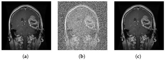
Figure 5. Picture extension: (a) initial picture, (b) noise picture, and (c) noise cancellation picture.

The denoising effects of bilateral filtering and Gaussian filtering are shown in Figure 6.

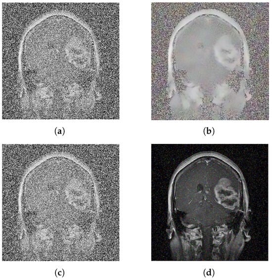
Figure 6. Denoise image: (a) noise picture, (b) bilateral filtered image, (c) noise picture, and (d) Gaussian filtered image.

As can be seen from the above Figure 6, the denoising effect of bilateral filtering is not very good. Although Gaussian filtering is effective in denoising, there are still some noises. In contrast, the denoising effect of fractional calculus is better.

3.1. Model Structure

The advantage of selecting the ResNet50 architecture is its superior performance and computational efficiency [33]. ResNet50 addresses issues related to vanishing and exploding gradients in deep network training via residual connections, enabling the network to capture more intricate feature representations and thereby significantly enhancing the model’s precision and adaptability. Additionally, ResNet50 demonstrates strong performance on multiple benchmark datasets, possesses robust transfer learning capabilities, and can rapidly acclimate to diverse tasks and datasets. Consequently, this study utilizes ResNet50 as the core framework, with the ResNet50 framework illustrated in Figure 7.

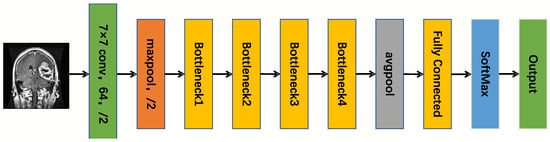
Figure 7. The ResNet50 framework.

In Figure 7, 7 × 7 denotes the size of the convolutional kernel, maxpool stands for maximum pooling layer, /2 signifies that the stride length is 2, Bottleneck represents bottleneck residual structure, and avgpool stands for average pooling layer. The ResNet50 architecture comprises several key components. Initially, the input layer receives a picture with dimensions 224 × 224 × 3. This picture first undergoes a 7 × 7 convolutional layer with a stride length of 2, producing 64 output channels. Subsequently, it is processed by a 3 × 3 max-pooling layer, which is a stride of 2 for dimensionality reduction. After downsampling, it passes through four residual blocks; each residual block contains multiple residual units, and each residual element is composed of three layers of convolution, specifically a 1 × 1 convolution. This architecture employs a 3 × 3 convolution for reducing the number of dimensions, while a 1 × 1 convolution is utilized for extracting features and expanding the dimensionality. After the final residual block, a global average pooling layer is applied to compress the feature map into a fixed-size vector by lowering its dimensions. This vector is subsequently fed into a fully connected layer, where the output size aligns with the number of classes in the classification task. Eventually, the output from the fully connected layer is processed through a Softmax function to generate classification probabilities. The two ResNet50 residual structures are shown in Figure 8.

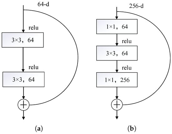
Figure 8. Residual configurations: (a) regular residual configuration and (b) bottleneck residual configuration.

Figure 8a and Figure 8b show two different residual configurations: Basic residual configurations and Bottleneck residual configurations, respectively. Both configurations are core components of ResNet and are used to build networks at different depths. The base residual block contains two convolutional layers with a 3 × 3 kernel, each followed by a nonlinear activation function. The residual connection then adds the input directly to the output of the convolutional layer and then activates the function through a nonlinear operation. The residuals of the bottleneck residual structure are connected in the same way as the basic residual block, and the convolutional layer includes three convolutional layers, two convolutional layers with a 1 × 1 kernel and one convolutional layer with a 3 × 3 kernel. Both residual structures require a 1 × 1 convolution to restore the original channel count because a 1 × 1 convolution provides channel alignment for residual connections and other structures, ensuring that the feature maps of different branches can be added correctly. The 1 × 1 convolution enhances feature expression ability while maintaining the channel count.

3.2. Model Improvements

Self-attention is a technique that allows the model to dynamically analyze the correlation between elements of the input sequence. It generates feature representations with contextual information by calculating the associative weight of each element in relation to the others. The mechanism first converts the input into a query, key, and value vector, then assesses the affinity between the query and the key to determine a weighting factor, and ultimately applies this weight to the fusion value vector. This design is capable of capturing both nearby and distant dependencies, avoiding the sequential computation limitations of RNNs, and has become the core module of Transformer, widely used in the field of deep learning [34]. The equation for the self-attention process is presented below.

$$A=\mathrm{softmax}\left(Q{K}^{\mathsf{T}}\right),$$

(7)

$$F_{\mathrm{out}}=AV.$$

(8)

In Equation (7), the symbols Q, K, and T correspond to the query, key, and transpose operations, respectively. Formula $A=\mathrm{softmax}\left(Q{K}^{\mathsf{T}}\right)$ calculates the query matrix Q and the transposed key matrix $K^{\mathsf{T}}$. The attention score is then normalized by the softmax function to obtain the attention matrix A. In Equation (8), V denotes the value. $F_{\mathrm{out}}$ represents the final output feature matrix of the self-attention mechanism. The self-attention mechanism functions by transforming the input into three components: query, key, and value matrices. These components are derived through linear transformations. The attention scores are computed by taking the dot product of the query and key matrices, which results in an attention matrix. This matrix is then utilized to weight the value matrix, producing the final output of the self-attention mechanism.

Nevertheless, despite its proficiency in modeling global relationships, self-attention demands extensive data support and incurs high costs for structural modifications, rendering it unsuitable for the small-scale dataset in this study. At the 2020 CVPR conference, a new attention mechanism is proposed: the ECA attention mechanism. Compared with the self-attention mechanism, the ECA attention mechanism dynamically calibrates the importance of the channel through lightweight channel attention mechanisms (such as 1D convolution or cross-channel interaction), which directly enhances the model’s capacity to discern details. Moreover, the ECA module is better adapted to computer vision applications like image categorization and is more accommodating to limited data compared to the self-attention mechanism. The equation for the ECA attention mechanism is presented below.

$$g\left(x\right)={\displaystyle \frac{1}{H\times W}}\sum _{i=1}^H\sum _{j=1}^W{X}_{i,j}\in {\mathbb{R}}^C,$$

(9)

$$k={∥{\displaystyle \frac{{log}_2\left(C\right)}{\gamma }}+{\displaystyle \frac{b}{\gamma }}∥}_{\mathrm{odd}},$$

(10)

$$z=f_k\left(g\left(x\right)\right)=\sigma \left(W\ast \delta (W^{\prime }\ast g\left(x\right))\right),$$

(11)

$$Y=X\odot \sigma \left(z\right).$$

(12)

In Equation (9), C denotes the channel count of the input data, while H and W correspond to the spatial dimensions (height and width) of the data. $X_{i,j}$ indicates the values of the data X at positions $(i,j)$, and $g\left(x\right)$ represents the output after applying global average pooling. Equation (9) describes a global average pooling (GAP) operation whose purpose is to compress the spatial dimensions (height H and width W) of each channel of the input feature graph X into a single value, resulting in the global descriptor $g\left(x\right)$ for each channel. In Equation (10), Y and b represent the hyperparameters used to control the calculation of the size of the convolutional kernels. ${log}_2$ denotes the logarithm function with base 2. The logarithm function ${log}_2\left(C\right)$ computes the logarithm of C to base 2. This operation is commonly used for scaling or normalizing data. ${∥·∥}_{\mathrm{odd}}$ represents the closest odd number as the convolutional kernel size usually needs to be odd. The goal of Equation (10) is to dynamically determine the kernel length k for the 1D convolution according to the channel count C of the input data. This avoids manually resizing convolutional cores. In Equation (11), $f_k\left(g\left(x\right)\right)$ represents the kth feature extraction function applied to input $g\left(x\right)$. Here, $g\left(x\right)$ is the input feature, and $f_k$ is a function used to extract a specific feature representation from the input feature. $W^{\prime }$ is the weight parameter of the one-dimensional convolution, $W^{\prime }\ast g\left(x\right)$ represents a one-dimensional convolution operation on $g\left(x\right)$ to generate an intermediate feature $\delta (W^{\prime }\ast g\left(x\right))$, and $\delta$ represents the activation function and is used to introduce nonlinearity. Equation (11) describes a one-dimensional convolutional operation in the ECA attention mechanism to generate channel attention weights z. In Equation (12), X is the input matrix, and Y is the output matrix. $\sigma \left(z\right)$ is the channel attention weight normalized by the Sigmoid activation function, and ⊙ represents element-wise multiplication operations. This means that each pixel value for each channel is multiplied by the corresponding channel attention weight. Equation (12) describes how to adjust the original feature map X using the channel attention weight z; important features can be enhanced and unimportant features can be suppressed by channel attention weight $\sigma \left(z\right)$. Therefore, in order to optimize the performance of the proposed model, the standard convolutional layer in the residual module is replaced by the ECA attention module. This substitution addresses the limitations of the self-attention mechanism when dealing with limited data and improves the model’s ability to handle fine-grained details. The design of residual blocks aims to effectively mitigate issues related to vanishing gradients and network degradation in deep neural networks. By incorporating residual branches, the network is able to focus on learning the differences between the input and output (i.e., the residuals) instead of attempting to learn the entire mapping relationship directly. The fundamental structure of the residual module is as follows:

$$y=F\left(x\right)+x,$$

(13)

where $F\left(x\right)$ is a feature extractor function, x represents the input data, and y indicates the resulting feature. This design not only helps alleviate the vanishing gradient problem in deep networks but also ensures that even when the output $F\left(x\right)$ approaches zero, the input data x can still be fully passed to the next layer, thus maintaining the flow of information and learning capabilities in the network. Nevertheless, in certain scenarios, $F\left(x\right)$ might fail to effectively extract meaningful features, and its output could even approach zero. When this occurs, the resultant feature y of the residual block is largely dictated by the input data x, with $F\left(x\right)$ making a minimal contribution. This, in turn, prevents $F\left(x\right)$ from achieving its maximum effectiveness. To tackle this challenge, multi-scale convolution is introduced into the residual branch as a substitute for the traditional single-path feature extraction method. Multi-scale convolution captures information across different scales of the input features by employing convolutional kernels of various sizes in parallel, such as 1 × 1, 3 × 3, and 5 × 5. Specifically, the single-layer convolution primarily serves to regulate the channel dimensions and facilitate channel-wise dimensionality expansion or reduction. The 3 × 3 convolution focuses on extracting local features, while the 5 × 5 convolution, due to its larger receptive field, captures global contextual information and long-range dependencies in images. The core advantage of multi-scale convolution is that it can significantly improve the network’s modeling ability of complex visual patterns by fusing the features of different receptive fields in parallel. Once the multi-scale feature processing is finished, the outputs from the multi-scale convolutions are combined along the channel axis using the concat operation, merging features from various receptive fields. Subsequently, a 1 × 1 convolution is applied to compress the concatenated high-dimensional features, ensuring they align with the channel count required by the following network layers. This design ensures that even when the $F\left(x\right)$ output is nearly negligible, the multi-scale feature extraction layer can capture valuable features across various scales, thereby enriching the feature details. The improved residual connection is depicted in Figure 9.

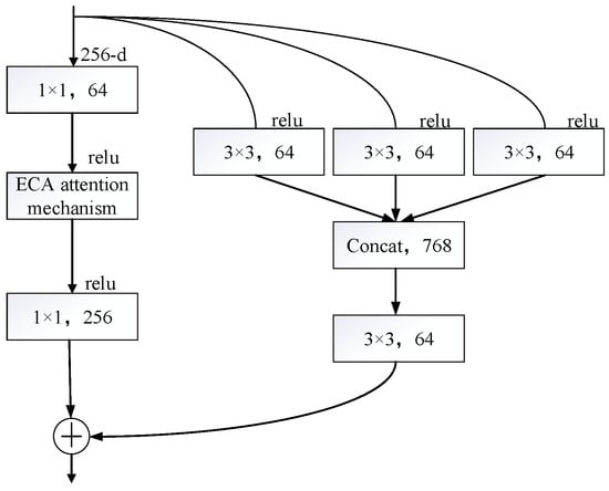
Figure 9. Residual structure optimization.

Through the incorporation of multi-scale convolution, the network is capable of concurrently extracting multi-scale information from input features, thereby significantly boosting its ability to model complex visual patterns. Convolutional kernels of varying sizes—such as 1 × 1, 3 × 3, and 5 × 5—each serve distinct roles in adjusting channel dimensions, extracting local features, and grasping broad contextual details and extended-range relationships. This fusion of multi-scale features not only enriches the feature representation but also enhances the model’s flexibility in handling diverse visual patterns. In addition, multi-scale convolution integrates features from various receptive fields via the concat operation and employs a 1 × 1 convolution for channel compression to match the channel count required by the following network layers. This approach enables efficient feature extraction and representation without introducing excessive computational overhead. The fundamental structure for enhancing the residual blocks is

$$y=F\left(x\right)+{\mathrm{Conv}}_{1\times 1}\left(\mathrm{Concat}({\mathrm{Conv}}_{1\times 1}\left(x\right),{\mathrm{Conv}}_{3\times 3}\left(x\right),{\mathrm{Conv}}_{5\times 5}\left(x\right))\right)$$

(14)

where Concat denotes the Tensor Fusion Operation, which directly concatenates multiple tensors (such as those resulting from 1 × 1, 3 × 3, and 5 × 5 convolutions) to increase the feature dimension. Here, ${\mathrm{conv}}_{1\times 1}\left(x\right)$, ${\mathrm{conv}}_{3\times 3}\left(x\right)$, and ${\mathrm{conv}}_{5\times 5}\left(x\right)$ correspond to the 1 × 1, 3 × 3, and 5 × 5 convolution operations performed on the input data x. The 1 × 1 convolution serves to adjust the channel count; the 3 × 3 convolution is a typical convolution that balances the receptive field and computational load while extracting local spatial features; the 5 × 5 convolution is utilized to expand the receptive field to capture broader spatial contexts. This design has advantages over residual connections because it can capture spatial information at different scales simultaneously by merging features from convolution kernels of different sizes, thereby enriching feature representation and enhancing the model’s ability to perceive complex patterns.

3.3. Transfer Learning and Feature Fusion

While ResNet50 achieves high accuracy, it also entails significant computational complexity, leading to extended computational durations. To enhance computational efficiency while preserving strong performance, this paper employs the strategies of transfer learning and the lightweight model EfficientNetB0. Specifically, transfer learning is performed on the improved ResNet50 and EfficientNetB0 first, reducing the computational effort by freezing the weights of the models. The features from both models are then integrated to fully leverage the in-depth feature extraction strengths of ResNet50 and the compact nature of EfficientNetB0. This fusion not only boosts the model’s effectiveness but also dramatically cuts down on computational time, rendering it better suited for swift deployment and streamlined operation in practical scenarios.

3.4. Evaluation Indicators

To assess the efficacy of the novel model on the brain tumor dataset, a range of evaluation metrics are incorporated for model assessment, and the runtime is extended to compare the training speed of various models. The metrics employed in the study encompassed accuracy (Acc), precision (Pre), recall (Rec), specificity (Spe), and Kappa in addition to the training and validation durations per round and the cumulative training and validation times. TP (true positive) represents the number of samples correctly predicted as positive; TN (true negative) represents the number of samples correctly predicted as negative; FP (false positive) represents the number of negative samples incorrectly predicted as positive; FN (false negative) represents the number of positive samples incorrectly predicted as negative. These metrics are used to evaluate the performance of classification models and help understand the model’s accuracy and errors across different categories.

Acc represents the ratio of samples that the model predicts accurately. It is computed by taking the sum of correctly identified positive and negative instances and dividing it by the overall count of samples. The formula is as follows:

$$\mathrm{Acc}={\displaystyle \frac{TP+TN}{TP+TN+FP+FN}}$$

(15)

Pre reflects the accuracy of the model in identifying positive cases. It is determined by dividing the count of true positive cases by the total of true positive and false positive cases. The formula is as follows:

$$\mathrm{Pre}={\displaystyle \frac{TP}{TP+FP}}$$

(16)

Rec reflects the model’s accurate recognition rate of the actual positive sample, determined by dividing the number of true examples by the total number of true and false counterexamples. The formula is as follows:

$$\mathrm{Rec}={\displaystyle \frac{TP}{TP+FN}}$$

(17)

Spe reflects the model’s capability in accurately recognizing negative instances. It is obtained by dividing the count of true negative cases by the combined total of true negative and false positive cases. The formula is as follows:

$$\mathrm{Spe}={\displaystyle \frac{TN}{TN+FP}}$$

(18)

Kappa is a metric that assesses the consistency of classification models by contrasting the model’s prediction outcomes with actual labels while accounting for the effect of random guessing. The formula is

$$\mathrm{Kappa}={\displaystyle \frac{P_0-P_e}{1-P_e}},$$

(19)

where $P_0$ is the overall acc of the model, which represents the proportion of predictions consistent with the real labels, and directly reflects the correctness of the model classification; $P_e$ represents the expected consistent proportion in the case of random guesses, calculated by the edge distribution of real labels and predicted results, and the probability of excluding blind pairs is calculated

Concurrently, to enhance the interpretability of the model, a confusion matrix has been incorporated. Serving as a fundamental instrument for gauging the efficacy of classification models, the confusion matrix visually presents the alignment between predicted outcomes and actual labels in a matrix format. It offers a more holistic perspective on model performance compared to relying on a single metric. The confusion matrix is displayed in Table 3.

Table 3. Confusion matrix.

Category	Predict Positive Classes	Predict Negative Classes
True positive class	TP	FN
True negative class	FP	TN

3.5. Parameter Settings

In deep learning, the configuration of hyperparameters is pivotal for optimizing model performance. The experiment utilizes the Python 3.8.0 language in conjunction with the PyTorch 1.13.1+cu116 framework. The step size for gradient updates is set to 0.001, the regularization strength is $1\times {10}^{-4}$, each training iteration processes 32 samples, and the total number of training epochs is established at 100. Furthermore, the loss function employed in this study is the cross-entropy loss, while the optimization process is facilitated by the stochastic gradient descent (SGD) optimizer. To mitigate the risk of overfitting, an early stopping mechanism has been incorporated, with the early stopping threshold set at 20.

3.6. p-Value Calculation

In order to more scientifically assess the significance of the performance differences between ResNet50 and the fusion model, the calculation of P-values is added. The two models are trained separately 10 times, the mean and standard deviation of the differences are calculated, and then the t statistic is calculated. The p-value is calculated based on the t statistic, as shown in the formula below.

Calculate the differences:

$$d_i={\mathrm{accuracy}}_{B,i}-{\mathrm{accuracy}}_{A,i},$$

(20)

where $d_i$ is the difference for the i-th sample, ${\mathrm{accuracy}}_{B,i}$ is the performance of model B for the i-th sample, and ${\mathrm{accuracy}}_{A,i}$ is the performance of model A for the i-th sample.

Calculate the mean of the differences:

$$\overline{d}={\displaystyle \frac{1}{n}}\sum _{i=1}^n{d}_i,$$

(21)

where $\overline{d}$ is the mean of the differences, and n is the number of samples.

Calculate the standard deviation of the differences:

$$s_d=\sqrt{{\displaystyle \frac{1}{n-1}}\sum _{i=1}^n{(d_i-\overline{d})}^2},$$

(22)

where $s_d$ is the standard deviation of the differences, and n is the number of samples.

Calculate the t-statistic:

$$t={\displaystyle \frac{\overline{d}}{s_d/\sqrt{n}}},$$

(23)

and use the t distribution table to find the corresponding p-value.

4. Results

In this chapter, the performance comparison between the baseline model and the enhanced model is conducted, while an ablation study is employed to evaluate the impact of different components on the model’s performance. Finally, the Grad-CAM visualization technique is used to enhance the interpretability of the model.

4.1. Experimental Results and Analysis

This section will conduct a comparative analysis from three dimensions. Firstly, ResNet50 is compared with other classical deep learning models, aiming to verify the significant advantages of ResNet50 model. Secondly, ResNet50 is compared with ResNet50 optimized for transfer learning to show significant improvements in the speed and accuracy of the improved model. Finally, the features from the transfer-learning-optimized ResNet50 and the lightweight model EfficientNetB0 are fused and compared to emphasize the notable benefits of the lightweight model regarding efficiency and precision.

4.1.1. Comparative Analysis of Performance Metrics Between ResNet50 and Traditional CNN Architectures

In this study, the effectiveness of three standard CNN architectures is evaluated for classifying brain tumor MRI data. ResNet50 (a deep model leveraging residual connections), VGG16 (a deep, uniform convolutional structure), and AlexNet (a pioneering, shallower architecture). The outcomes of the experiments are detailed in Table 4 below (where per round training time is denoted as PTT, total training time as TTT, minutes as M, and hour as H).

Table 4. Comparative analysis of performance metrics between ResNet50 and traditional CNN architectures.

Model	Acc (%)	Pre (%)	Rec (%)	Spe (%)	Kappa (%)	PTT (M)	TTT (H)
ResNet50	95.27	95.40	95.32	98.43	93.66	2.14	3.57
VGG16	93.35	93.18	93.35	97.80	91.09	3.35	5.58
AlexNet	88.08	88.21	87.96	95.98	83.99	1.17	1.95

The results in Table 4 indicate that ResNet50 surpasses VGG16 in terms of performance metrics. The ResNet50 architecture effectively mitigates the vanishing gradient problem in deep networks by using residual links. This approach significantly reduces the computational complexity of training and inference while maintaining high accuracy. In contrast, VGG16, while excelling in certain tasks, is less computationally efficient due to its deep structure and large number of fully connected layer parameters. Additionally, despite its relatively straightforward architecture and quicker computational speed, AlexNet’s accuracy falls notably short compared to ResNet50.

4.1.2. Comparative Analysis of the Enhanced ResNet50 Versus the Original Model

The ResNet50 architecture is enhanced by incorporating the ECA attention mechanism and multi-scale convolution and subsequently integrating this optimized ResNet50 with the lightweight EfficientNet B0 model. The model trained under transfer learning yields validation set results presented in Table 5. The findings indicate that, relative to the original model, the optimized model achieves respective improvements of 3.51% in validation accuracy and 4.7% in Kappa, and the training time per round and the total training time are reduced by 0.47 min and 0.78 h, respectively.

Table 5. The outcome of comparing the Fusion ResNet50 (referred to as F-ResNet50 in the table) with the initial model.

Model	Acc (%)	Pre (%)	Rec (%)	Spe (%)	Kappa (%)	PTT (M)	TTT (H)
ResNet50	95.27	95.40	95.32	98.43	93.66	2.14	3.57
F-ResNet50	98.78	98.82	98.68	99.59	98.36	1.67	2.79

To vividly illustrate the classification performance of ResNet50 on brain tumor datasets after fusion, Figure 10 depicts the variation trends of accuracy and loss for both the fused ResNet50 model and the original ResNet50 model as the number of training epochs increases, thereby visually highlighting the benefits of the enhanced model during training. Moreover, the distinctions in classification performance between the original and fused models are further examined through the confusion matrix presented in Figure 11, offering a quantitative foundation for performance assessment.

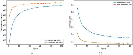
Figure 10. Training and loss metrics: (a) validation performance plot for ResNet50 and model fusion and (b) validation loss plot for ResNet50 and model fusion.

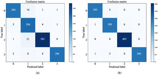
Figure 11. Confusion matrix: (a) ResNet50 confusion matrix and (b) model fusion confusion matrix.

As depicted in Figure 10, the validation accuracy and validation loss trajectories, smoothed exponentially (with a smoothing factor of 5), vividly illustrate the fluctuations in model performance. The improved model outperforms the original model in terms of validation accuracy and validation loss. Specifically, after the residual structure optimization and the integration of the lightweight model EfficientNet-B0, the model’s validation accuracy sees a notable enhancement, while the validation loss experiences a substantial reduction.

From the confusion matrix, it is evident that the fused ResNet50 model demonstrates enhanced performance across all classification tasks. Specifically, the diagonal elements of the confusion matrix have notably increased, indicating a higher number of correctly classified samples. The reduction in values at other positions in the matrix corresponds to fewer misclassifications.

4.1.3. Performance Comparison Between Traditional CNN Architectures with and Without the Optimization Fusion Module

To confirm the broad applicability of the enhanced fusion design, the effectiveness of three well-known neural network models—ResNet50, VGG16, and AlexNet—is evaluated. Under the premise of keeping the model parameter configuration consistent with Section 3.5, the performance indicators before and after adding the optimized fusion structure are tested, respectively. The outcomes of the experiments are presented in Table 6.

Table 6. Validation set performance results for ResNet50, VGG16, AlexNet, and their respective optimized fusion models.

Model	Acc (%)	Pre (%)	Rec (%)	Spe (%)	Kappa (%)	PTT (M)	TTT (H)
ResNet50	95.27	95.40	95.32	98.43	93.66	2.14	3.57
F-ResNet50	98.78	98.82	98.68	99.59	98.36	1.67	2.79
VGG16	93.35	93.18	93.35	97.80	91.09	3.35	5.58
F-VGG16	95.65	95.49	95.51	98.56	94.16	1.83	3.05
AlexNet	88.08	88.21	87.96	95.98	83.99	1.17	1.95
F-AlexNet	89.15	89.20	89.20	96.37	87.46	0.98	1.63

4.1.4. Performance Comparison Between the ECA Module and Other Attention Modules

In this study, the performance of the ECA module is compared with several other popular attention modules to evaluate its effectiveness in brain tumor image classification tasks. The selected comparison modules include the SE attention mechanism and the CBAM attention mechanism. The comparison results are shown in Table 7.

Table 7. Validation set performance results for ECA, SE, and CBAM.

Model	Acc (%)	Pre (%)	Rec (%)	Spe (%)	Kappa (%)
ECA	98.78	98.82	98.68	99.59	98.36
SE	96.16	96.09	96.26	98.72	94.85
CBAM	97.18	97.18	97.15	99.05	96.20

The comparison results shown in Table 7 of this study indicate that the ECA attention mechanism outperforms the SE and CBAM attention mechanisms in brain tumor image classification tasks. The ECA mechanism, with its unique channel attention strategy, can more precisely identify and enhance key features in images, thereby improving the model’s ability to grasp details, more effectively highlighting the lesion areas and increasing classification accuracy. In contrast, although the SE mechanism can weight the channels, its global pooling operation may lose local feature information, resulting in poor performance in identifying complex lesions. The CBAM mechanism, while combining channel and spatial attention, has not achieved the expected results in brain tumor image classification tasks due to its complexity, which may not effectively coordinate the relationships between channel and spatial features, thus affecting overall performance. Therefore, the ECA mechanism outperforms the SE and CBAM mechanisms in key indicators such as accuracy, recall, specificity, and Kappa coefficient, demonstrating its advantages in brain tumor image classification tasks.

4.1.5. p-Value Calculation Result

In the 10 rounds of training conducted on model fusion and ResNet50, the performance deviations of model fusion relative to ResNet50 are calculated after each training round, yielding difference values of −3.51, −2.07, 1.57, −2.56, −2.32, −2.64, −0.53, −2.56, −4.43, and −1.54. The mean of these differences is −2.059, with a standard deviation of 1.647. Based on these data, the t-statistic is further calculated to be −3.953, with a corresponding p-value of 0.0033. This p-value is far below the commonly used significance level of 0.05, indicating that the performance difference between model fusion and ResNet50 is statistically significant, meaning that the performance of model fusion is significantly better than that of ResNet50.

4.1.6. Ablation Experiments

In this part, ablation experiments are conducted to demonstrate the effectiveness of enhancing the residual structure and fusing ResNet50 with the EfficientNetB0 lightweight model. The results of the ablation experiment are shown in Figure 12. Ablation experiments are a systematic approach to evaluate the contribution of each component in a model by progressively removing or modifying them. Figure 13 illustrates how the accuracy of the modified model evolves with the number of training epochs. Table 8 presents the detailed results of these experiments, including visual representations, and outlines the performance metrics. Specifically, after incorporating the ECA attention mechanism and multi-scale convolution, the accuracy (Acc) and Kappa coefficient of the model increased by 1.45% and 1.93%, respectively. After further feature fusion with the EfficientNetB0 lightweight model, the Acc and Kappa coefficients increased by 2.06% and 2.77%, respectively. Regarding the training time, the total training time of the model before fusion is 2.98 h, and after fusion, it decreases to 2.79 h. The outcomes show that the propose enhancements not only significantly improve the model’s performance but also reduce its running time. The ECA attention mechanism enriches the model’s feature representation capabilities and enhances its generalization by incorporating global information. Multi-scale convolution improves the extraction of fine-grained features, enabling the model to handle details with greater precision. Moreover, the use of transfer learning and lightweight models increases training efficiency, minimizes resource usage, and accelerates model training. These enhancements deliver excellent results on the validation data and substantially boost the model’s applicability and practicality in real-world scenarios.

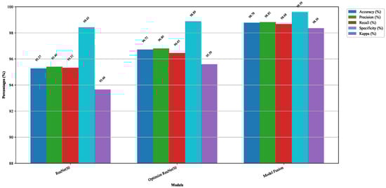
Figure 12. Ablation study results visualized using bar charts.

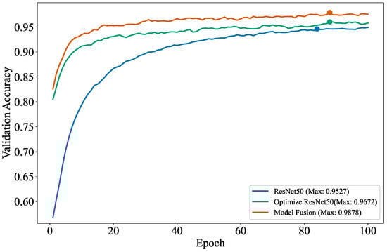
Figure 13. The accuracy and iteration counts from the ablation experiments.

Table 8. Ablation study of optimized fusion of ResNet50 under the validation set.

Model	Acc (%)	Pre (%)	Rec (%)	Spe (%)	Kappa (%)	PTT (M)	TTT (H)
ResNet50	95.27	95.40	95.32	98.43	93.66	2.14	3.57
Optimized ResNet50	96.72	96.80	96.45	98.89	95.59	1.79	2.98
F-ResNet50	98.78	98.82	98.68	99.59	98.36	1.67	2.79

From this figure, the highest validation accuracy of ResNet50 after 100 iterations is 95.27%. Optimized ResNet50 refers to the modification of the residual structure of ResNet50, including the addition of the ECA attention mechanism and multi-scale convolution, and it achieves the highest validation accuracy of 96.72% after 100 epochs. Model fusion refers to the feature fusion of the optimized ResNet50 with the lightweight EfficientNetB0, the highest validation accuracy of model fusion after running 100 rounds is 98.78%.

4.1.7. Visual Analytics

To visually illustrate the impact of model enhancement and fusion, Grad-CAM technology is employed for visual analysis. In the heatmap generated by Grad-CAM, different colors represent the varying degrees of attention the model gives to different areas of the input image. The red areas indicate the parts that the model pays the most attention to; these areas contribute the most to the model’s decision and are typically where the model identifies the most relevant features. The yellow areas indicate a moderate level of attention from the model, contributing to the decision to some extent but not as significantly as the red areas. The blue areas represent the parts with the lowest level of attention, contributing the least to the decision, often consisting of background or unimportant feature areas. Grad-CAM produces heat maps that pinpoint crucial regions in the model’s reasoning process, shedding light on how it reacts to input data. To eliminate interference from redundant black borders, the image is trimmed to remove the surplus areas. As depicted in Figure 14, Column (a) displays the cropped brain tumor images, Column (b) shows the corresponding Grad-CAM visualizations, and Column (c) presents the Grad-CAM images following model optimization and fusion.

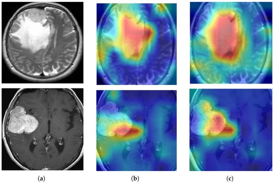
Figure 14. Grad-CAM visualizations: (a) pre-processed brain tumor pictures, (b) Grad-CAM for ResNet50 pictures, and (c) Grad-CAM for the enhanced ResNet50 pictures.

4.1.8. External Dataset Validation

In order to more comprehensively assess the model’s performance and generalization capability, this study introduces the Ultralytics brain tumor dataset for external validation. This dataset contains two categories: negative (images without brain tumors) and positive (images with brain tumors), with the training set consisting of 893 images and the validation set consisting of 223 images. By validating on this independent dataset, the model’s performance can be more objectively evaluated and its stability and accuracy across different data distributions can be ensured. The dataset is shown in Table 9.

Table 9. Ultralytics brain tumor dataset.

Category	Train	Val
Feminine	419	142
Positive	459	81

Validation is conducted on the ResNet50 and Model Fusion models using the Ultralytics brain tumor dataset, and the validation results are shown in Table 10.

Table 10. The validation results of ResNet50 and Model Fusion on the Ultralytics brain tumor dataset.

Model	Acc (%)	Pre (%)	Rec (%)	Spe (%)	Kappa (%)
ResNet50	95.07	96.48	95.80	96.14	89.31
F-ResNet50	97.76	98.59	97.90	98.25	95.14

As can be seen from Table 10, the improved model still shows good improvement effects on external dataset, which fully demonstrates its stronger generalization ability and diagnostic accuracy in brain tumor detection tasks, enabling it to more accurately identify brain tumor images and provide more reliable auxiliary support for clinical diagnosis.

In addition, this study also provides additional validation experiments using the validation datasets provided by the Kaggle platform (https://www.kaggle.com/datasets/tombackert/brain-tumor-mri-data (accessed on 1 November 2024)) and the Hugging Face platform (https://huggingface.co/datasets/Docty/Brain-Tumor-MRI (accessed on 1 November 2024)). Both datasets contain four categories: gliomas, meningiomas, non-tumors, and pituitary tumors, which is consistent with the number of categories in the extended dataset of this article. The weights obtained from training on the expanded dataset in this paper were used to validate the validation set of the additional dataset. The verification results are shown in Table 11 and Table 12 below.

Table 11. The validation results of ResNet50 and Model Fusion on the Kaggle brain tumor dataset.

Model	Acc (%)	Pre (%)	Rec (%)	Spe (%)	Kappa (%)
ResNet50	93.30	94.57	93.78	94.45	91.11
F-ResNet50	96.17	96.88	96.70	97.05	94.23

Table 12. The validation results of ResNet50 and Model Fusion on the Hugging Face brain tumor dataset.

Model	Acc (%)	Pre (%)	Rec (%)	Spe (%)	Kappa (%)
ResNet50	94.55	95.62	94.78	95.53	92.23
F-ResNet50	96.89	97.45	97.33	97.48	94.66

For the validation on the dataset from Kaggle, the accuracy and Kappa value of F-ResNet50 can be improved by 2.87% and 3.12%, respectively, compared to ResNet50. In addition, for Hugging Face dataset, the accuracy and Kappa value of F-ResNet50 improved by 2.34% and 2.43%, respectively. These validation results further confirm the effectiveness of the weights obtained from training on the expanded dataset under different data distributions.

5. Discussions

As can be observed from Table 10, the residual learning mechanism of ResNet50 makes the training and inference process more efficient without losing accuracy. Therefore, this paper chooses ResNet50 as the base model. The significant improvement in validation accuracy and Kappa value of the optimized model, as well as the significant reduction in training time, can be attributed to the following key factors: 1. ECA attention mechanism: By adaptively adjusting the channel weight, the expression of key features is strengthened, and the model’s capacity to identify crucial details is notably enhanced, which in turn boosts classification accuracy. 2. Enhance the residual structure: Substituting the 1 × 1 convolution in the residual structure with multi-scale convolution (encompassing 1 × 1, 3 × 3, and 5 × 5 convolutions) can bolster the model’s proficiency in extracting features across various scales. The 1 × 1 convolution is tasked with fusing channel information, the 3 × 3 convolution is used for local feature extraction, and the 5 × 5 convolution captures broader contextual details. Additionally, the quantity of parameters is diminished through the application of 1 × 1 convolution. 3. Transfer learning: By freezing model parameters and subsequently fine-tuning based on pre-trained models, it significantly reduces training time and computational resource consumption while swiftly adapting to new tasks and enhancing model performance. 4. EfficientNetB0 lightweight model feature fusion: EfficientNet-B0 achieves lightweight through the composite scaling method (expanding depth, width, and resolution simultaneously), and its feature fusion mechanism efficiently integrates multi-scale features, improving model performance while reducing model running time. As shown in Figure 10, thanks to the influence of transfer learning, the improved model exhibited a high initial validation accuracy early in the training phase. This indicates that transfer learning significantly accelerated the model’s convergence speed and endowed it with strong generalization capability right from the start of training. As shown in Figure 11, the confusion matrix indicates that the ResNet50 model, enhanced with the ECA module, multi-scale convolution, and lightweight feature fusion, excels in managing intricate patterns and comprehensive data. It effectively distinguishes between various types of data, significantly enhancing the model’s overall performance.

In Figure 14, Grad-CAM generates a heat map through gradient calculations, using a “jet” color mapping where red, yellow, and blue represent high, medium, and low contribution regions, respectively, highlighting key areas in the image for classification decisions. From the images in Figure 14, it is seen that Figure 14a shows the cropped brain tumor images, which have been preprocessed to remove excess black edges. Figure 14b displays the Grad-CAM visualization results of the ResNet50 model in its original state. It can be seen that the ResNet50 model mainly focuses on the lesion area, indicating that the model is capable of recognizing key areas of the brain tumor. Specifically, the red and yellow areas in the heat map are significantly concentrated in the tumor region, indicating that the model has a high activation intensity in these areas, thus confirming the model’s ability to identify key features of brain tumors. This clustering phenomenon suggests that the model has a high sensitivity for feature extraction of the tumor areas during the inference process, effectively distinguishing tumor regions from non-tumor regions. Figure 14c shows a broader area of attention with increased focus on the lesion area. It is noteworthy that areas that were originally blue (indicating low attention) have transformed into yellow or red in the enhanced model (indicating higher attention), while the originally yellow areas have changed to red, demonstrating a significant increase in the model’s focus on these areas. This transformation indicates that the optimized fusion has enhanced the model’s focusing ability on the affected areas, thus improving the accuracy of brain tumor detection.

This study significantly improves the accuracy and efficiency of brain tumor classification by optimizing the ResNet50 model and combining it with the lightweight EfficientNetB0 model. The optimized ResNet50 model achieves an accuracy of 98.78% on the validation set, which is an improvement of 3.51% over the original model, with a Kappa value increase of 4.7%. Meanwhile, the training efficiency of the model is also significantly enhanced, reducing the training time per epoch from 2.14 min to 1.67 min and the total training time from 3.57 h to 2.79 h. These improvements not only enhance the model’s performance but also increase its feasibility in practical applications. By incorporating the ECA attention mechanism and multi-scale convolutions, the model excels in recognizing key features, particularly when dealing with complex patterns and comprehensive data. Additionally, the lightweight design of EfficientNetB0 reduces the model’s runtime while enhancing performance. These results indicate that the optimized model can diagnose brain tumors earlier and more accurately, thereby improving treatment outcomes and survival rates for patients. However, this study also has some limitations. First, the scale of the experimental data is limited, and the model’s generalization ability on large-scale datasets (on the order of ${10}^4$–${10}^5$) needs further validation. Second, although the ECA attention mechanism demonstrates significant effects in this study, its performance advantages require further confirmation through systematic comparisons with other attention mechanisms (such as CBAM, SE, etc.). Moreover, the model’s performance may vary when dealing with different types of brain tumors, which needs validation on more diverse datasets. In addition, systematic evaluations of its inference speed, memory usage, and computational efficiency on real clinical hardware (such as medical edge devices, embedded systems, or hospital-grade servers) have not yet been conducted. In the future, we will seek cooperation with some hospitals to verify the proposed model in clinical hardwares and further optimize its accuracy. Finally, despite the improved interpretability of the model through Grad-CAM technique, finding better ways to explain the model’s decision-making process remains a challenge in practical applications. Future research will focus on further validating the model’s generalization ability, optimizing the model architecture to enhance its adaptability and feasibility, and exploring the model’s performance across different types of brain tumors, aiming for applications in broader scenarios.

6. Conclusions

This study significantly improved the performance of brain tumor classification by optimizing the ResNet50 model and combining it with the lightweight EfficientNetB0 model. The optimized model exhibited higher classification accuracy on the validation set while greatly reducing training time and increasing training efficiency. These improvements make the model more feasible for practical applications, allowing for earlier and more accurate diagnosis of brain tumors, thereby enhancing patient treatment outcomes and survival rates. Additionally, the introduction of the ECA attention mechanism and multi-scale convolution enhanced the model’s ability to recognize key features. The model particularly showcased outstanding performance in handling complex patterns and comprehensive data. The lightweight design of EfficientNetB0 further enhanced the model’s performance while reducing runtime. These achievements not only improved the model’s performance but also strengthened its adaptability and feasibility in real-world applications, holding significant clinical application value.

References

- Wu, G.; Chen, Y.; Wang, Y.; Yu, J.; Lv, X.; Ju, X.; Shi, Z.; Chen, L.; Chen, Z. Sparse representation-based radiomics for the diagnosis of brain tumors. IEEE Trans. Med. Imaging 2017, 37, 893–905. [Google Scholar] [CrossRef]
- Sahaai, M.B.; Karthika, K.; Theoderaj, A.K.C. EC-HDLNet: Extended coati-based hybrid deep dilated convolutional learning network for brain tumor classification. Biomed. Signal Process. Control 2025, 107, 107865. [Google Scholar] [CrossRef]
- Mallouk, O.; Joudar, N.-E.; Ettaouil, M. ODTL: An Optimal Deep Transfer Learning model for brain tumor classification. Neurocomputing 2025, 649, 130747. [Google Scholar] [CrossRef]
- Hassan, E.; Ghadiri, H. Advancing brain tumor classification: A robust framework using EfficientNetV2 transfer learning and statistical analysis. Comput. Biol. Med. 2024, 185, 109542. [Google Scholar] [CrossRef]
- Sultan, H.; Ullah, N.; Hong, J.S.; Kim, S.G.; Lee, D.C.; Jung, S.Y.; Park, K.R. Estimation of fractal dimension and segmentation of brain tumor with parallel features aggregation network. Fractal Fract. 2024, 8, 357. [Google Scholar] [CrossRef]
- Arnaud, A.; Forbes, F.; Coquery, N.; Collomb, N.; Lemasson, B.; Barbier, E.L. Fully automatic lesion localization and characterization: Application to brain tumors using multiparametric quantitative MRI data. IEEE Trans. Med. Imaging 2018, 37, 1678–1689. [Google Scholar] [CrossRef]
- Huang, Z.; Duan, J.; Xie, Y.; Liu, Y. UDNet: Unified Deep Network based on Transformer and Multi-stage Fusion for brain tumor classification from undersampled MRI. Neurocomputing 2025, 619, 129109. [Google Scholar] [CrossRef]
- Wang, J.; Lu, S.-Y.; Wang, S.-H.; Zhang, Y.-D. RanMerFormer: Randomized vision transformer with token merging for brain tumor classification. Neurocomputing 2024, 573, 127216. [Google Scholar] [CrossRef]
- Hossain, S.; Chakrabarty, A.; Gadekallu, T.R.; Alazab, M.; Piran, M.J. Vision transformers, ensemble model, and transfer learning leveraging explainable AI for brain tumor detection and classification. IEEE J. Biomed. Health Inform. 2023, 28, 1261–1272. [Google Scholar] [CrossRef]
- Disci, R.; Gurcan, F.; Soylu, A. Advanced brain tumor classification in MR images using transfer learning and pre-trained deep CNN models. Cancers 2025, 17, 121. [Google Scholar] [CrossRef]
- Chen, C.; Isa, N.A.M.; Liu, X. A review of convolutional neural network based methods for medical image classification. Comput. Biol. Med. 2025, 185, 109507. [Google Scholar] [CrossRef]
- Sarvamangala, D.R.; Kulkarni, R.V. Convolutional neural networks in medical image understanding: A survey. Evol. Intell. 2022, 15, 1–22. [Google Scholar] [CrossRef]
- Zelik, Y.B.; Altan, A. Overcoming nonlinear dynamics in diabetic retinopathy classification: A robust AI-based model with chaotic swarm intelligence optimization and recurrent long short-term memory. Fractal Fract. 2023, 7, 598. [Google Scholar]
- Abraham, L.A.; Palanisamy, G.; Goutham, V. Dilated convolution and YOLOv8 feature extraction network: An improved method for MRI-based brain tumor detection. IEEE Access 2025, 13, 27238–27256. [Google Scholar] [CrossRef]
- Guder, O.; Cetin-Kaya, Y. Optimized attention-based lightweight CNN using particle swarm optimization for brain tumor classification. Biomed. Signal Process. Control 2025, 100, 107126. [Google Scholar] [CrossRef]
- Agrawal, A.; Chaki, J. CerebralNet meets Explainable AI: Brain tumor detection and classification with probabilistic augmentation and a deep learning approach. Biomed. Signal Process. Control 2025, 110, 108210. [Google Scholar] [CrossRef]
- Gupta, S.C.; Vijayvargiya, S.; Bhattacharjee, V. Role of Feature Diversity in the Performance of Hybrid Models—An Investigation of Brain Tumor Classification from Brain MRI Scans. Diagnostics 2025, 15, 1863. [Google Scholar] [CrossRef]
- Tang, Z.; Xu, Y.; Jin, L.; Aibaidula, A.; Shen, D. Deep Learning of Imaging Phenotype and Genotype for Predicting Overall Survival Time of Glioblastoma Patients. IEEE Trans. Med Imaging 2020, 39, 2100–2109. [Google Scholar] [CrossRef]
- Kumar, S.; Choudhary, S.; Jain, A.; Singh, K.; Ahmadian, A.; Bajuri, M.Y. Brain tumor classification using deep neural network and transfer learning. Brain Topogr. 2023, 36, 305–318. [Google Scholar] [CrossRef]
- Mithun, M.S.; Jawhar, S.J. Detection and classification on MRI images of brain tumor using YOLO NAS deep learning model. J. Radiat. Res. Appl. Sci. 2024, 17, 101113. [Google Scholar] [CrossRef]
- Guo, J.; Xu, P.; Wu, Y.; Tao, Y.; Han, C.; Lin, J.; Zhao, K.; Liu, Z.; Liu, W.; Lu, C. CroMAM: A cross-magnification attention feature fusion model for predicting genetic status and survival of gliomas using histological images. IEEE J. Biomed. Health Inform. 2024, 28, 7345–7356. [Google Scholar] [CrossRef]
- Alzahrani, S.M. ConvAttenMixer: Brain tumor detection and type classification using convolutional mixer with external and self-attention mechanisms. J. King Saud-Univ.-Comput. Inf. Sci. 2023, 35, 101810. [Google Scholar] [CrossRef]
- Li, Z.; Zhou, X. A Global-local parallel dual-branch deep learning model with attention-enhanced feature fusion for brain tumor MRI classification. Comput. Mater. & Contin. 2025, 83, 739. [Google Scholar]
- Janarthan, S.; Thuseethan, S.; Rajasegarar, S.; Lyu, Q.; Zheng, Y.; Yearwood, J. LiRAN: A lightweight residual attention network for in-field plant pest recognition. IEEE Trans. Agrifood Electron. 2025, 3, 167–178. [Google Scholar] [CrossRef]
- Sekhar, A.; Biswas, S.; Hazra, R.; Sunaniya, A.K.; Mukherjee, A.; Yang, L. Brain tumor classification using fine-tuned GoogLeNet features and machine learning algorithms: IoMT enabled CAD system. IEEE J. Biomed. Health Inform. 2021, 26, 983–991. [Google Scholar] [CrossRef]
- Isunuri, B.V.; Kakarla, J. EfficientNet and multi-path convolution with multi-head attention network for brain tumor grade classification. Comput. Electr. Eng. 2023, 108, 108700. [Google Scholar] [CrossRef]
- Alnageeb, M.H.O.; Supriya, M.H. Real-time brain tumour diagnoses using a novel lightweight deep learning model. Comput. Biol. Med. 2025, 192, 110242. [Google Scholar] [CrossRef]
- Shaheema, S.B.; Muppalaneni, N.B. Explainability based Panoptic brain tumor segmentation using a hybrid PA-NET with GCNN-ResNet50. Biomed. Signal Process. Control 2024, 94, 106334. [Google Scholar] [CrossRef]
- Verma, V.; Gupta, D.; Gupta, S.; Uppal, M.; Anand, D.; Ortega-Mansilla, A.; Alharithi, F.S.; Almotiri, J.; Goyal, N. A deep learning-based intelligent garbage detection system using an unmanned aerial vehicle. Symmetry 2022, 14, 960. [Google Scholar] [CrossRef]
- Zhou, T.; Ruan, S.; Hu, H. A literature survey of MR-based brain tumor segmentation with missing modalities. Comput. Med Imaging Graph. 2023, 104, 102167. [Google Scholar] [CrossRef]
- Saifullah, S.; Pranolo, A.; Dreżewski, R. Comparative analysis of image enhancement techniques for brain tumor segmentation: Contrast, histogram, and hybrid approaches. arXiv 2024, arXiv:2404.05341. [Google Scholar] [CrossRef]
- Annadurai, A.; Sureshkumar, V.; Jaganathan, D.; Dhanasekaran, S. Enhancing medical image quality using fractional order denoising integrated with transfer learning. Fractal Fract. 2024, 8, 511. [Google Scholar] [CrossRef]
- Feng, M.; Cai, Y.; Yan, S. Enhanced ResNet50 for diabetic retinopathy classification: External attention and modified residual branch. Mathematics 2025, 13, 1557. [Google Scholar] [CrossRef]
- Liang, H.; Zhou, H.; Zhang, Q.; Wu, T. Object detection algorithm based on context information and self-attention mechanism. Symmetry 2022, 14, 904. [Google Scholar] [CrossRef]
Disclaimer/Publisher’s Note: The statements, opinions and data contained in all publications are solely those of the individual author(s) and contributor(s) and not of MDPI and/or the editor(s). MDPI and/or the editor(s) disclaim responsibility for any injury to people or property resulting from any ideas, methods, instructions or products referred to in the content. |
© 2025 by the authors. Licensee MDPI, Basel, Switzerland. This article is an open access article distributed under the terms and conditions of the Creative Commons Attribution (CC BY) license (https://creativecommons.org/licenses/by/4.0/).