Autonomous Flight in Hover and Near-Hover for Thrust-Controlled Unmanned Airships

Abstract

The ability of airships to fly in hover is a major plus of this category of flying vehicles. However, especially for the case of autonomous flight, this feature can be exploited only recurring to a carefully designed layout of the thrusters on board. Furthermore, the thrusters need to be suitably governed by a dedicated control algorithm. This paper explores a scheme for the control in hover of a thrust-controlled airship without thrust vector control, also assessing its effectiveness in near-hover positioning problems. The control scheme proposed herein extends the capability of a stability augmentation and guidance controller for forward flight, previously introduced by the authors for a conceptually similar airship. A control action based on a system of thrust forces required for hover, and additional thrust components for stabilizing and steering the airship in slow (near-hover) navigation, is thoroughly described. The ensuing control suite is applied and tested in the present paper on the high-fidelity virtual model of a five-thruster airship, showing reasonable stability levels and navigation accuracy of the controlled system.

1. Introduction

Within the growing technical field of lighter-than-air (LTA) flying vehicles, unmanned airships are gaining a special interest for applications in very-low- or very-high-altitude atmospheric missions. Targets of the former include inspection of pipelines or power lines and indoor/quasi-indoor operations like social event photography/video recording [1,2,3]. The latter include high-altitude pseudo-satellite (HAPS) missions, typically carried out in the top layers of the atmosphere (>30 km from ground) [4,5,6,7].

The design requirements associated with such mission profiles are significantly different from one another, yielding generally bigger volumes and technological complexity for high-altitude airships (HAAs) than for low-altitude machines [6,7,8,9,10]. However, in both cases LTAs offer technically advantageous and credible solutions for unmanned flight, merging the superior endurance performance of fixed-wing aircraft to the maneuverability of multi-copters. This effect is especially promising for low-altitude drone applications, considering the major shortcoming of now-widespread battery-fed multi-copters, which feature good maneuvering ability as well as a slow flight/hovering capability which fixed-wing aircraft do not allow, but which invariably suffer from poor endurance—which is even more starkly reduced, compared to airships.

As is known, the comparatively bigger size (e.g., volume, cross and side area) to inertia ratio typical of airships tends to exacerbate stability and controllability issues, compared to other flying machines [11,12,13,14,15], in turn making flight for this class of aircraft potentially much disturbance-prone and poorly accurate, for instance in trajectory-tracking problems [16]. Tackling this issue requires the careful design of automatic flight controllers, which on unmanned airships act towards artificial stabilization and guidance as well. Much literature has been devoted in relatively recent times to the application of diverse control techniques to forward flight and terminal maneuvers of airships featuring aerodynamic control  [17,18,19,20,21] or to the industrially adopted solution of thrust vector control (TVC) [22,23]. Some attention has also been devoted to station keeping tasks in a steady wind condition for a few specific configurations [24,25,26].

Drawing the weight-optimal and simplicity-oriented design philosophy from the field of small multi-copter drones, a careful choice of the configuration of the thrusters on board an airship has been in the focus of recent research by the authors [16,27]. In such a configuration, thrusters are employed for both propulsion and flight control/steering. Correspondingly, movable surfaces are removed in favor of fixed, purely stabilizing empennages.

An advantage of a thrust-based configuration is in its generally lower complexity compared to aerodynamically controlled airships, especially when no thrust vector control (TVC) is considered, thus reducing the number of actuators and related power control components on board. Furthermore, the dual use of thrusters for both propulsion and attitude control/steering should help in reducing the weight of the overall plants on board, required for usual forward flight phases. Finally, the adoption of deflectable control surfaces does not carry any significant advantage in control authority in hovering or at very low airspeed values, where dynamic pressure and aerodynamic forces are minimal.

On the other hand, a suite of thrusters rigidly oriented with respect to the airship (i.e., considering no TVC) needs to be carefully configured, to grant the required control authority. Detailed studies on the topic have been carried out [27], introducing procedures to design purely thrust-controlled airships with no TVC, accounting for performance in forward flight and optimizing control effectiveness vs. control use.

A performance comparison of a thrust-controlled airship vs. a standard, aerodynamically controlled baseline has been presented [16] analyzing fully automated forward flight and non-aggressive navigation maneuvers (e.g., flat turns, climbs and descents) at typical cruising airspeed values, also in the presence of wind disturbances. Coupled with a purpose-designed stability augmentation and guidance system, the thrust-based configuration was shown to display a satisfying performance, generally comparable to or better than a corresponding aerodynamically controlled baseline.

In the present research, the performance of a thrust-controlled airship with no TVC is further assessed, considering the two peculiar flight cases of stationing in hover and near-hover maneuvers. As is known, the dramatically low values of dynamic pressure (which is null in hover) in such flight conditions make an aerodynamically controlled airship generally marginally stable as well as poorly controllable. These features are not typical of a purely thrust-controlled airship, which is also capable of managing equilibrium and steering at very low speed (near-hover) or in hover. On the other hand, also for a thrust-controlled airship, the ineffectiveness of stabilizing empennages and the general modification in the response of the airship in hover with respect to forward flight requires a radical rethinking of the control system structure.

In this research, a force-based control scheme is introduced for the task. The architecture of the controller features two conceptual layers. A first one computes and applies the control solution needed for hover, in terms of thrust from all the thrusters on board. This would be sufficient for keeping the airship in static equilibrium in ideal undisturbed conditions with null dynamic pressure (zero airspeed). The second control layer computes the system of additional thrust contributions to steer the airship, under the hypothesis of negligible dynamic pressure (near-hover). The control action from this layer comes again in the form of additional thrust components from all thrusters, which are conceptually added to the components required for equilibrium in hover (first layer).

The proposed control architecture is model-based, since the thrust components required for either static equilibrium or steering are computed through the closed-form solution of the airship static force and moment balance equations.

In the first section of the paper, the thrust components required for equilibrium in hover and steering in near-hover are thoroughly described and investigated.

Next, control laws binding such force or torque components to feed-back signals are introduced, closing loops with both stabilization and near-hover navigation tasks. In particular, the transition from forward flight to pure hover and a three-dimensional station keeping solution for hover control are presented.

Finally, the performance of the proposed control system is demonstrated in a high-fidelity, fully non-linear virtual environment, showing promising results in the autonomous flight control of a realistic thrust-controlled test-bed.

2. A General Model for Airship Dynamics

As stated in the introduction (Section 1), two logical layers are envisaged in the formulation of control for autonomous flight in hovering and near-hovering conditions. The outcome of both logical layers is a thrust requirement from each thruster on board. In order to compute these thrust requirements, models describing static equilibrium in hover and the reaction of the airship in hover to changes in thrust are required.

Paving the way for introducing such models, a general model for the flight dynamics of an airship considered as a rigid body will be outlined here. The effect of the hypothesis of hovering flight will be shown on this general formulation. This model will be further manipulated in the next sections, as required for the control synthesis tasks of interest in this work.

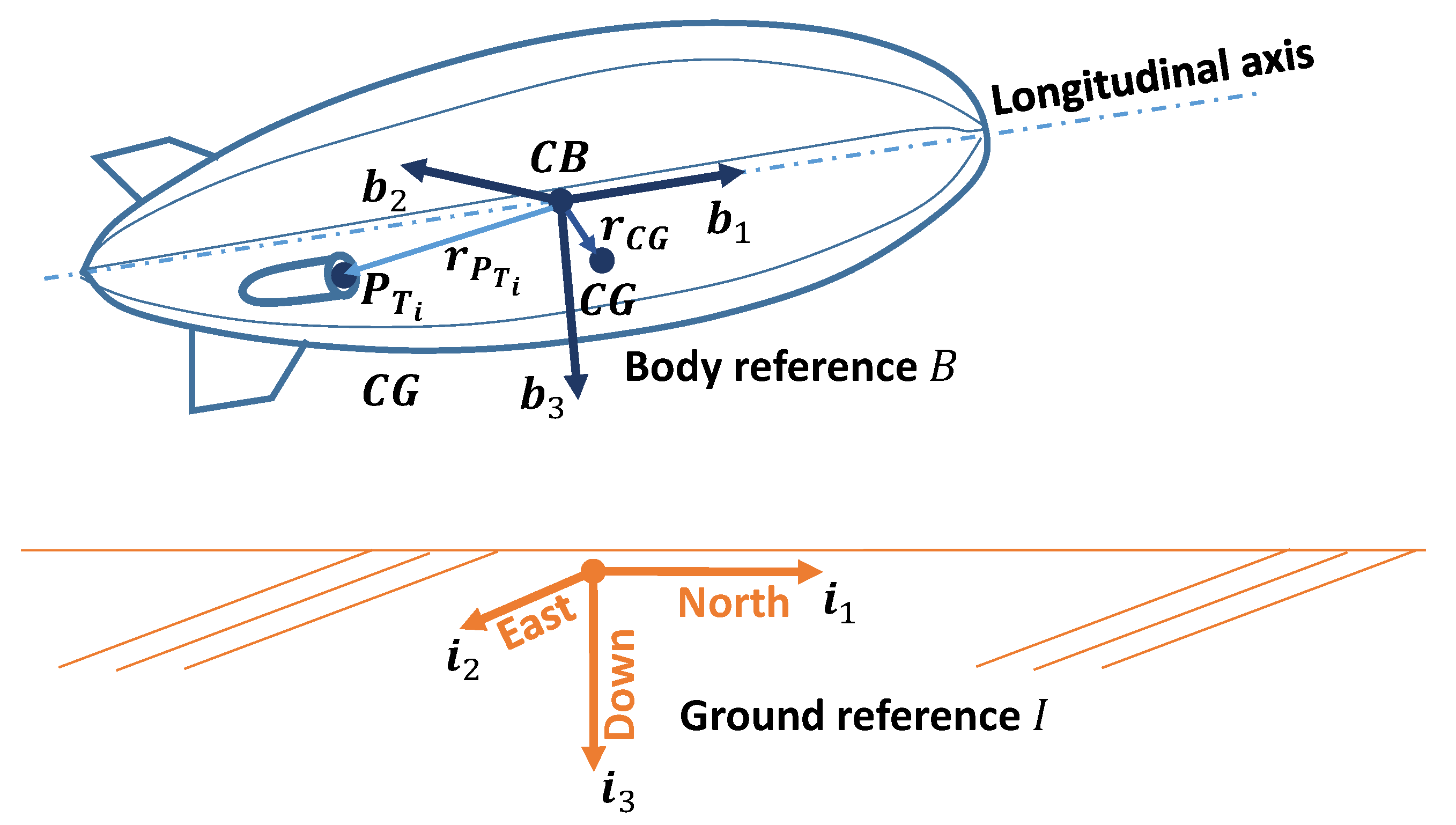
2.1. Airship Flight Dynamics Model: General Formulation

A general model of the dynamics of an airship both in hovering and forward flight in three-dimensional space may be based on the usual balance equations of momentum and moment of momentum. The forcing terms on the right hand side (r.h.s.) of both balance equations will be due to aerodynamics, buoyancy, gravity and thrust.

Referring to Figure 1, considering the airship as a rigid body and taking as a reference point for moment of momentum balance the center of buoyancy $\mathit{CB}$ of the airship, as is customary in the literature on airship dynamics [11,12,27], it is possible to write the balance equations in vector form as follows,

$${\mathit{M}}_{\mathit{CB}}{\dot{\mathit{w}}}_{\mathit{CB}}+{\mathit{w}}_{{\mathit{CB}}_{\backslash \swarrow }}{\mathit{M}}_{\mathit{CB}}{\mathit{w}}_{\mathit{CB}}={\mathit{s}}_{\mathit{CB}}.$$

(1)

On the left hand side (l.h.s.) of Equation (1), the generalized velocity ${\mathit{w}}_{\mathit{CB}}$ is a six-dimensional vector, analytically defined as

$${\mathit{w}}_{\mathit{CB}}={\left\{{\mathit{v}}_{\mathit{CB}},{\mathit{\omega }}_{\mathcal{B}/\mathcal{I}}\right\}}^T,$$

(2)

thus wrapping together the velocity of the $\mathit{CB}$, i.e., ${\mathit{v}}_{\mathit{CB}}$, and the rotational rate ${\mathit{\omega }}_{\mathcal{B}/\mathcal{I}}$ of the airship body reference $\mathcal{B}$ with respect to the ground inertial reference $\mathcal{I}$. On the same l.h.s. of Equation (1), the generalized mass ${\mathit{M}}_{\mathit{CB}}$ of the system is a six-dimensional tensor constituted as

$${\mathit{M}}_{\mathit{CB}}=\left[\begin{array}{cc}m\mathit{I}& {\mathit{S}}_{\mathit{CB}}^T\\ {\mathit{S}}_{\mathit{CB}}& {\mathit{J}}_{\mathit{CB}}\end{array}\right],$$

(3)

where m is the mass of the airship, $\mathit{I}$ represents a three-dimensional identity, and ${\mathit{S}}_{\mathit{CB}}$ and ${\mathit{J}}_{\mathit{CB}}$ are the static moment and moment of inertia of the airship from $\mathit{CB}$, respectively.

The generalized forcing term ${\mathit{s}}_{\mathit{CB}}$ on the r.h.s. of Equation (1) can be split in the four aforementioned contributions due to aerodynamics, buoyancy, gravity and thrust, in this order on the r.h.s. of Equation (4),

$${\mathit{s}}_{\mathit{CB}}={\mathit{s}}_{\mathit{CB}}^a+{\mathit{s}}_{\mathit{CB}}^b+{\mathit{s}}_{\mathit{CB}}^g+{\mathit{s}}_{\mathit{CB}}^t.$$

(4)

In Equation (4), each component ${\mathit{s}}_{\mathit{CB}}^{(·)}$ is a six-dimensional term composed of a force ${\mathit{f}}^{\left(·\right)}$ and moment $m_{\mathit{CB}}^{\left(·\right)}$ with respect to the center of buoyancy $\mathit{CB}$, yielding

$${\mathit{s}}_{\mathit{CB}}^{\left(·\right)}={\left\{{\mathit{f}}^{\left(·\right)},{\mathit{m}}_{\mathit{CB}}^{\left(·\right)}\right\}}^T.$$

(5)

2.2. Representation of the Equations of Motion in Body Components

A representation of all terms in Equations (2)–(4) allows Equation (1) to be made explicit, thus in particular allowing it to be practically integrated in time.

With this aim, all terms are expressed by components in the airship body frame $\mathcal{B}$ as typical to aircraft dynamics [28]. In particular, the generalized velocity vector takes the form ${\mathit{w}}_{\mathit{CB}}^{\mathcal{B}}={\left\{U,V,W,p,q,r\right\}}^T$, where the first three are the usual components of velocity and the last three of rotational speed. Superscript ${(·)}^{\mathcal{B}}$ means a representation by components in the body frame $\mathcal{B}$.

Through passages well documented in the literature for the case of airships [11,12,16,27], adopting the $\mathit{CB}$ as the origin of the body frame, expressions for the forcing terms can be obtained. Only major results of use for the discussion to follow will be recalled herein.

2.2.1. Aerodynamic Active and Reaction Terms

For aerodynamics (i.e., term ${\mathit{s}}_{\mathit{CB}}^a$), it is worth recalling that for the case of airships typically two terms exist, namely an active term ${\mathit{s}}_{\mathit{CB}}^{a,b}$ and a reaction term ${\mathit{s}}_{\mathit{CB}}^{a,m}$.

The active term models the action exerted by the air pressure field on the wet surface of the airship (including envelope and fins), in a similar fashion to aircraft. In body components, this term is typically expressed as a function of dynamic pressure (which in still air can be measured based on the velocity of the airship as $\frac{1}{2}\rho {\left|{\mathit{v}}_{\mathit{CB}}\right|}^2$, wherein $\rho$ is the density of air), a reference surface (which is taken as the cubic root of the volume of the airship envelope squared, i.e., $Vo{l}^{\frac{2}{3}}$), and a six-dimensional array of force and moment coefficients ${\mathit{c}}_{\mathit{CB}}^{\mathcal{B}}$. The resulting expression yields

$${\mathit{s}}_{\mathit{CB}}^{{a,b}^{\mathcal{B}}}=\frac{1}{2}\rho {\left|{\mathit{v}}_{\mathit{CB}}\right|}^{2}Vo{l}^{\frac{2}{3}}{\mathit{c}}_{\mathit{CB}}^{\mathcal{B}}.$$

(6)

The coefficients of aerodynamic force and moment in the array ${\mathit{c}}_{\mathit{CB}}^{\mathcal{B}}$ on airships of standard back-tailed configuration are typically functions of the current value of the generalized velocity ${\mathit{w}}_{\mathit{CB}}^{\mathcal{B}}$, and of control variables measuring the deflection of control surfaces on the tail. The latter are wrapped in ${\mathit{u}}^a={\left\{{\delta }_e,{\delta }_a,{\delta }_r\right\}}^T$, i.e., elevator, aileron and rudder controls, respectively. These dependencies yield the implicit functional form ${\mathit{c}}_{\mathit{CB}}^{\mathcal{B}}={\mathit{c}}_{\mathit{CB}}^{\mathcal{B}}\left({\mathit{w}}_{\mathit{CB}}^{\mathcal{B}},{\mathit{u}}^a\right)$.

The reaction aerodynamic term ${\mathit{s}}_{\mathit{CB}}^{a,m}$, often called apparent mass term [10,12], is associated with the inertia of the air surrounding the airship envelope, which is displaced in case of a maneuver of the latter. In principle, this forcing term shows up whenever a solid accelerates in a fluid. However, its intensity is proportional to the displaced fluid mass and therefore totally negligible compared to other forces for winged aircraft traveling in air, given their inertia and volume. For airships instead, this term should be accounted for, since the overall mass of the airship is not excessively far from that of the displaced air, due to its sizeable volume and limited inertia. Irrespective of the representation (in body frame, ground frame, etc.) this term is related to linear and rotational acceleration, yielding ${\mathit{s}}_{\mathit{CB}}^{a,m}={\mathit{s}}_{\mathit{CB}}^{a,m}\left({\dot{\mathit{w}}}_{\mathit{CB}}\right)$.

Considering the two aerodynamic terms, it is worth noting that their mutual balance may be typically different depending on the flight condition. In particular, the active term reduces proportionately to the square of the airspeed when decelerating from forward flight to hover, then it is typically negligible near hover and identically null in hover. Conversely, the reaction term is not bound to velocity (i.e., to airspeed in still air) but to acceleration, therefore it may be either null or not both in forward flight and hover. For instance, a steady (trimmed) forward flight condition will be associated with a null aerodynamic reaction term, whereas a fixed-point rotational acceleration around the $\mathit{CB}$ will produce a non-null value of this forcing term.

A further remark on the aerodynamic term concerns the loss of authority of fins when the dynamic pressure is reduced. As seen, ${\mathit{s}}_{\mathit{CB}}^{a,b}$ is a function of ${\mathit{u}}^a$ through the coefficients ${\mathit{c}}_{\mathit{CB}}$. This dependence represents the ability of deflectable surfaces to influence the aerodynamic force and moment exerted on the airship. However, both the fixed stabilization part and the movable control components of the empennages will be generally less effective as the airship reduces its airspeed from forward flight to hover, since the actual intensity of the forcing term is modulated by the dynamic pressure (Equation (6)). In particular, the authority of fins in terms of stability and controllability will be negligible in near-hover, and null in hovering flight. In this respect, the adoption of an alternative way of controlling the airship, not bound to aerodynamic action, is needed in these specific flight conditions. A thrust-based control will be proposed with this aim in the next sections of this paper.

2.2.2. Buoyancy and Gravity

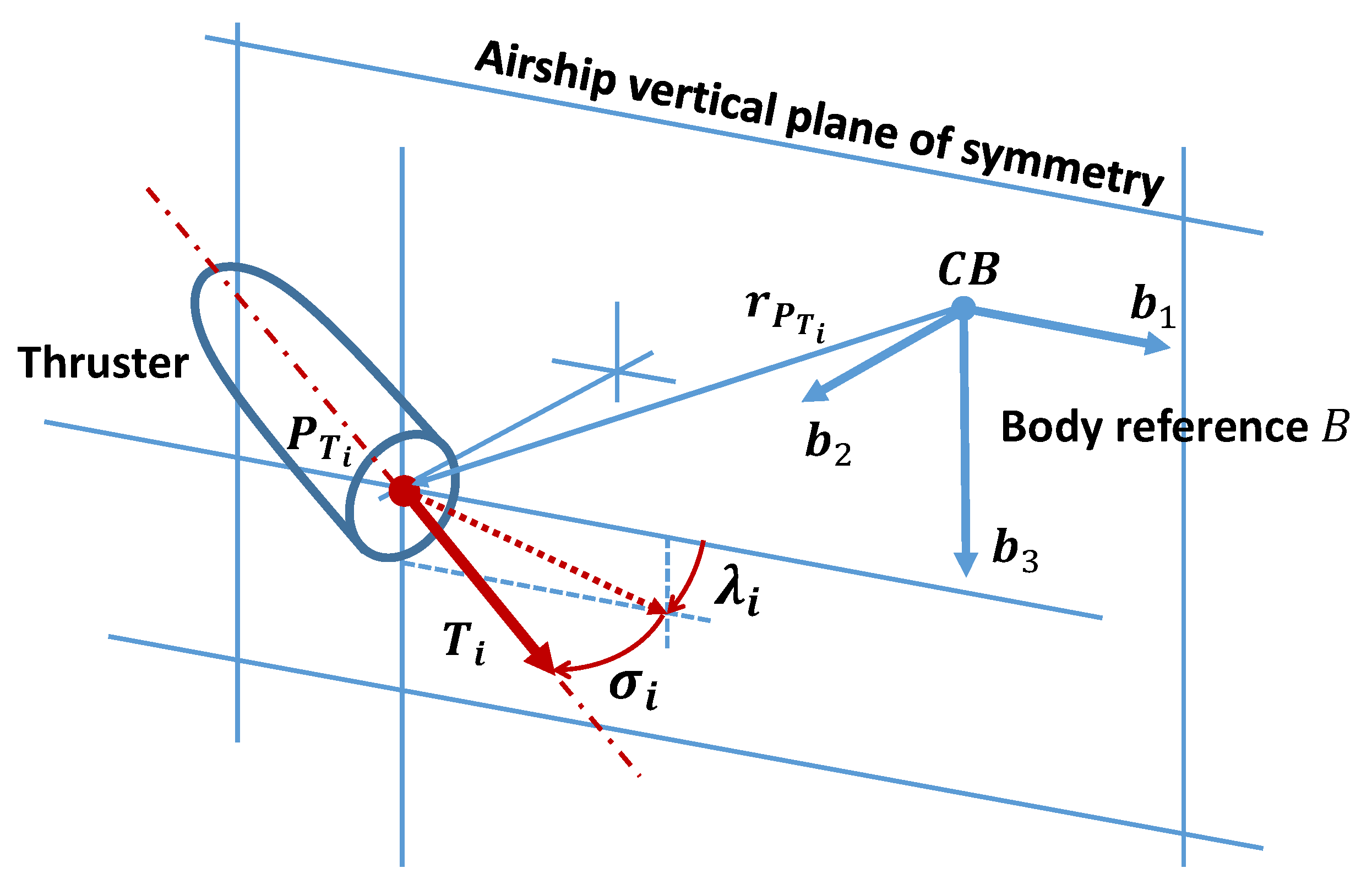
The terms of buoyancy ${\mathit{s}}_{\mathit{CB}}^b$ and gravity ${\mathit{s}}_{\mathit{CB}}^g$ can be easily represented with respect to a ground inertial frame $\mathcal{I}$, where the corresponding forces are aligned with an axis normal to the horizontal plane (i.e., ${\mathit{i}}_3$ in Figure 1), and the ensuing moment is due to the arm of the forces with respect to the measuring point. In particular, since the latter is the center of buoyancy $\mathit{CB}$ in this paper, the moment of buoyancy is identically null by definition.

In order to take the straightforward expressions of these two forcing terms obtained in the ground reference $\mathcal{I}$ to the corresponding expressions in body reference $\mathcal{B}$, the attitude of the body reference frame with respect to the ground one is needed. This can be defined through the three rotation parameters [27,28] measuring roll ($\phi$), pitch ($\vartheta$) and yaw ($\psi$), wrapped together in the array ${\mathit{e}}_{321}^{\mathcal{B}}={\left\{\phi ,\vartheta ,\psi \right\}}^T$.

Correspondingly, implicit functional expressions for both buoyancy and gravity generalized forcing terms in a body reference can be given as ${\mathit{s}}_{\mathit{CB}}^{b,\mathcal{B}}={\mathit{s}}_{\mathit{CB}}^{b,\mathcal{B}}\left(Vol,\rho ,{\mathit{e}}_{321}\right)$ and ${\mathit{s}}_{\mathit{CB}}^{g,\mathcal{B}}={\mathit{s}}_{\mathit{CB}}^{g,\mathcal{B}}\left(m,{\mathit{e}}_{321},{\mathit{r}}_{\mathit{CG}}^{\mathcal{B}}\right)$. In particular, ${\mathit{r}}_{\mathit{CG}}^{\mathcal{B}}$ represents the position of the center of gravity $\mathit{CG}$ of the airship from the center of buoyancy $\mathit{CB}$ (see Figure 1), expressed in body components. Clearly, for assigned and constant mass and geometrical parameters, these forms turn respectively into ${\mathit{s}}_{\mathit{CB}}^{b,\mathcal{B}}={\mathit{s}}_{\mathit{CB}}^{b,\mathcal{B}}\left({\mathit{e}}_{321}\right)$ and ${\mathit{s}}_{\mathit{CB}}^{g,\mathcal{B}}={\mathit{s}}_{\mathit{CB}}^{g,\mathcal{B}}\left({\mathit{e}}_{321}\right)$.

2.2.3. Thrust

The thrust forcing term ${\mathit{s}}_{\mathit{CB}}^t$ is obtained from vectorially composing the contributions from all thrusters on board. For the generic i-th thruster attached to the airship, the corresponding thrust force ${\mathit{T}}_i$ can be modeled as a vector pointing along the longitudinal axis of the thruster, with an intensity $T_i$ given as

$$T_i={\tilde{T}}_i{\tilde{K}}_i\left({\delta }_{T_i}\right){\delta }_{T_i}.$$

(7)

In Equation (7), ${\tilde{T}}_i$ is the nominal value of thrust from the i-th thruster. The control ${\delta }_{T_i}$ modulates the nominal value through the shape function ${\tilde{K}}_i\left({\delta }_{T_i}\right)$. The latter allows the reproduction of possible regime-dependent efficiency effects or non-linear features related to the specific thruster technology. Furthermore, according to the technology implemented in the thruster, a different range of ${\delta }_{T_i}$ values can be considered. In particular, for a piston engine, this control would be limited to a positive value, whereas for electric motors it may be also negative, thus producing an inversion of the thrust force, exploiting a well-known advantage of these types of thrusters with respect to more standard piston-powered ones.

The point of application of the i-th thrust force is point ${\mathit{P}}_{{\mathit{T}}_i}$. Its distance with respect to the $\mathit{CB}$ is defined through the position vector ${\mathit{r}}_{{\mathit{P}}_{{\mathit{T}}_i}}$ (Figure 1 and Figure 2).

The orientation of the i-th thrust vector ${\mathit{T}}_i$ with respect to the airship body reference can be assigned recurring to two angles, namely an angle ${\sigma }_i$ representing the misalignment between the vertical plane of symmetry of the airship (i.e., the plane normal to ${\mathit{b}}_2$ in Figure 1) and the thrust line of the i-th thruster (taken positive to the right of the airship), and angle ${\lambda }_i$, defined between the projection of the i-th thrust line on the vertical plane of symmetry and the longitudinal body axis (positive downwards), as accurately described in [27] and shown in Figure 2.

It should be pointed out that, in case no thrust vector control (TVC) is considered, the thrust settings ${\delta }_{T_i}$ pertaining to all thrusters constitute the array of thrust control inputs available for controlling the airship. This array is here defined as ${\mathit{u}}^t={\left\{{\delta }_1,\dots ,{\delta }_{N_t}\right\}}^T$, where $N_t$ represents the number of thrusters on board. Instead, in case thrust vectoring was of interest, ${\lambda }_i$ and ${\sigma }_i$ would also be included in ${\mathit{u}}^t$. The latter is not the case in this paper, as explained in Section 1.

Employing the definitions in this paragraph, it is possible to assign the total thrust forcing term in body components through the implicit functional form ${\mathit{s}}_{\mathit{CB}}^{t,\mathcal{B}}={\mathit{s}}_{\mathit{CB}}^{t,\mathcal{B}}\left({\mathit{u}}^t,{\sigma }_i,{\lambda }_i,{\mathit{r}}_{{\mathit{P}}_{{\mathit{T}}_i}}^{\mathcal{B}}\right)$. For an assigned and constant placement of the thrusters, in terms of both position and attitude, the latter form is turned into ${\mathit{s}}_{\mathit{CB}}^{t,\mathcal{B}}={\mathit{s}}_{\mathit{CB}}^{t,\mathcal{B}}\left({\mathit{u}}^t\right)$.

3. Control Layers: Thrust for Hover Equilibrium and Near-Hover Steering

In this section, the general model introduced in Section 2 is employed to set up the closed-form computation of the thrust required for static equilibrium (i.e., in hovering flight) and of that needed for steering the airship in near-hover, i.e., close to a hovering condition.

3.1. Control Solution for Static Equilibrium in Hovering Flight for a Thrust-Controlled Airship

As pointed out in Section 2.2.1, in hovering flight ${\mathit{w}}_{\mathit{CB}}=\mathbf{0}$; therefore, the active aerodynamic term can be considered null, ${\mathit{s}}_{\mathit{CB}}^{a,b}=\mathbf{0}$. Provided a model was available for expressing the aerodynamic reaction term ${\mathit{s}}_{\mathit{CB}}^{a,m}$ as an explicit function of ${\dot{\mathit{w}}}_{\mathit{CB}}$, it would be possible to link this term to ${\dot{\mathit{w}}}_{\mathit{CB}}$ appearing on the l.h.s. of the dynamic equation Equation (1), leaving only gravity, buoyancy and thrust as forcing terms on the r.h.s. of dynamic equilibrium [12,27]. Such a model is available for instance through Munk–Jones–DeLaurier theory [29,30,31,32]. Furthermore, in hover accelerations are also null, ${\dot{\mathit{w}}}_{\mathit{CB}}=0$. Therefore, in that case ${\mathit{s}}_{\mathit{CB}}^{a,m}=\mathbf{0}$.

Similarly, in case of a near-hovering condition at very low airspeed, the term ${\mathit{s}}_{\mathit{CB}}^{a,b}\approx \mathbf{0}$ and approximately also ${\mathit{s}}_{\mathit{CB}}^{a,m}$ can be considered negligible if no significant accelerations are experienced by the airship. Therefore, the model shown next for equilibrium in hover can be applied by extension to near-hover as well.

Now, considering the hypotheses on static equilibrium just introduced, for hover (often referred to as a trimmed condition in hovering flight), equilibrium equations can be written in body components in implicit form as

$${\mathit{s}}_{\mathit{CB}}^{b,\mathcal{B}}+{\mathit{s}}_{\mathit{CB}}^{g,\mathcal{B}}+{\mathit{s}}_{\mathit{CB}}^{t,\mathcal{B}}=\mathbf{0}.$$

(8)

To investigate a possible solution of Equation (8), for the case of null roll (${\phi }_0=$ 0) and for a longitudinally symmetric airship, its expression can be rewritten explicitly in body components as follows,

$$\left\{\begin{array}{cccc}\hfill (m-\rho Vol)gsin{\vartheta }_0& =\sum _{i=1}^{N_t}{T}_{i_x},\hfill & \hfill & \mathrm{longitudinal}\mathrm{force}\mathrm{eql}.\hfill \\ \hfill 0& =\sum _{i=1}^{N_t}{T}_{i_y},\hfill & \hfill & \mathrm{lateral}\mathrm{force}\mathrm{eql}.\hfill \\ \hfill -(m-\rho Vol)gcos{\vartheta }_0& =\sum _{i=1}^{N_t}{T}_{i_z},\hfill & \hfill & \mathrm{vertical}\mathrm{force}\mathrm{eql}.\hfill \\ \hfill 0& =\sum _{i=1}^{N_t}\left(T_{i_z}{r}_{{\mathit{P}}_{{\mathit{T}}_{i_y}}}-T_{i_y}{r}_{{\mathit{P}}_{{\mathit{T}}_{i_z}}}\right),\hfill & \hfill & \mathrm{rolling}\mathrm{moment}\mathrm{eql}.\hfill \\ \hfill mg\left(r_{{\mathit{CG}}_z}sin{\vartheta }_0+r_{{\mathit{CG}}_x}cos{\vartheta }_0\right)& =\sum _{i=1}^{N_t}\left(T_{i_x}{r}_{{\mathit{P}}_{{\mathit{T}}_{i_z}}}-T_{i_z}{r}_{{\mathit{P}}_{{\mathit{T}}_{i_x}}}\right),\hfill & \hfill & \mathrm{pitching}\mathrm{moment}\mathrm{eql}.\hfill \\ \hfill 0& =\sum _{i=1}^{N_t}\left(T_{i_y}{r}_{{\mathit{P}}_{{\mathit{T}}_{i_x}}}-T_{i_x}{r}_{{\mathit{P}}_{{\mathit{T}}_{i_y}}}\right),\hfill & \hfill & \mathrm{yawing}\mathrm{moment}\mathrm{eql}.\hfill \end{array}\right.$$

(9)

In Equation (9) subscripts ${(·)}_x$, ${(·)}_y$ and ${(·)}_z$ refer to the first, second and third components in the body frame, respectively. The value ${\vartheta }_0$ represents a reference value for the pitch angle assigned for the hovering condition (i.e., a deck angle in trim).

Assigning the l.h.s. of the system requires defining the mass m, volume $Vol$ and position ${\mathit{r}}_{\mathit{CG}}$ of $\mathit{CG}$ with respect to the $\mathit{CB}$, and ${\vartheta }_0$. Furthermore, when the position of the thrusters is known as well (i.e., positions ${\mathit{r}}_{{\mathit{P}}_{{\mathit{T}}_{\mathit{i}}}}$ are assigned), the only unknowns in Equation (9) are the components of thrust $T_{i_x}$, $T_{i_y}$ and $T_{i_z}$ for the $N_t$ thrusters on board. However, clearly the components of thrust from a same thruster are related to each other by constitution, according to the definition of $T_i$, ${\lambda }_i$ and ${\sigma }_i$ introduced in Section 2.2.3. In particular, by inspection of Figure 2, the following definitions can be retrieved,

$$\left\{\begin{array}{cc}\hfill T_{i_x}& =T_{i}cos{\sigma }_{i}cos{\lambda }_i,\hfill \\ \hfill T_{i_y}& =T_{i}sin{\sigma }_i,\hfill \\ \hfill T_{i_z}& =T_{i}cos{\sigma }_{i}sin{\lambda }_i.\hfill \end{array}\right.$$

(10)

As previously pointed out, if no thrust vector control (TVC) is assumed, then ${\sigma }_i$ and ${\lambda }_i$ are assigned constant values, defining the attitude of a thruster with respect to the airship envelope. In that case, the systems in Equations (9) and (10) considered together produce in general a set of $6+3N_t$ scalar linear constraining relationships, in the $4N_t$ unknowns $T_{i_x}$, $T_{i_y}$, $T_{i_z}$ and $T_i$ for $i=1,\dots ,N_t$.

Now, a solution of the system obtained composing Equations (9) and (10) would produce a set of thrust force values such as to grant equilibrium in hover, thus defining the control action from the first control layer, introduced conceptually in Section 1.

By inspecting the two systems, it can be observed that a solution cannot be universally granted, but its existence depends on the actual number of thrusters on board ($N_t$), their positioning ${\mathit{P}}_{{\mathit{T}}_i}$ and their orientation (${\lambda }_i$, ${\sigma }_i$) within the assumed propulsive configuration of the airship. In practical terms, this result describes the fact that a generic choice of the geometrical placement and orientation of the thrusters on board may result in a propulsive configuration incompatible with static equilibrium in hover.

Conversely, in case the number, positioning and orientation of the thrusters bore a well-posed linear system from Equations (9) and (10), then it could be solved in closed form, in terms of the unknowns $T_{i_x}$, $T_{i_y}$, $T_{i_z}$ and $T_i$, for $i=1,\dots ,N_t$. In particular, in that case, the solution of the system will provide the control values of thrust force, here defined as $T_i=T_i^{\mathrm{hov}}$, needed from each of the $N_t$ thrusters on board for granting static equilibrium in hover.

A closed-form explicit solution can be managed by an onboard controller and is therefore of special interest in practice. The solution would depend on a set of constant data, namely

• Thrusters: the body coordinates ${\mathit{r}}_{{\mathit{P}}_{{\mathit{T}}_i}}^{\mathcal{B}}$ of the thrusters wrt. the center of buoyancy $\mathit{CB}$, and the attitude angles ${\sigma }_i$ and ${\lambda }_i$ of the thrusters with respect to the airship;
• Inertia: the mass m of the system and the body coordinates ${\mathit{r}}_{\mathit{CG}}^{\mathcal{B}}$ of the center of gravity wrt. the center of buoyancy $\mathit{CB}$;
• Buoyancy: the volume $Vol$ of the envelope and the density of air $\rho$ at hovering altitude;
• The assigned pitch angle of the deck in hover ${\vartheta }_0$.

In practice, such data should be assigned as parameters to the controller, for actually carrying out the online computation of the control solution for static equilibrium.

Furthermore, the equilibrium solution in terms of thrust intensity $T_i^{\mathrm{hov}}$ can be converted into a specific thrust setting ${\delta }_{t_i}$ for the corresponding thruster, provided the characteristic of the thruster is assigned.

Later in this paper (Section 5), a case study will be introduced, showing and discussing the specific results obtained from this formulation of equilibrium in hover (Equations (9) and (10)) in a realistic example.

3.2. Control Solution for Airship Steering in Hover and Near-Hover

As shown in Section 3.1, a value of thrust for equilibrium in hover can be obtained in closed form for a suitably arranged layout of the thrusters. However, for stabilizing as well as steering the airship in order to navigate in near-hover conditions, and keep it close to an assigned stationing point without diverging in presence of a disturbance, it is also useful to obtain further control actions from the thrusters. With this aim, considering the airship in equilibrium in hover, it is interesting to investigate a way to obtain an equivalent target system of forces and moments around the $\mathit{CB}$, from the contributions of each thruster on board. This is the second control layer conceptually introduced in Section 1.

In analytic terms, considering the need to position the airship in hover at a target point in three-dimensional space with respect to the ground reference $\mathcal{I}$, it is useful to compute control force components in this frame. These may be employed by a controller to take the airship through a slow near-hover motion to the target position in three-dimensional space, and to keep it there once in place, in the presence of disturbance. Hypothesizing a zero-roll hovering condition (${\phi }_0=$ 0) as in Section 3.1, three control force components are here defined, namely a horizontal force component in the longitudinal body plane $\Delta F_{HF}$ ($HF$ for horizontal-forward), a horizontal force component normal to the longitudinal body plane $\Delta F_{HL}$ ($HL$ for horizontal-lateral) and a vertical force component $\Delta F_V$, i.e., normal to the horizon. These definitions are pictorially explained in the left plot of Figure 3.

Considering moment around $\mathit{CB}$, we introduce three target components. In accordance with the controller architecture envisaged in this paper and described later in Section 4, it is convenient to define the first two components around the body roll and pitch axes, namely $\Delta M_x$ and $\Delta M_y$, whereas the last is a moment component $\Delta M_V$ contained in the horizontal plane, i.e., represented by a vector normal to that plane (see the right plot on Figure 3).

Given these definitions, obtaining an expression of each of the target components from an action of the thrusters on board is possible according to the following set of linear equivalences,

$$\left\{\begin{array}{cccc}\hfill \Delta F_{HF}& =\sum _{i=1}^{N_t}\left(\Delta T_{i_x}cos\vartheta +\Delta T_{i_z}sin\vartheta \right)\hfill & \hfill & \mathrm{horizontal}-\mathrm{forward}\mathrm{force}\mathrm{comp}.\hfill \\ \hfill \Delta F_{HL}& =\sum _{i=1}^{N_t}\left(\Delta T_{i_y}\right)\hfill & \hfill & \mathrm{horizontal}-\mathrm{lateral}\mathrm{force}\mathrm{comp}.\hfill \\ \hfill \Delta F_V& =\sum _{i=1}^{N_t}\left(-\Delta T_{i_x}sin\vartheta +\Delta T_{i_z}cos\vartheta \right)\hfill & \hfill & \mathrm{vertical}\mathrm{force}\mathrm{comp}.\hfill \\ \hfill \Delta M_x& =\sum _{i=1}^{N_t}\left(\Delta T_{i_z}{r}_{{\mathit{P}}_{{\mathit{T}}_{i_y}}}-\Delta T_{i_y}{r}_{{\mathit{P}}_{{\mathit{T}}_{i_z}}}\right),\hfill & \hfill & \mathrm{rolling}\mathrm{moment}\mathrm{comp}.\hfill \\ \hfill \Delta M_y& =\sum _{i=1}^{N_t}\left(\Delta T_{i_x}{r}_{{\mathit{P}}_{{\mathit{T}}_{i_z}}}-\Delta T_{i_z}{r}_{{\mathit{P}}_{{\mathit{T}}_{i_x}}}\right),\hfill & \hfill & \mathrm{pitching}\mathrm{moment}\mathrm{comp}.\hfill \\ \hfill \Delta M_V& =\sum _{i=1}^{N_t}\left(\Delta T_{i_y}{r}_{{\mathit{P}}_{{\mathit{T}}_{i_x}}}-\left(\Delta T_{i_x}cos\vartheta +\Delta T_{i_z}sin\vartheta \right)r_{{\mathit{P}}_{{\mathit{T}}_{i_y}}}\right),\hfill & \hfill & \mathrm{moment}\mathrm{in}\mathrm{horizontal}\mathrm{plane}\mathrm{comp}.\hfill \end{array}\right.$$

(11)

As stated, the l.h.s. of the expressions in Equation (11) represent a set of assigned control force and control moment components. In the next section, the values of these control components will be set through control laws for near-hovering and hovering flight, in closed loop with respect to a suitable set of feed-back variables.

As observed in Section 3.1 for equilibrium in hover, the system in Equation (11) is complemented by the three definitions in Equation (10) (which hold also when substituting symbol $T_i$ with $\Delta T_i$ everywhere in the latter). The resulting linear system of equations may be solved in principle in $\Delta T_{i_x}$, $\Delta T_{i_y}$, $\Delta T_{i_z}$ and $\Delta T_i$, for $i=1,\dots ,N_t$, thus providing a set of thrust components from each thruster equivalent to the force and moment components needed for control.

However, the same comments raised in Section 3.1 concerning the existence of the solution to the systems in Equations (9) and (10) apply also here. A preliminary consistent choice of the configuration of the thrusters on board is required at a design level, to grant the existence of a solution for an assigned set of control force and moment components. Provided the thruster configuration is compatible with the task, the linear system composed of Equations (10) and (11) will be mathematically well-posed and it will be possible to solve it in closed form, yielding an effective way for a controller to compute control components in hover and near-hover.

A remark concerns the generic value of $\vartheta$ in Equation (11), written instead of ${\vartheta }_0$. This is to stress the fact that the system in Equation (11) applies accurately in hovering flight but it can be employed approximately for near-hover, i.e., when the aerodynamic action can be neglected although not null, for computing the thrust contributions needed to obtain a control action defined by the values on the l.h.s. This is relevant in particular when $\vartheta$ is not the desired deck angle for hovering trim but the current—possibly perturbed—value instead.

Notably, only the positions of the thrusters on board ${\mathit{r}}_{{\mathit{P}}_{{\mathit{T}}_i}}^{\mathcal{B}}$, and the attitude angles ${\sigma }_i$ and ${\lambda }_i$ are required as parameters for computing the thrust components corresponding to a desired system of control forces and moments.

The so-obtained values of $\Delta T_i$ can be composed with the reference thrust values $T_i^{\mathrm{hov}}$ and the results converted through the thrusters’ characteristics into thrust settings ${\delta }_{T_i}$ demanded from the actuators.

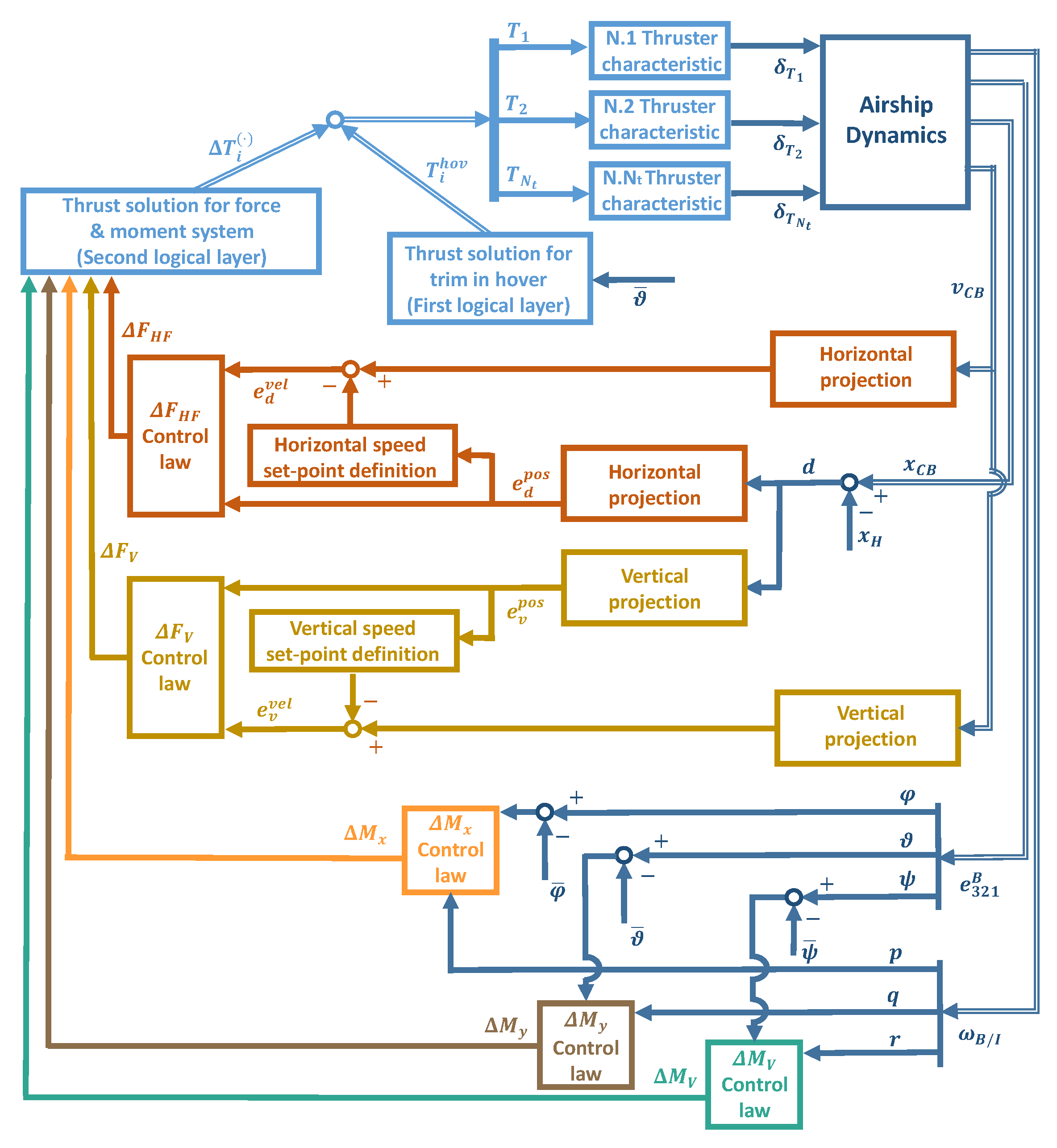
4. Control Schemes for Hover and Near-Hover

The analysis of equilibrium and of the control force systems introduced in the previous two paragraphs (Section 3.1 and Section 3.2) allows an effective thrust-based control scheme to be envisaged for hovering and near-hovering flight, without employing thrust-vector control.

The philosophy for the controller structure proposed herein is based on the concept that hover and near-hover control (HNHC) is an alternative stability augmentation and autonomous guidance mode with respect to forward flight control (FFC) mode. An effective implementation of a FFC mode for a thrust-controlled airship has been thoroughly described and discussed in a dedicated paper [16], showing its general effectiveness for stability augmentation and navigation tasks as well, and will not be treated here. The HNHC mode will be activated whenever hovering at a certain waypoint along a planned flight path is required. The physical transition from forward flight to hover (and from hover to forward flight as well) is managed within the HNHC mode. When activated for transitioning from forward flight to hover, the HNHC mode follows the logical scheme outlined below.

• The HNHC controller computes the thrust controls for hover $T_i^{\mathrm{hov}}$, $i=1,\dots ,N_t$, through the solution of Equations (9) and (10).
• Given the position of the airship wrt. the ground reference $\mathcal{I}$ (i.e., the coordinates in three-dimensional space), the HNHC controller computes the relative position vector $\mathit{d}=\left({\mathit{x}}_{\mathit{CB}}-{\mathit{x}}_{\mathit{H}}\right)$, between the target point for hover ${\mathit{x}}_{\mathit{H}}$ and the current position ${\mathit{x}}_{\mathit{CB}}$ (see plots on Figure 4).
• The airship is rolled to a null roll angle $\overline{\phi }=0$, by imposing values of $\Delta T_i^{\mathrm{roll}}$ required for a $\Delta M_x$ suitable for the task. These are computed as solutions of Equation (11), where all other components of the l.h.s. are set to zero, and from Equation (10).
• Concurrently, the airship is pitched to a target deck angle $\overline{\vartheta }$ by applying thrust components $\Delta T_i^{\mathrm{pitch}}$ to obtain a suitable $\Delta M_y$ (the same conceptual procedure as the previous point).
• The airship is steered around the vertical inertial axis ${\mathit{i}}_3$, to align the longitudinal body plane of symmetry with vector $\mathit{d}$, through a set of values $\Delta T_i^{\mathrm{yaw}}$ required for a suitable $\Delta M_V$ (the same conceptual procedure as the previous point).
• When alignment of the longitudinal plane of the airship with vector $\mathit{d}$ is reached within a certain tolerance, the airship is maneuvered through thrust force components $\Delta T_i^{\mathrm{HF}}$ and $\Delta T_i^{\mathrm{V}}$ equivalent to prescribed $\Delta F_{HF}$ and $\Delta F_V$ (the same conceptual procedure as the previous point), until the modulus of $\mathit{d}$ is satisfactorily small, i.e., the airship $\mathit{CB}$ is sufficiently close to the target point $\mathit{H}$. Then the airship is kept close to the target point by means of the same logic (i.e., horizontal-forward and vertical force).

A remark concerning the conceptual procedure just outlined is related to the non-use of horizontal-lateral force $\Delta F_{HL}$. This is clearly not a necessity, in case a lateral thrust force is available from the layout of the thrusters. However, from the second line in Equation (11), it is apparent that the only way to obtain $\Delta F_{HL}$ is from lateral components of thrust, which according to the second line in Equation (10) can be obtained only for a non-null angle ${\sigma }_i$. This means that, for granting a horizontal-lateral force in hover or near-hover, the thrusters should be mounted in a somewhat sidewards-tilted attitude. This is not a common choice, since it does not carry any particular advantage in forward flight [27]. Conversely, the presented philosophy copes with a configuration where ${\sigma }_i=0$, which is more commonly of practical interest.

Results on this configuration will be shown in Section 5 of the paper, witnessing good effectiveness of the proposed system, despite the lack of direct horizontal-lateral force control.

4.1. Control Laws for Stabilization and Guidance

Considering the controller architecture just outlined, equilibrium values of thrust in hover $T_i^{\mathrm{hov}}$ are obtained by direct computation, solving Equations (9) and (10). On the other hand, the components of thrust for stabilizing the airship and steering it in near-hover are obtained from a set of control forces and moments (through the solution of Equations (10) and (11)), which in turn need to be computed from corresponding feed-back loops. The two tasks of stabilization and guidance concur with the synthesis of the demand of control forces and moments. In particular, the following control laws are proposed.

• The rolling moment demand is obtained through a proportional law on the roll angle $\phi$ and roll component of the rotational speed of the airship p, as

  $$\Delta M_x=k_{\phi }\left(\phi -\overline{\phi }\right)+k_{p}p.$$

  (12)
  In Equation (12), the value of the reference roll can be set to zero, i.e., $\overline{\phi }=0$ as stated, to take (and keep) the airship around a null roll value (the equivalent of a leveler function on most autopilots of common winged aircraft). The rate-proportional component takes the function of a roll damper, to induce stable behavior around the roll axis.
• The pitching moment demand is obtained through a proportional law, acting on the pitch angle $\vartheta$ and on the pitching component of the rotational speed q, yielding

  $$\Delta M_y=k_{\vartheta }\left(\vartheta -\overline{\vartheta }\right)+k_{q}q,$$

  (13)

  where the value of $\overline{\vartheta }$ is a target deck angle in hover, set by the mission planner, for instance based on requirements concerning the attitude of the payload. In particular, the component proportional to the rotational rate takes on the role of the pitch stability augmentation system deployed in FFC mode, increasing the damping around the pitch axis.
• The moment demand in the ground-horizontal plane is regulated through a proportional control law with respect to a heading signal and a yaw damping effect is added through a feed-back of the yaw rate signal r. The feed-back variable for heading control is the heading error, defined as in the left plot of Figure 4. The ensuing control law yields

  $$\Delta M_V=k_{\psi }\left(\psi -\overline{\psi }\right)+k_{r}r,$$

  (14)

  where $\psi$ is the current heading of the airship.
• The values of $\Delta F_{HF}$ and $\Delta F_V$ demanded for position control are computed according to two independent, yet structurally similar, laws. These are based on a position error and a velocity error. The concept behind these laws is that the preliminary action of the heading alignment control (previous point), reducing the absolute value of the error $\psi -\overline{\psi }$ within a tolerance, will take the relative position vector $\mathit{d}$ on the longitudinal plane of the airship (or very close to this condition). From that condition, the horizontal-forward force $\Delta F_{HF}$ should act on the distance from the target on the local horizon plane, whereas $\Delta F_V$ should act only on the corresponding vertical distance. As already pointed out, no action outside of the longitudinal plane of the airship is required in this scenario. Analytically, the two laws can be written as

  $$\begin{array}{cc}\hfill \Delta F_{HF}=& k_d^{pos}{e}_d^{pos}+k_d^{vel}{e}_d^{vel},\hfill \\ \hfill \Delta F_V=& k_v^{pos}{e}_v^{pos}+k_v^{vel}{e}_v^{vel}.\hfill \end{array}$$

  (15)
  In Equation (15), the position errors are the distance error $e_d^{pos}$ and the vertical error $e_v^{pos}$, and they are pictorially defined on the right plot of Figure 4. Additionally, $e_d^{vel}$ and $e_v^{vel}$ are the velocity errors, respectively, between the velocity component on the local horizon plane or normal to it, and corresponding velocity set-points. The velocity set-points for horizontal and lateral speed are defined as functions of the corresponding position error, through a linear-bounded function. In particular, the velocity set-points are limited between a top and bottom value, which are reached for assigned values of the position errors, whereas the velocity set-points are null when the corresponding position errors are null.

The flowchart of the control architecture is shown in Figure 5. Additionally, some of the gains are managed as functions of other variables. In particular, the heading error $|\psi -\overline{\psi }|$ and the position error $\left|\mathit{d}\right|$ are employed as supervision variables. Out of close proximity to the target, i.e., $\left|\mathit{d}\right|>d_{min}$, with $d_{min}$ empirically set to a value below the half length of the envelope, the airship is steered first to achieve alignment $|\psi -\overline{\psi }| < \Delta {\psi }_{max}$. Until alignment has been reached, $\Delta F_{HF}$, $\Delta F_V$ and $\Delta M_y$ operate only through damping control laws, i.e., without the components proportional to angles or positions (see Equations (13) and (14)), but only those proportional to rates or velocities, which are invariably drawn to zero (damping action). Conversely, when the airship heading is within the alignment error threshold $\Delta {\psi }_{max}$, the control laws for $\Delta F_{HF}$, $\Delta F_V$ and $\Delta M_y$ are fully activated.

Upon entering close proximity to the target position, i.e., $\left|\mathit{d}\right| \le d_{min}$, $\Delta M_x$ and $\Delta M_V$ control demand components proportional to angles are inhibited, and the loops in Equations (12) and (14) act proportionally to rates, providing a damping action around the rolling and yawing axes. Inhibiting feed-back of the heading error when in close proximity to the target is desirable, to avoid control divergence in case of a slight lateral position inaccuracy between the airship longitudinal plane and the target point. Of course, irrespective of heading error, within the $d_{min}$ distance threshold $\Delta M_y$, $\Delta F_{HF}$ and $\Delta F_V$ in Equations (13) and (15) control loops are fully operative. This scheme implicitly assumes accepting a limited steady state error in terms of a lateral displacement between the longitudinal plane of the airship and the target point. However, the boundary on such error can be set through the $\Delta {\psi }_{max}$ and $d_{min}$ values, according to the accuracy requirements of the hovering phase.

4.2. Additional Remarks on Control Laws

A remark concerns the choice of the reference value of the roll angle $\overline{\phi }$. As just pointed out, satisfactory results can be obtained setting this value to zero. However, it was found that a slight improvement in the time needed for alignment (i.e., for reducing $|\psi -\overline{\psi }|$ below $\Delta {\psi }_{max}$) can be obtained by targeting the side-slip motion in near-hover, i.e., the component of velocity V out of the longitudinal plane of the airship. As observed, a scenario where no lateral thrust is available is considered of interest. In that setting, a side force $\Delta F_{HL}$ in the local horizontal plane can still be obtained, by slightly rolling the airship and concurrently imposing a vertical force in the longitudinal plane, thus yielding a $\Delta F_{HL}^{{}^{\prime }}={\sum }_{i=1}^{N_t}\left(\Delta T_{i_z}sin\phi \right)$. The demand of this further control component can be defined through a dedicated control loop, such that $\Delta F_{HL}^{{}^{\prime }}=k_{V}V$, thus targeting the value of the side-slip speed. This yields a further set of thrust setting requirements $\Delta T_i^{H{L}^{{}^{\prime }}}$, obtained from Equation (10).

Since this control is employed for refining the major control action already carried out by the architecture just described, which is based on a null roll among its basic hypotheses (in particular, Equations (9) and (11) are obtained through that hypothesis, as pointed out), the target roll angle $\overline{\phi }$ will take a very limited value. In the proposed implementation, this target value has been managed as a linear-bounded function of the measured lateral speed V and the gain $k_V$ has been set to a very small value compared to the other gains in the roll control law (Equation (12)).

A final consideration on the proposed architecture is related to wind. The HNHC control mode, as stated, has been considered as an alternative to the FFC mode for forward flight. The implementation proposed for the latter with application to a thrust-controlled airship, introduced in [16], has been proved capable of dealing with steady wind fields with non-negligible intensity. Furthermore, from a conceptual flight dynamics and control standpoint, an airship trying to perform station keeping in presence of a significant wind is a control problem closer to navigation in forward flight than a near-hover or hover condition. For instance, the fins will be effective as stabilizers, whereas steering the airship out of the wind, when at all possible, would require a significant engagement of the controls. These effects are due to the fact that aerodynamic actions are non-negligible when a significant wind is acting on the airship, thus hampering the adoption of the hypotheses yielding the equilibrium equation for hover, Equation (8). Correspondingly, the scheme just introduced for control in hover and near-hover is not intended/suitable to cover that type of flight, i.e., a station keeping forward flight, which may be, however, dealt with successfully through slight modifications to the FFC navigation mode.

In the proposed implementation, as pointed out, the FFC and HNHC are alternative modes, and the latter is activated under a threshold airspeed, i.e., when $|{\mathit{v}}_{\mathit{CB}}| \le v_{thr}$. This threshold has been identified empirically in case studies, starting from a forward flight condition and reducing the advance speed set-point while a satisfactory reaction to disturbances is still obtained. When this does not happen any more, due to the inherent loss of stability due to the ineffectiveness of the stabilizing fins, a limit for the FFC applicability has been reached. The threshold speed is then set suitably above that value.

4.3. From Force and Moment Demands to Thrust Settings

When online, the controller computes the reference values of thrust force for hover, and the demanded steering actions (forces and moments), required for the hover and near-hover navigation tasks at every time instant.

Reference values of thrust $T_i^{\mathrm{hov}}$ for $i=1,\dots ,N_t$, can be computed for hover from the systems in Equations (9) and (10), having assigned the needed geometrical quantities and the reference deck angle ${\vartheta }_0=\overline{\vartheta }$.

Concurrently, once the force and moment demands from the branches of the controller (Figure 5) have been computed in terms of required values of $\Delta F_{HF}$, $\Delta F_V$ and $\Delta F_{HL}^{{}^{\prime }}$ (if any), $\Delta M_x$, $\Delta M_y$ and $\Delta M_V$, equivalent components of thrust force $\Delta T_i^{\mathrm{roll}}$, $\Delta T_i^{\mathrm{pitch}}$, $\Delta T_i^{\mathrm{yaw}}$ and $\Delta T_i^{H{L}^{{}^{\prime }}}$ (if any), $\Delta T_i^{\mathrm{V}}$, $\Delta T_i^{\mathrm{HF}}$, $i=1,\dots ,N_t$, can be computed starting from the lines in Equation (11) and again Equation (10) (where symbol $T_i$ has been substituted by $\Delta T_i$).

These passages yield the final thrust control demand at the current instant, which can be written as

$$T_i=T_i^{\mathrm{hov}}+\Delta T_i^{\mathrm{roll}}+\Delta T_i^{\mathrm{pitch}}+\Delta T_i^{\mathrm{yaw}}+\Delta T_i^{\mathrm{HF}}+\Delta T_i^{\mathrm{V}}.$$

(16)

The overall thrust contribution $T_i$ for each thruster in Equation (16) is finally turned into a control demand ${\delta }_{T_i}$. The latter, computed for $i=1,\dots ,N_t$, produces the current value of the control array ${\mathit{u}}^t$. The computation of ${\delta }_{T_i}$ is conceptually performed solving the characteristic equation Equation (7). However, since thruster performance data are typically known in practice through a lookup table, the number of operations for this step in the procedure is always the same; hence, a predictable and constant computational passage is required for physically converting the thrust force demand $T_i$ into a ${\delta }_{T_i}$ control signal, to be sent to the corresponding actuator.

Results from the application of the presented control scheme will be presented in association with a case study in the next section.

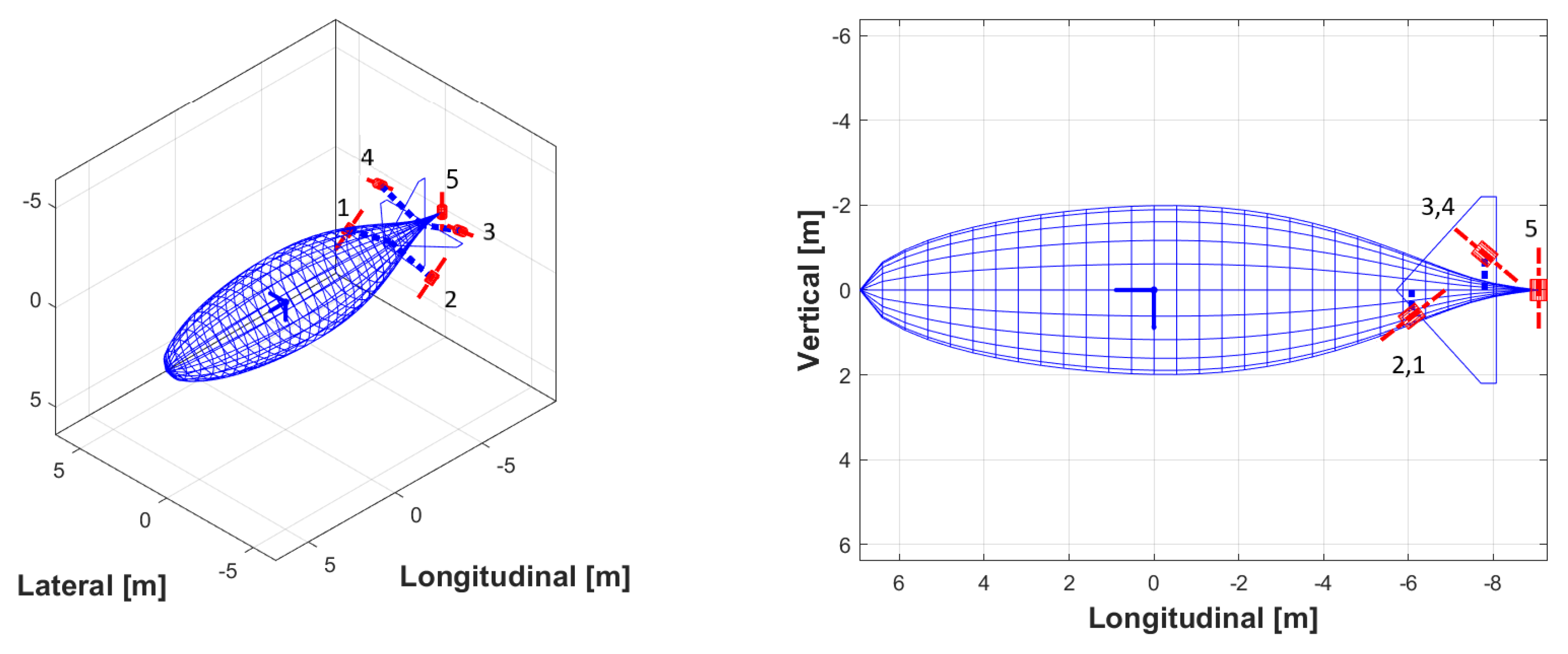
5. Case Study: A Five-Thruster Thrust-Controlled Airship

In this section, example results obtained from the application of the control scheme introduced in the previous paragraphs are proposed. The control architecture has been applied to the virtual model of a thrust-controlled airship concept, designed starting from the envelope and general sizing of the Lotte airship [11,12], and previously employed for similar studies [16,27]. In particular, a slight modification to previous versions of the conceptual thrust-based test-bed is the addition of a fifth auxiliary thruster, positioned on the tail cone and with a thrust line parallel to the vertical body axis of the airship. Basic data for the test-bed are reported in

Table 1. Reference data for the considered airship test-bed.

Parameter		Value
Mass m (kg)		137.28
Envelope volume $Vol$ (m3)		107.42
Overall length (m)		16.0
Horizontal displacement of $\mathit{CG}$ from $\mathit{CB}$,  $r_{{\mathit{CG}}_x}$ (m)		0.006
Vertical displacement of $\mathit{CG}$ from $\mathit{CB}$,  $r_{{\mathit{CG}}_z}$ (m)		0.455
Number of thrusters $N_t$		5
Nominal thrust ${\tilde{T}}_i$ (each unit) (N)		250
Pos. of Nr. 1 thruster wrt. $\mathit{CB}$,  $\left\{r_{{\mathit{P}}_{{\mathit{T}}_{1_x}}},r_{{\mathit{P}}_{{\mathit{T}}_{1_y}}},r_{{\mathit{P}}_{{\mathit{T}}_{1_z}}}\right\}$ (m)		$\left\{-5.262,2.309,0.731\right\}$
Pos. of Nr. 2 thruster wrt. $\mathit{CB}$,  $\left\{r_{{\mathit{P}}_{{\mathit{T}}_{2_x}}},r_{{\mathit{P}}_{{\mathit{T}}_{2_y}}},r_{{\mathit{P}}_{{\mathit{T}}_{2_z}}}\right\}$ (m)		$\left\{-5.262,-2.309,0.731\right\}$
Pos. of Nr. 3 thruster wrt. $\mathit{CB}$,  $\left\{r_{{\mathit{P}}_{{\mathit{T}}_{3_x}}},r_{{\mathit{P}}_{{\mathit{T}}_{3_y}}},r_{{\mathit{P}}_{{\mathit{T}}_{3_z}}}\right\}$ (m)		$\left\{-5.877,-2.221,-0.855\right\}$
Pos. of Nr. 4 thruster wrt. $\mathit{CB}$,  $\left\{r_{{\mathit{P}}_{{\mathit{T}}_{4_x}}},r_{{\mathit{P}}_{{\mathit{T}}_{4_y}}},r_{{\mathit{P}}_{{\mathit{T}}_{4_z}}}\right\}$ (m)		$\left\{-5.877,2.221,-0.855\right\}$
Pos. of Nr. 5 thruster wrt. $\mathit{CB}$,  $\left\{r_{{\mathit{P}}_{{\mathit{T}}_{5_x}}},r_{{\mathit{P}}_{{\mathit{T}}_{5_y}}},r_{{\mathit{P}}_{{\mathit{T}}_{5_z}}}\right\}$ (m)		$\left\{-9.07,0,0\right\}$
Thruster tilt angle ${\lambda }_1={\lambda }_2$ (deg)		34.7
Thruster tilt angle ${\lambda }_3={\lambda }_4$ (deg)		−38.7
Thruster tilt angle ${\lambda }_5$ (deg)		90
Thruster side angle ${\sigma }_1={\sigma }_2={\sigma }_3={\sigma }_4={\sigma }_5$ (deg)		0

and a sketch is presented in Figure 6. In particular, thrusters 1 to 4 are numbered from the bottom right in a clockwise direction, looking at the airship from the back (as in [16]), and thruster Nr. 5 is the tail thruster. A positive value of ${\lambda }_i$ corresponds to a downward tilt, according to Figure 2.

Notably, the longitudinal position of the center of gravity $\mathit{CG}$ differs from that of the center of buoyancy $\mathit{CB}$. This implies that this airship, when hypothetically controlled only through the action of aerodynamic surfaces, would be impossible to trim with a null (or arbitrary) deck angle in hover. Conversely, hover equilibrium would be obtained with a deck angle such as to take the horizontal displacement of $\mathit{CG}$ and $\mathit{CB}$ to zero (which might correspond to a severe tip-over tendency of the airship when parked or in hovering flight at an assigned deck angle). This is a well-known issue on airships, typically solved with suitably positioned balancing dead-weights. As will be soon demonstrated and observed through practical analyses, the longitudinal displacement of $\mathit{CG}$ and $\mathit{CB}$ can be managed in the thrust-controlled configuration here presented, granting trimmability in hover with no dead-weights, at an arbitrary deck angle. This is possible since the thrusters do not lose their authority in hover, differently from aerodynamic surfaces.

A high-fidelity model of the airship dynamics has been implemented in SILCROAD [16], taking into account fully non-linear flight dynamics and the accurate layout of all thrusters. Concerning the thrusters, an assembly of a propeller driven by an electric motor was considered conceptually for each of them. A first-order system with a time constant of 0.001 s has been considered as a model, on account of a generally fast response of electric motors. Referring to Equation (7), the output thrust of thrusters saturates at the value of thrust reached for ${\delta }_{T_i}=\pm$1 and is modulated by the input ${\delta }_{T_i}$ through a value ${\tilde{K}}_i\left({\delta }_{T_i}\right)$ defined as follows [27]

$${\tilde{K}}_i\left({\delta }_{T_i}\right)=\left\{\begin{array}{cc}1.0,& {\delta }_{T_i}\ge 0\\ -0.5,& {\delta }_{T_i}<0\end{array}\right.,$$

(17)

where the modulation in Equation (17) was employed to coarsely model the loss in efficiency of a propeller working in the opposite direction with respect to the intended one.

5.1. Assessment of Thruster Layout: Trim in Hover and Steering in Near-Hover

As mentioned in Section 3.1 and Section 3.2, the systems in Equations (9)–(11) (properly combined as shown) do not universally bear a solution. In particular, the very existence of a solution requires a suitable layout of the thrusters on board the airship. It is interesting to specialize these systems of linear equations for the case of the test-bed considered in this work, to show that in this case they bear well-posed mathematical problems, thus allowing the successful deployment of the proposed control architecture.

5.1.1. Control Solution for Trim in Hover

Considering the layout shown in Figure 6, in the hover equilibrium represented by Equation (9) the l.h.s. is formally unchanged, whereas the r.h.s. can be assigned as

$$\left\{\begin{array}{cccc}\hfill (m-\rho Vol)gsin{\vartheta }_0=& T_{1_x}+T_{2_x}+T_{3_x}+T_{4_x},\hfill & \hfill & \mathrm{lon}.\mathrm{force}\mathrm{eql}.\hfill \\ \hfill -(m-\rho Vol)gcos{\vartheta }_0=& T_{1_z}+T_{2_z}+T_{3_z}+T_{4_z}+T_{5_z},\hfill & \hfill & \mathrm{ver}.\mathrm{force}\mathrm{eql}.\hfill \\ \hfill 0=& (T_{1_z}-T_{2_z})r_{{\mathit{P}}_{{\mathit{T}}_{1_y}}}+(-T_{3_z}+T_{4_z})r_{{\mathit{P}}_{{\mathit{T}}_{4_y}}},\hfill & \hfill & \mathrm{rol}.\mathrm{mom}.\mathrm{eql}.\hfill \\ \hfill mg\left(r_{{\mathit{CG}}_z}sin{\vartheta }_0+r_{{\mathit{CG}}_x}cos{\vartheta }_0\right)=& (T_{1_x}+T_{2_x})r_{{\mathit{P}}_{{\mathit{T}}_{1_z}}}+(T_{3_x}+T_{4_x})r_{{\mathit{P}}_{{\mathit{T}}_{4_z}}}\hfill & \hfill & \\ \hfill & -(T_{1_z}+T_{2_z})r_{{\mathit{P}}_{{\mathit{T}}_{1_x}}}-(T_{3_z}+T_{4_z})r_{{\mathit{P}}_{{\mathit{T}}_{4_x}}}-T_{5_z}{r}_{{\mathit{P}}_{{\mathit{T}}_{5_x}}},\hfill & \hfill & \mathrm{pit}.\mathrm{mom}.\mathrm{eql}.\hfill \\ \hfill 0=& (-T_{1_x}+T_{2_x})r_{{\mathit{P}}_{{\mathit{T}}_{1_y}}}+(T_{3_x}-T_{4_x})r_{{\mathit{P}}_{{\mathit{T}}_{4_y}}}.\hfill & \hfill & \mathrm{yaw}.\mathrm{mom}.\mathrm{eql}.\hfill \end{array}\right.$$

(18)

The balance of the linear system in Equation (18) yields five equations in the nine unknowns $T_{1_x}$, $T_{2_x}$, $T_{3_x}$, $T_{4_x}$, $T_{1_z}$, $T_{2_z}$, $T_{3_z}$, $T_{4_z}$ and $T_{5_z}$. In particular, the values of $T_{i_y}$, $i=1,\dots ,5$ have been purged together with the second line in the system of Equation (9), since it turns trivial in the current configuration, where no lateral body components of thrust exist. The system in Equation (18) is then flanked by the following writing of Equation (10), specialized for the case of the five-thruster configuration of interest, yielding

$$\left\{\begin{array}{ccccccccc}\hfill T_{1_x}=T_{1}cos{\lambda }_1,& \hfill & \hfill T_{2_x}=T_{2}cos{\lambda }_1,& \hfill & \hfill T_{3_x}=T_{3}cos{\lambda }_4,& \hfill & \hfill T_{4_x}=T_{4}cos{\lambda }_4,& \hfill & \\ \hfill T_{1_z}=T_{1}sin{\lambda }_1,& \hfill & \hfill T_{2_z}=T_{2}sin{\lambda }_1,& \hfill & \hfill T_{3_z}=T_{3}sin{\lambda }_4,& \hfill & \hfill T_{4_z}=T_{4}sin{\lambda }_4,& \hfill & \hfill T_{5_z}=T_5.\end{array}\right.$$

(19)

The system in Equation (19) adds nine equations and five more unknowns, namely the thrust intensities $T_1$, $T_2$, $T_3$, $T_4$ and $T_5$. Together, the systems in Equations (18) and (19) produce a set of 14 linear equations in 14 unknowns. Except for extreme choices of ${\lambda }_1$, ${\lambda }_4$ and ${\vartheta }_0$, or of the positions of the thrusters relative to the $\mathit{CB}$ (i.e., values of $r_{{\mathit{P}}_{{\mathit{T}}_{i_x}}}$, $r_{{\mathit{P}}_{{\mathit{T}}_{i_y}}}$ and $r_{{\mathit{P}}_{{\mathit{T}}_{i_z}}}$) yielding a singular system and hampering the obtainment of a solution, from Equations (18) and (19) it is possible to obtain a closed-form solution in terms of $T_i$, $i=1,\dots ,5$, to implement in a control algorithm on board. In particular, with the data presented in Table 1 and in Figure 6, a closed-form solution to this linear system exists, yielding the values of $T_i^{\mathrm{hov}}$ needed for hover, which are also employed as a reference in near-hovering flight (Equation (16)).

To stress further the relevance of a suitable choice of the layout of the thrusters, it should be noted that the addition of the fifth thruster on the tail, with a body-vertical line of thrust (i.e., ${\lambda }_5=90$ deg), is needed and sufficient for correctly posing the system for trimmed flight in hover, starting from the original four-thruster configuration studied in [16,27]. Actually, considering taking away that thruster, as in the original configuration optimized for forward flight, the system (Equations (18) and (19)) would lose two unknowns (i.e., $T_{5_z}$ and $T_5$) but only one equation (i.e., $T_{5_z}=T_5$), yielding an ill-posed, over-constrained problem. Therefore, as anticipated in Section 3.1, a preliminary choice of the layout of the thrusters is a substantial step towards granting the existence of a trimmed control solution for the airship in hover.

5.1.2. Steering Control in Near-Hover

Considering now the system in Equation (11), it can be specialized to the case of the five-thruster configuration at hand as follows,

$$\left\{\begin{array}{cccc}\hfill \Delta F_{HF}=& \left(\Delta T_{1_x}+\Delta T_{2_x}+\Delta T_{3_x}+\Delta T_{4_x}\right)cos\vartheta \hfill & \hfill & \\ & +\left(\Delta T_{1_z}+\Delta T_{2_z}+\Delta T_{3_z}+\Delta T_{4_z}+\Delta T_{5_z}\right)sin\vartheta \hfill & \hfill & \mathrm{hor}.-\mathrm{for}.\mathrm{force}\mathrm{comp}.\hfill \\ \hfill \Delta F_V=& -\left(\Delta T_{1_x}+\Delta T_{2_x}+\Delta T_{3_x}+\Delta T_{4_x}\right)sin\vartheta \hfill & \hfill & \\ & +\left(\Delta T_{1_z}+\Delta T_{2_z}+\Delta T_{3_z}+\Delta T_{4_z}+\Delta T_{5_z}\right)cos\vartheta \hfill & \hfill & \mathrm{ver}.\mathrm{force}\mathrm{comp}.\hfill \\ \hfill \Delta M_x=& \left(\Delta T_{1_z}-\Delta T_{2_z}\right)r_{{\mathit{P}}_{{\mathit{T}}_{1_y}}}+\left(-\Delta T_{3_z}+\Delta T_{4_z}\right)r_{{\mathit{P}}_{{\mathit{T}}_{4_y}}},\hfill & \hfill & \mathrm{rol}.\mathrm{mom}.\mathrm{comp}.\hfill \\ \hfill \Delta M_y=& \left(\Delta T_{1_x}+\Delta T_{2_x}\right)r_{{\mathit{P}}_{{\mathit{T}}_{1_z}}}+\left(\Delta T_{3_x}+\Delta T_{4_x}\right)r_{{\mathit{P}}_{{\mathit{T}}_{4_z}}}\hfill & \hfill & \\ & -\left(\Delta T_{1_z}+\Delta T_{1_z}\right)r_{{\mathit{P}}_{{\mathit{T}}_{1_x}}}-\left(\Delta T_{3_z}+\Delta T_{4_z}\right)r_{{\mathit{P}}_{{\mathit{T}}_{4_x}}}-\Delta T_{5_z}{r}_{{\mathit{P}}_{{\mathit{T}}_{5_x}}},\hfill & \hfill & \mathrm{pit}.\mathrm{mom}.\mathrm{comp}.\hfill \\ \hfill \Delta M_V=& -\left(\left(\Delta T_{1_x}-\Delta T_{2_x}\right)cos\vartheta +\left(\Delta T_{1_z}-\Delta T_{2_z}\right)sin\vartheta \right)r_{{\mathit{P}}_{{\mathit{T}}_{1_y}}}\hfill & \hfill & \\ & -\left(\left(-\Delta T_{3_x}+\Delta T_{4_x}\right)cos\vartheta +\left(-\Delta T_{3_z}+\Delta T_{4_z}\right)sin\vartheta \right)r_{{\mathit{P}}_{{\mathit{T}}_{4_y}}},\hfill & \hfill & \mathrm{mom}.\mathrm{hor}.\mathrm{plane}\mathrm{comp}.\hfill \end{array}\right.$$

(20)

where the components of $\Delta T_i$ are defined as follows,

$$\left\{\begin{array}{ccccccccc}\hfill \Delta T_{1_x}=\Delta T_{1}cos{\lambda }_1,& \hfill & \hfill \Delta T_{2_x}=\Delta T_{2}cos{\lambda }_1,& \hfill & \hfill \Delta T_{3_x}=\Delta T_{3}cos{\lambda }_4,& \hfill & \hfill \Delta T_{4_x}=\Delta T_{4}cos{\lambda }_4,& \hfill & \\ \hfill \Delta T_{1_z}=\Delta T_{1}sin{\lambda }_1,& \hfill & \hfill \Delta T_{2_z}=\Delta T_{2}sin{\lambda }_1,& \hfill & \hfill \Delta T_{3_z}=\Delta T_{3}sin{\lambda }_4,& \hfill & \hfill \Delta T_{4_z}=\Delta T_{4}sin{\lambda }_4,& \hfill & \hfill \Delta T_{5_z}=\Delta T_5.\end{array}\right.$$

(21)

Similarly to the case of hover equilibrium examined previously in this section, the 14 equations in Equations (20) and (21) produce a linear system in the 14 unknowns $\Delta T_{1_x}$, $\Delta T_{2_x}$, $\Delta T_{3_x}$, $\Delta T_{4_x}$, $\Delta T_{1_z}$, $\Delta T_{2_z}$, $\Delta T_{3_z}$, $\Delta T_{4_z}$ and $\Delta T_{5_z}$, as well as $\Delta T_1$, $\Delta T_2$, $\Delta T_3$, $\Delta T_4$ and $\Delta T_5$. The same considerations made for equilibrium in hover on well-posing the system through a suitable layout of the thrusters apply also here.

Referring to the control logical procedure introduced in Section 4, for each of the cited control actions (e.g., exerting rolling moment, pitching moment, etc.), a corresponding l.h.s. of the system in Equation (20) is obtained, where only one demanded action is non-null and all others are null. Correspondingly, the thrust forces on the r.h.s. of Equation (16) are obtained.

Morevoer, it may be observed that, exploiting the linearity of the system, the superimposition of the solutions to each of the so-configured systems is a solution as well. In other words, considering a single system where all required forces and moments appear simultaneously on the l.h.s. of Equation (20), a solution is obtained which is the superimposition of the solutions obtained from the systems where only one action at a time is non-null on the l.h.s. of the system. Therefore, the separate definition of the control actions on the r.h.s. of Equation (16) (corresponding to rolling moment, pitching moment, etc.) is not strictly needed at an implementation level but helps clarity in the explanation.

5.2. Numerical Results

Numerical results from time-marching simulations on the virtual test-bed are presented in this section. At first, transition from forward flight to hover is analyzed without requirements for station keeping at an assigned position. Then, two near-hovering and hovering missions, including station keeping at an assigned position, are analyzed, to better appreciate the abilities of the different functions of the proposed control architecture.

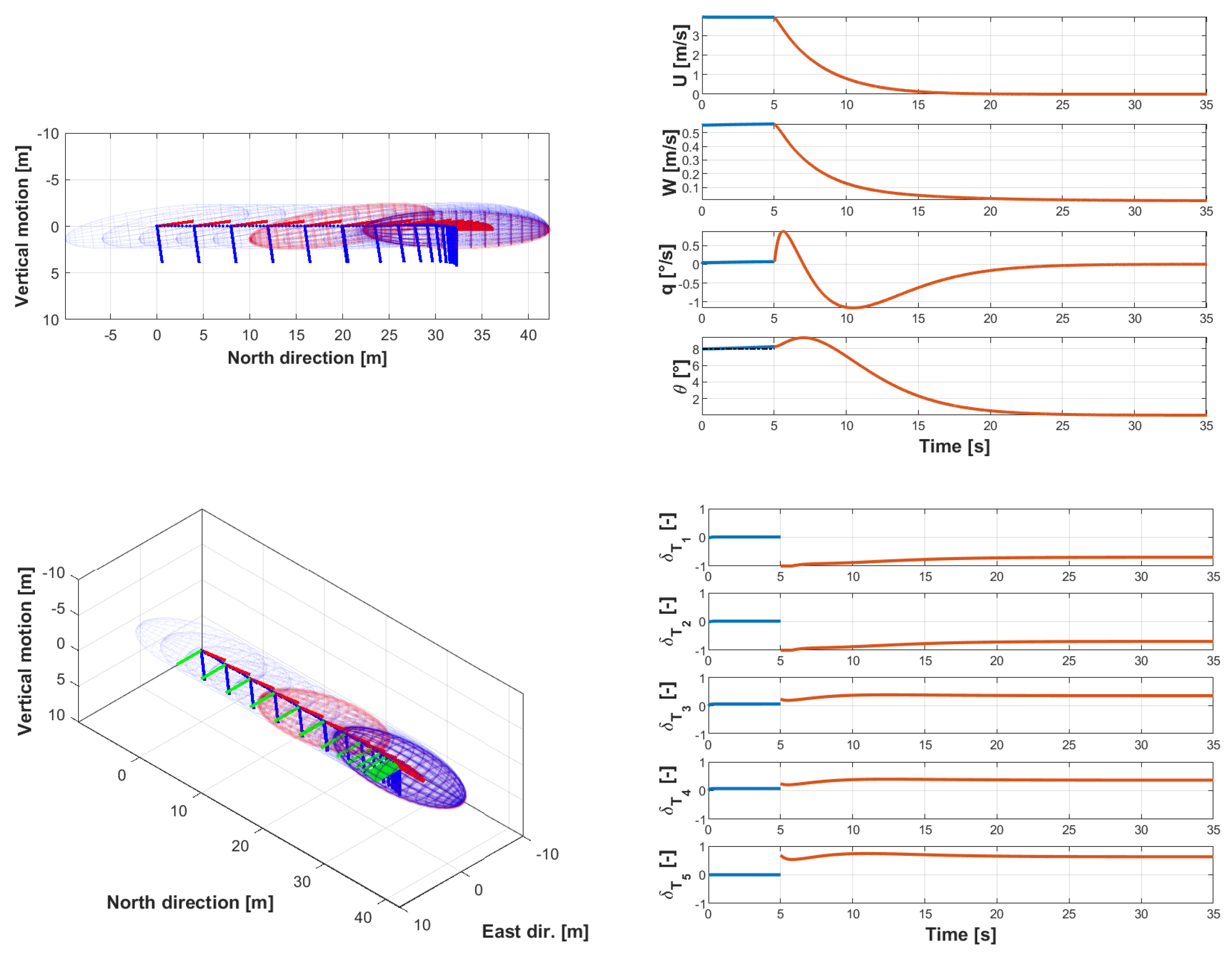
5.2.1. Transition from Forward Flight to a Hovering Condition

In this trial, the ability of the HNHC mode to manage an arrest of the airship without any diverging behavior in its state is demonstrated.

The simulation starts with the airship trimmed in forward flight at 4 m/s (which has been set as $v_{thr}$ for this airship). Upon reaching a checkpoint at the end of the navigation phase, the HNHC mode is activated without a specific target position to keep. This implies that the angle $\psi$ is not controlled, nor the final position with respect to the ground inertial frame $\mathcal{I}$. Furthermore, the controller acts towards a null velocity set-point, thus towards a damping of translation, a null roll set-point ($\overline{\phi }=0$ deg) and a target $\overline{\vartheta }=0$ deg. In analytic terms, this scenario is described with the control laws in Equations (12) and (13) fully working, the gain $k_{\psi }=0$ in Equation (14) and gains $k_d^{pos}=k_v^{pos}=0$ in Equation (15). In the latter, the reference values for both horizontal and vertical speed in $e_d^{vel}$ and $e_v^{vel}$ are zero, so that $\Delta F_{HF}$ and $\Delta F_V$ are employed to achieve pure damping.

The top-left plot and bottom-left plots in Figure 7 show the resulting trajectory, looking at the airship from the right-hand side (top) and in a three-quarters view (bottom). A synthetic three-dimensional representation of the traveling airship is shown, as well as the corresponding body frame position and attitude (red: longitudinal axis ${\mathit{b}}_1$, green: right-hand axis ${\mathit{b}}_2$, blue: vertical axis ${\mathit{b}}_3$). The airship starts at zero coordinates and travels in FFC mode in horizontal steady flight for 20 m (marked by a red-painted airship in the plots). Then the HNHC mode is activated, with the peculiar settings just pointed out. The airship is effectively slowed down and the deck angle is tilted down from the initial value $\vartheta$ required for equilibrium in forward flight to the desired $\overline{\vartheta }=0$ deg. Hover is achieved when the airship is not traveling or rotating. From the top-right plot in Figure 7, speed components are null at around $t=20$ s. This means that the airship can be arrested starting from a forward speed of 4 m/s in about 15 s. About 5 s more are employed for achieving the target $\overline{\vartheta }$ value, which is reached at around $t=25$ s.

Looking at the trajectory from the side (top-left plot), a forward travel of about 12 m and an altitude decrease of slightly less than 1 m are obtained during the slow-down maneuver. This is the result of the inhibition of position control in this specific analysis. Clearly, to achieve better precision, the position-tracking loops already described need to be activated (addressed in the following test cases).

The bottom-right plot in Figure 7 shows the behavior of controls ${\delta }_{T_i}$. The discontinuity of the control history is due to the commutation from the forward flight (FFC) to the hover and near-hover control (HNHC) mode. Notably, the solution for forward flight does not require the employment of the fifth thruster, in accordance with the findings of previous works by the authors [16,27]. Interestingly, the control solution for hover is significantly different from that required for forward flight and is based on a relatively intense action from the thrusters in steady state (reached towards the end of the simulation). Looking at the control solution for hover in detail, it is possible to note that the settings of the bottom thrusters ${\delta }_{T_1}$ and ${\delta }_{T_2}$ (obviously equal in a symmetric flight condition) are significantly negative, yielding an upward and backward thrust component, and a corresponding pitch-down moment is obtained. The settings of the top thrusters ${\delta }_{T_3}$ and ${\delta }_{T_4}$ (again, mutually equal) are positive, corresponding to an upward and forward force component, and again a resulting pitch-down contribution to moment. The backward and forward components from top and bottom thrusters compensate each other, whereas a significant overall upwards force results from these four thrusters, and correspondingly a pitch-down moment. The vertical force from these four thrusters exceeds the need for vertical stationing for this airship. Actually, the vertically oriented tail thruster erodes much of this vertical contribution, through a significantly positive ${\delta }_{T_5}$, i.e., a strong downward force. The latter brings equilibrium, reducing total vertical thrust to the correct level and balancing the overall pitching moment on the airship, by producing a significant pitch-up contribution.

The solution just described clearly employs much of the range of the actuators for static equilibrium in hover (i.e., for producing the correct $T_i^{\mathrm{hov}}$), leaving a relatively reduced range for near-hover steering and for stability augmentation. In this particular case, saturation is encountered only briefly, soon after the activation of the HNHC mode (bottom-right plot in Figure 7) and apparently does not bear a significant detrimental effect on the overall performance of the HNHC mode.

5.2.2. From forward Flight to Hover at Assigned Position-Longitudinal Motion

A second case is presented, where the airship starts from the same condition as in the previous one (Section 5.2.1), i.e., a forward flight navigation at 4 m/s. Upon reaching a navigation check-point located 20 m north from the starting position, the HNHC mode is enabled, and a hovering condition at a point 15 m further ahead and 5 m up in altitude is set as a target for station keeping. Simultaneously, a reduction of the deck angle to $\overline{\vartheta }=0$ deg is requested.

The tolerance in terms of position accuracy is set so that the $\mathit{CB}$ of the airship keeps within a sphere with a diameter of 0.5 m around the target point, with a very restrictive top residual velocity (modulus) of 0.001 m/s.

Given the longitudinal symmetry of the problem, there is no stimulation of the lateral directional control laws. However, the complete control system (Equations (12)–(15)) is active. In particular, concerning the linear bounded functions defining the forward and vertical speed set-points (which in turn contribute to $e_d^{vel}$ or $e_v^{vel}$), they are such that the speed set-point modulus is 0.3 m/s for a displacement error (either $e_d^{pos}$ or $e_v^{pos}$) reaching or passing 0.5 m, whereas the set-point is linearly reduced to 0 m/s when the displacement error approaches 0 m.

The top-left plot in Figure 8 displays the motion of the airship seen from the right-hand side. In particular, the plot isolates the travel from the end-of-navigation check-point (the black sphere and the red-painted airship emerging from the left) and the target point for hover (marked by the black sphere at 35 m on the horizontal axis and 5 m above the zero on the vertical axis). Upon reaching the former, the HNHC mode is activated.

The bottom-left plot displays the time evolution of the longitudinal motion (which unfolds in the northern direction with respect to the ground frame $\mathcal{I}$) and the vertical displacement (wrt. $\mathcal{I}$). The dashed horizontal lines represent the amplitude of the tolerance range, around both the end-of-navigation check-point and the target point for hover. The behavior of the system piloted by the HNHC is generally satisfactory, with a mild overshoot of the target position, which is recovered reasonably fast to within a realistically acceptable precision tolerance (and even within the imposed strict tolerance values in a globally limited time) and without significant oscillations. Concurrently, the deck angle is successfully drawn to the desired horizontal condition.

The behavior of longitudinal states and of thrust control settings is shown in Figure 8, respectively on the top-right and bottom-right plots. On the former, the convergence history of the deck angle is portrayed through $\vartheta$ and q, showing a generally smooth and steadily converging behavior when the HNHC is engaged, despite the initial pitch-up elongation. The latter can be explained looking at the time history of controls (bottom-right), where saturation is encountered for a significant time range immediately following the engagement of the HNHC, especially on the bottom thrusters (${\delta }_{T_1}$ and ${\delta }_{T_2}$). Despite recovery without particular divergence issues in the near-hover navigation phase, as pointed out in Section 5.2.1 this may suggests the need for more control range (i.e., higher ${\tilde{T}}_i$) or conversely for less intense gains, which, however, will reduce the rate of convergence to the desired stationing position, requiring a longer time for settling within an acceptable displacement tolerance from the target.

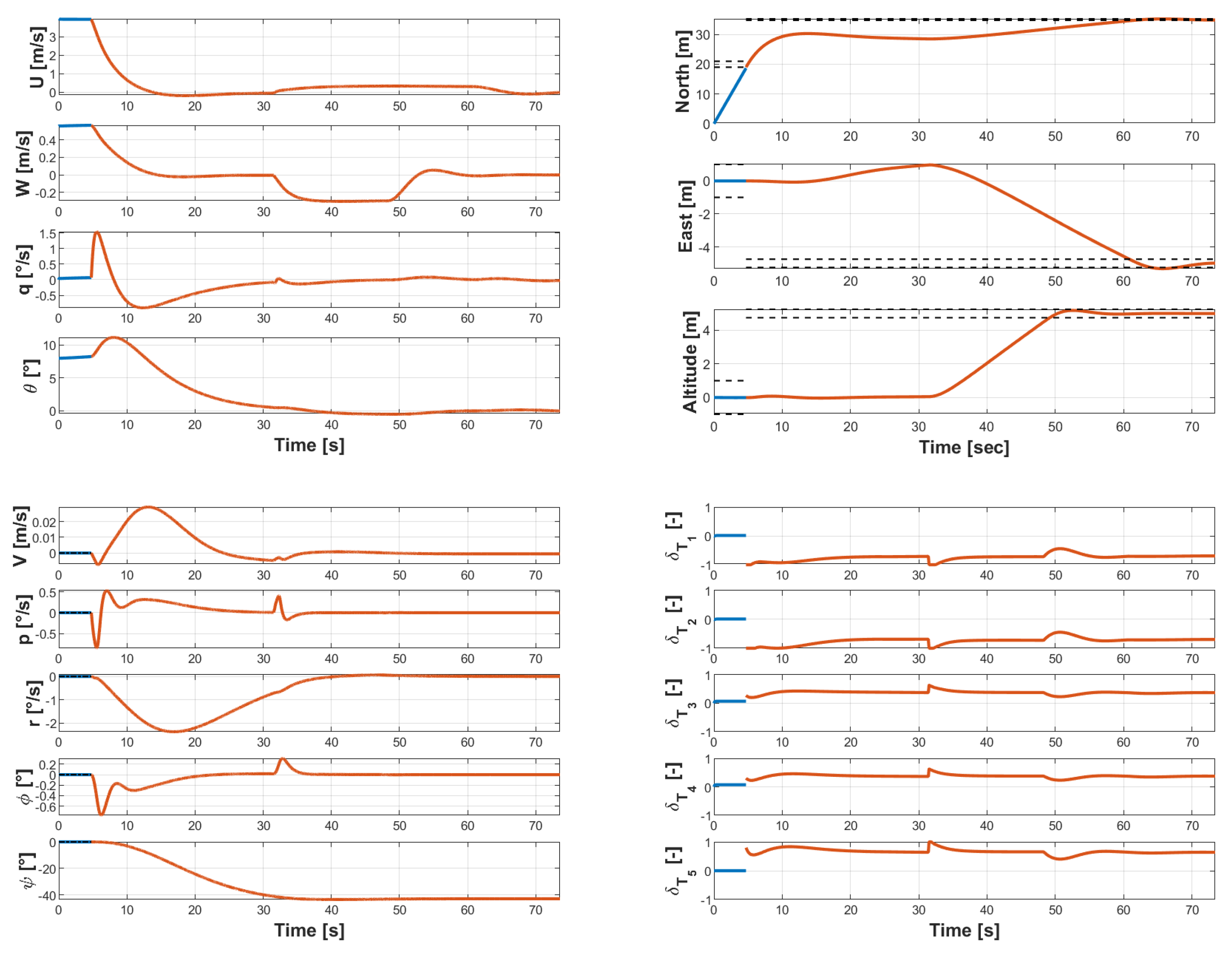
5.2.3. From forward Flight to Hover at Assigned Position-Longitudinal and Lateral-Directional Motion

In a last example, the same scenario presented in Section 5.2.2 is considered but the target point for hover is additionally displaced west (i.e., to the left of the airship traveling in forward flight to the north) by 5 m. The plots in Figure 9 portray the trajectory looking from the east (top-left), top (bottom-left) and from two different three-quarters attitudes (right). Similar to Figure 8, only the part of the trajectory corresponding to the HNHC mode on is shown (i.e., not the standard FFC navigation).

Upon engagement of the HNHC mode, according to the conceptual procedure in Section 4, the airship is controlled around the roll, pitch and yaw axes, to achieve the target deck angle ($\overline{\vartheta }=0$ deg) and aligning the longitudinal plane with the target vector $\mathit{d}$, thus reducing $|\psi - \overline{\psi }|$. At the same time, translation is damped, acting through $\Delta F_{HF}$ and $\Delta F_V$ to reduce speed, without momentarily requiring a repositioning in space. According to Equation (14), the alignment of the airship to point the target is carried out mostly imposing a moment $\Delta M_V$ in the ground horizontal plane, resulting primarily in an intense yaw motion. However, as explained in Section 4.2, a $\Delta F_{HL}^{{}^{\prime }}$ proportional to body lateral speed is also imposed, through a mild body-vertical thrust component and a concurrent minimal alteration of the roll angle, in turns achieved through $\Delta M_x$. Looking at the time history of longitudinal and lateral directional states (top- and bottom-left plots in Figure 10), it is apparent that lateral speed V, roll attitude $\phi$ and roll rate p take residual values, compared to the yaw rate r and yaw attitude $\psi$ (the latter is adjusted to obtain alignment with the target, yielding a rotation of around 40 deg to the left in the process). Similarly, on the bottom-right plot of Figure 10, the corresponding control action is generally mild (compare this result to the bottom-right plot in Figure 8, corresponding to the purely longitudinal near-hover navigation case).

Upon entering an alignment threshold of $\Delta {\psi }_{max}=3$ deg around the beam $\mathit{d}$ (happening around $t=32$ s in the simulation), the near-hover repositioning of the airship to the target point is started. In this part, the case under analysis is qualitatively equivalent to the one presented in Section 5.2.2. The top-left and top-right plots in Figure 10 show the behavior of the longitudinal states of the airship, and the components of the trajectory in the ground reference $\mathcal{I}$. The same strict requirement as in the previous test case is adopted for target reaching, represented by the horizontal dashed lines on the top-right plot of Figure 10.

The performance of the HNHC mode is fully explored in this case, showing the ability of the controller to carry out a near-hover navigation task in a three-dimensional scenario.

It should be noted that the directional control on $\psi$ is inhibited when nearing the target set for hover, so as to avoid divergence of the control demand, which would be encountered for an even slight inaccuracy in the lateral alignment when coming close to the target. This inhibition is typical when working with a radial angle measure (a common issue for instance in VOR-to-VOR autonomous air navigation). The threshold value of the three-dimensional radial distance from the target is $d_{min}=5$ m, under which $k_{\psi }$ in Equation (14) is set to zero, and $\Delta M_V$ is employed for damping only. It can be observed from the top-right plot of Figure 10 that the controller is generally effective in lateral control, achieving good accuracy in repositioning on the target in a limited time.

6. Conclusions

In this work, the problems of autonomous navigation in near-hover and of flight in hover at an assigned three-dimensional position have been investigated, for an unmanned thrust-controlled airship with no thrust vector control.

6.1. Proposed Control Strategy

A model-based control strategy with two logical layers has been described, implemented and tested.

6.1.1. First Control Layer: Static Equilibrium in Hover

In a first layer, the thrust demand for granting hover is computed. A formulation of static equilibrium has been introduced, highlighting the need for an arrangement of the thrusters on board such as to satisfy certain geometrical placement constraints. These constraints are analytically captured by the model and correspond to the well-posedness of the system of balance equations for equilibrium.

The outcome of this first control layer is the value of the thrust forces needed for static equilibrium in hover, which allow the airship to be kept in hovering flight at an assigned deck angle, even in the presence of a longitudinal displacement of the center of gravity with respect to the center of buoyancy. This largely overcomes the limitation of standard, aerodynamically controlled airships, which are basically incapable of hovering flight at a user-assigned deck angle.

Furthermore, the solution of the system for equilibrium comes in closed form for an assigned layout of the thrusters on board, yielding an easy adoption of the control algorithm in a realistic controller to employ in the field.

6.1.2. Second Control Layer: Stabilization and Navigation in Near-Hover

In a second layer, the proposed controller computes the thrust required to obtain steering actions from the thrusters in near-hover, based on the hypothesis of a negligible aerodynamic contribution to the forcing terms in the equations of motion of the airship.

Again, the computation of required thrust from a required system of steering forces and moments is obtained through a model, based on balance equations. This can be inverted yielding a closed-form solution in terms of thrust forces for an assigned layout of the thrusters on board.

Steering forces are computed based on standard proportional laws, closing loops on the rotational rates for stability augmentation, and on the relative position with respect to the target for navigation and station keeping. An assigned angle of the deck can be achieved in near-hover, similar to hover.

6.1.3. Overall Control Algorithm: Hover and Near-Hover Flight Control Mode

A control mode for near-hover and hover (HNHC mode) has been introduced, making use of thrust components obtained through the double-layer approach just mentioned. This complements the forward flight control mode (FFC) introduced by the authors in Ref. [16], yielding a complete suite for stabilization and navigation of a thrust-controlled airship with no thrust vector control.

6.2. Case Study

As a case study, in this paper a four-thruster, thrust-controlled autonomously flying airship concept has been considered, taken from previous studies and modified with the addition of a fixed, vertically pulling tail thruster intended for use in near-hover and hover. The proposed layout has been employed to apply the theoretical formulation for a thrust demand solution in hover and similarly thrust demands for a required steering action.

As pointed out, the considered five-thruster layout allows well-posed systems to be obtained for the tasks, thus yielding closed-form solutions in terms of thrust requirements from each thruster for hover and steering, which can be implemented in a controller online. Required data for the computation of thrust demands are limited to the geometrical layout of the thrusters (position on board and alignment), and basic data of the airship (mass, volume, density of air at hovering altitude and position of the center of gravity from the buoyancy center).

The general performance of the HNHC mode has been assessed in three examples of increasing complexity.

Transition to hover from a condition of forward flight, with no requirement on the target position, has been analyzed first, showing the ability of the controller for hover to keep the airship under control during a slow-down maneuver and to achieve a hovering flight condition, coping with a requirement on the target deck angle. Then, the ability to transition from forward flight to a station keeping condition (i.e., hover) has been evaluated, at first in a purely longitudinal case, then in a completely three-dimensional case, additionally requiring a re-alignment of the airship, by changing its track angle in slow-speed navigation, as well as its yaw angle.

The performance of the HNHC mode in this test case is deemed practically reasonable, with good stability of all state signals, limited target overshoots and good accuracy achieved in on-target positioning within a reasonable transient time. This is obtained with a limited number of control tuning parameters required from the mission planner.

This allows the present controller to be set as a baseline for thrust-controlled airships with no thrust vectoring, allowing further investigations and comparisons with future proposed control solutions.

6.3. Outlook

As an outlook, the sensitivity of the controller with respect to model uncertainties will need a dedicated assessment. Similarly, autonomous mission planning, i.e., the automatic definition of the target points to be flown via the proposed control and guidance law, will be the topic of future investigation, starting from previous experience by the authors in helicopter practice [33].

Concurrently, further investigation will be aimed at the analysis of a mixed flight control mode for managing station keeping in windy conditions. Actually, a condition of station keeping in an airstream is significantly more similar to a forward flight problem than a hovering problem in terms of dynamics (i.e., aerodynamics will be not negligible in general). For this reason, wind was not considered in the present study. However, station keeping may employ a three-dimensional fixed target point tracking logic, with some similarity to the approach presented herein. This mission type and the corresponding control mode may be the subject of a further study.

References

1. Elfes, A.; Bueno, S.; Bergerman, M.; Ramos, J. A semi-autonomous robotic airship for environmental monitoring missions. In Proceedings of the 1998 IEEE International Conference on Robotics and Automation (Cat. No. 98CH36146), Leuven, Belgium, 20 May 1998; Volume 4, pp. 3449–3455. [Google Scholar]
2. Jon, J.; Koska, B.; Pospíšil, J. Autonomous airship equipped with multi-sensor mapping platform. ISPRS-Int. Arch. Photogramm. Remote Sens. Spat. Inf. Sci. XL-5 W 2013, 1, 119–124. [Google Scholar] [CrossRef]
3. Fedorenko, R.; Krukhmalev, V. Indoor autonomous airship control and navigation system. In MATEC Web of Conferences; EDP Sciences: Evry, France, 2016; Volume 42, p. 01006. [Google Scholar]
4. Chu, A.; Blackmore, M.; Oholendt, R.G.; Welch, J.V.; Baird, G.; Cadogan, D.P.; Scarborough, S.E. A Novel Concept for Stratospheric Communications and Surveillance: Star Light. In Proceedings of the AIAA Balloon Systems Conference, Williamsburg, VA, USA, 21–24 May 2007. [Google Scholar] [CrossRef]
5. Smith, I.; Lee, M.; Fortneberry, M.; Judy, R. HiSentinel80: Flight of a high altitude airship. In Proceedings of the 11th AIAA Aviation Technology, Integration, and Operations (ATIO) Conference, Including the AIAA Balloon Systems Conference and 19th AIAA Lighter-Than, Virginia Beach, VA, USA, 20–22 September 2011; p. 6973. [Google Scholar]
6. Miller, S.H.; Fesen, R.; Hillenbrand, L.; Rhodes, J.; Baird, G.; Blake, G.; Booth, J.; Carlile, D.E.; Duren, R.; Edworthy, F.G. Airships: A New Horizon for Science. Technical report. arXiv 2014, arXiv:1402.6706. [Google Scholar]
7. Riboldi, C.E.D.; Rolando, A.; Regazzoni, G. On the feasibility of a launcher-deployable high-altitude airship: Effects of design constraints in an optimal sizing framework. Aerospace 2022, 9, 210. [Google Scholar] [CrossRef]
8. Young, M.; Keith, S.; Pancotti, A. An overview of advanced concepts for near space systems. In Proceedings of the 45th AIAA/ASME/SAE/ASEE Joint Propulsion Conference & Exhibit, Denver, CO, USA, 2–5 August 2009; p. 4805. [Google Scholar]
9. Manikandan, M.; Pant, R.S. Research and advancements in hybrid airships—A review. Prog. Aerosp. Sci. 2021, 127, 100741. [Google Scholar]
10. Carichner, G.E.; Nicolai, L.M. Fundamentals of Aircraft and Airship Design; AIAA Education Series; American Institute of Aeronautics and Astronautics, Inc.: Reston, VA, USA, 2013. [Google Scholar]
11. Kämpf, B. Flugmechanik und Flugregelung von Luftschiffen. Ph.D. Thesis, University of Stuttgart, Stuttgart, Germany, 2004. [Google Scholar] [CrossRef]
12. Kornienko, A. System Identification Approach for Determining Flight Dynamical Characteristics of an Airship from Flight Data. Ph.D. Thesis, University of Stuttgart, Stuttgart, Germany, 2006. [Google Scholar] [CrossRef]
13. Cai, Z.L. Research on Dynamical Modeling and Nonlinear Control of a Stratospheric Airship. Ph.D. Thesis, Shanghai JIAO TONG University, Shanghai, China, 2006. [Google Scholar]
14. Li, Y.; Nahon, M.; Sharf, I. Dynamics modeling and simulation of flexible airships. AIAA J. 2009, 47, 592–605. [Google Scholar] [CrossRef]
15. Yang, Y.; Wu, J.; Zheng, W. Design, modeling and control for a stratospheric telecommunication platform. Acta Astronaut. 2012, 80, 181–189. [Google Scholar] [CrossRef]
16. Riboldi, C.E.D.; Rolando, A. Thrust-Based Stabilization and Guidance for Airships without Thrust-Vectoring. Aerospace 2023, 10, 344. [Google Scholar] [CrossRef]
17. Beji, L.; Abichou, A. Tracking control of trim trajectories of a blimp for ascent and descent flight manoeuvres. Int. J. Control 2005, 78, 706–719. [Google Scholar] [CrossRef]
18. Cai, Z.; Qu, W.; Xi, Y.; Wang, Y. Stabilization of an underactuated bottom-heavy airship via interconnection and damping assignment. Int. J. Robust Nonlinear Control 2007, 17, 1690–1715. [Google Scholar] [CrossRef]
19. Sangjong, L.; Haechang, L.; Daeyeon, W.; Hyochoong, B. Backstepping approach of trajectory tracking control for the mid-altitude unmanned airship. In Proceedings of the AIAA Guidance, Navigation and Control Conference and Exhibit, Hilton Head, SC, USA, 20–23 August 2007; p. 6319. [Google Scholar]
20. Paiva, E.; Benjovengo, F.; Bueno, S.; Ferreira, P. Sliding mode control approaches for an autonomous unmanned airship. In Proceedings of the 18th AIAA Lighter-Than-Air Systems Technology Conference, Seattle, WA, USA, 4–7 May 2009. [Google Scholar]
21. Liesk, T.; Nahon, M.; Boulet, B. Design and experimental validation of a nonlinear low-level controller for an unmanned fin-less airship. IEEE Trans. Control Syst. Technol. 2013, 21, 149–161. [Google Scholar] [CrossRef]
22. Nagabhushan, B.L.; Tomlinson, N.P. Dynamics and control of a heavy lift airship hovering in a turbulent cross wind. J. Aircr. 1982, 19, 826–830. [Google Scholar] [CrossRef]
23. Nagabhushan, B.L.; Tomlinson, N.P. Thrust-vectored takeoff, landing, and ground handling of an airship. J. Aircr. 1986, 23, 250–256. [Google Scholar] [CrossRef]
24. Azinheira, J.R.; Moutinho, A.; De Paiva, E.C. Airship hover stabilization using a backstepping control approach. J. Guid. Control Dyn. 2006, 29, 903–914. [Google Scholar] [CrossRef]
25. Yang, Y.; Wu, J.; Zheng, W. Station-keeping control for a stratospheric airship platform via fuzzy adaptive backstepping approach. Adv. Space Res. 2013, 51, 1157–1167. [Google Scholar] [CrossRef]
26. Yang, Y.; Wu, J.; Zheng, W. Positioning control for an autonomous airship. J. Aircr. 2016, 53, 1638–1646. [Google Scholar] [CrossRef]
27. Riboldi, C.E.D.; Rolando, A. Layout Analysis and Optimization of Airships with Thrust-Based Stability Augmentation. Aerospace 2022, 9, 393. [Google Scholar] [CrossRef]
28. Pamadi, B.N. Performance, Stability, Dynamics, and Control of Airplanes; AIAA Education Series; American Institute of Aeronautics and Astronautics, Inc.: New York, NY, USA, 2004. [Google Scholar]
29. Munk, M.M. The Aerodynamic Forces on Airship Hulls; Technical Report; Report No. 184; National Advisory Committee for Aeronautics (NACA): Washington, DC, USA, 1926. [Google Scholar]
30. Lamb, H. Hydrodynamics; Dover Publications: New York, NY, USA, 1945. [Google Scholar]
31. Jones, S.P.; DeLaurier, J.D. Aerodynamic estimation techniques for aerostats and airships. J. Aircr. 1982, 20, 120–126. [Google Scholar] [CrossRef]
32. Mueller, J.; Paluszek, M.; Zhao, Y. Development of an aerodynamic model and control law design for a high altitude airship. In Proceedings of the AIAA 3rd “Unmanned Unlimited” Technical Conference, Workshop and Exhibit, Chicago, IL, USA, 20–23 September 2004; p. 6479. [Google Scholar]
33. Trainelli, L.; Gennaretti, M.; Bernardini, G.; Rolando, A.; Riboldi, C.E.D.; Redaelli, M.; Riviello, L.; Scandroglio, A. Innovative helicopter in-flight noise monitoring systems enabled by rotor-state measurements. Noise Mapp. 2016, 3. [Google Scholar] [CrossRef]
Figure 1. Basic airship geometry for the study of the equations of motion.
Drones 07 00545 g001
Figure 2. Thruster position and attitude with respect to the airship body.
Drones 07 00545 g002
Figure 3. Definition of target control force and moment components. (Left) Force components. (Right) Moment components.
Drones 07 00545 g003
Figure 4. Definition of feed-back signals for control. (Left) Heading control. (Right) Position control.
Drones 07 00545 g004
Figure 5. Schematic flowchart of proposed control system.
Drones 07 00545 g005
Figure 6. Views of the considered airship test-bed. (Left) Three-quarters view. (Right) View from left side.
Drones 07 00545 g006
Figure 7. Airship slowing down and reaching a hovering condition starting from a cruise in forward flight. No assigned target position in hover. (Top-left) Trajectory view from right-hand side of airship. (Bottom-left) Three-quarters view of the trajectory. (Top-right) Time histories of longitudinal states. (Bottom-right) Time histories of controls. Blue time histories: flight controlled via FFC mode. Red time histories: flight controlled via HNHC mode.
Drones 07 00545 g007
Figure 8. Airship navigating in near-hovering condition (piloted in HNHC mode) to a target point for hover. Purely longitudinal problem. (Top-left) Trajectory view from right-hand side of airship. (Bottom-left) Displacement with respect to north and altitude in inertial frame I . (Top-right) Time histories of longitudinal body states. (Bottom-right) Time histories of controls. Blue time histories: flight controlled via FFC mode. Red time histories: flight controlled via HNHC mode.
Drones 07 00545 g008
Figure 9. Trajectory views of airship navigating in near-hovering condition (piloted in HNHC mode) to a target point for hover, in a complete three-dimensional assigned station keeping case (longitudinal and lateral directional). (Top-left) Trajectory view looking from the east. (Bottom-left) Trajectory view from top. (Top-right) Three-quarters view from the southwest. (Bottom-right) Three-quarters view from the southeast.
Drones 07 00545 g009
Figure 10. Time histories corresponding to the case portrayed in Figure 9. (Top-left) Longitudinal body states. (Bottom-left) Lateral-directional body states. (Top-right) Components of trajectory in ground frame I . (Bottom-right) Controls. Blue time histories: flight controlled via FFC mode. Red time histories: flight controlled via HNHC mode.
Drones 07 00545 g010