Differentiator- and Observer-Based Feedback Linearized Advanced Nonlinear Control Strategies for an Unmanned Aerial Vehicle System

Abstract

This paper presents novel chattering-free robust control strategies for addressing disturbances and uncertainties in a two-degree-of-freedom (2-DOF) unmanned aerial vehicle (UAV) dynamic model, with a focus on the highly nonlinear and strongly coupled nature of the system. The novelty lies in the development of sliding mode control (SMC), integral sliding mode control (ISMC), and terminal sliding mode control (TSMC) laws specifically tailored for the twin-rotor MIMO system (TRMS). These strategies are validated through both simulation and real-time experiments. A key contribution is the introduction of a uniform robust exact differentiator (URED) to recover rotor speed and missing derivatives, combined with a nonlinear state feedback observer to improve system observability. A feedback linearization approach, using lie derivatives and diffeomorphism principles, is employed to decouple the system into horizontal and vertical subsystems. Comparative analysis of the transient performance of the proposed controllers, with respect to metrics such as settling time, overshoot, rise time, and steady-state errors, is provided. The ISMC method, in particular, effectively mitigates the chattering issue prevalent in traditional SMC, improving both system performance and actuator longevity. Experimental results on the TRMS demonstrate the superior tracking performance and robustness of the proposed control laws in the presence of nonlinearities, uncertainties, and external disturbances. This research contributes a comprehensive control design framework with proven real-time implementation, offering significant advancements over existing methodologies.

1. Introduction

Recently, UAVs have attracted the attention of researchers owing to their highly nonlinear, complex nature, and vast area of application. The TRMS model provides a beneficial platform for analyzing and developing control algorithms for UAV during crucial maneuvers. TRMS is a laboratory setup and an experimental prototype of a UAV system that resembles the flight of a helicopter model. It consists of two main rotors attached to the beam and is driven by two independent DC motors. The beam is counterbalanced using an arm with attached weights at its endpoint. The system has two DOF, through which it freely moves in the horizontal and vertical directions [1]. UAVs have many advantages such as compact size, flexible flight, vertical and horizontal takeoff, low cost, and adaptable features. Therefore, TRMS can be used in real-time practical experiments of UAVs and has many applications for executing complex tasks, such as aircraft control, autonomous vehicles, robotic manipulation, and industrial automation [2].

It is a formidable challenge to control the pitch and yaw angles of the UAV due to the inherited coupling effects and extreme nonlinearities in the system dynamics. Various researchers across the globe have been tackling these challenges by developing precise dynamic models and robust control techniques for system stability. This study is dedicated to the design of advanced UAV control strategies through innovative and robust control laws and their real-time implementation to validate their performance. The main focus is to enhance both robustness and tracking performance in the presence of uncertainties and disturbances. The following paragraphs delve into the array of methodologies that have been adopted and refined by the researchers in recent years, highlighting their contributions and advancements.

A genetic algorithm (GA)-based proportional integral derivative (PID) control was designed to tackle the complexities of nonlinear dynamic models, aiming to reduce modeling errors and improve convergence. Despite these intentions, the method fell short due to fixed system parameters, resulting in less effective performance [3]. In contrast, SMC and higher-order SMC (HOSMC) controllers with state varying gain (VG) were applied to a two-DOF dynamic model. Unfortunately, these algorithms struggled with unsatisfactory transient performance, chattering issues, and lacked validation through real-time experimentation [4]. Integral back-stepping (BS) and super-twisting algorithms using bond graphs have been proposed for real-time testing. Integral BS enhances the slow pitch and yaw movement, whereas the super-twisting scheme controls the fast actuator dynamics [5]. The robust generalized inversion-based (RGIB) technique presented in [6] introduces a novel approach to addressing the challenges of coupling effects and singularity issues in control system design. By establishing a feedback linearized platform, this method aims to mitigate the complexities associated with these phenomena. Through its robust generalized inversion-based framework, the RGIB offers a systematic strategy for effectively handling the intricate interplay between system dynamics and control actions, thereby enhancing the stability and performance of the overall control system. SMC and HOSMC algorithms, combined with input–output feedback linearization techniques, were implemented for a highly coupled system in the presence of model uncertainties and disturbances to decompose it into linear sub-system. Since the relative degree of the system is less than its order, i.e., $r < n$, a feedback linearization technique was employed to control the outputs of the coupled system, ensuring closed-loop stability and fast dynamic convergence of the system state variables [7].

A discrete feedback linearization approach is implemented to control the yaw movement of an unmanned helicopter model. However, despite the proposed method, it is observed that the approach remains highly sensitive to noise factors, consequently leading to degradation in system performance [8]. A new RGI sliding surface has been proposed using SMC to control the pitch and yaw orientation movement, but the cross-coupling effect degrades the system performance during precise measurement; thus, movement along with the freedom to operate the system in a nonlinear range is not achieved [9]. A synthesized SMC with disturbance-observer-based control is successfully tested through simulations and verified for a UAV [10]. A robust H-infinity (∞)-based controller is proposed in [11]. However, the standard linear H(∞) controller synthesized by the loop design procedure (LSDP) offers robustness at the cost of performance to overcome the cross-coupling effect and eliminate it by considering it an external perturbation and utilizing the feedback linearization approach. The H-infinity (∞) control theory in [12] defines the conditions for local disturbance attenuation with internal stability with measurement feedback. This feedback linearization setup is crucial for robust performance in nonlinear affine systems. The study demonstrates that disturbance attenuation retains a meaningful frequency-domain interpretation even in nonlinear setups. It also establishes a family of controllers that ensure robustness for both linear and nonlinear systems using dissipation inequality and LaSalle’s invariance principle. Thus, clear conditions for controller design are essential for stability and disturbance rejection, emphasizing the need for a thorough understanding of feedback linearization techniques in various contexts.

An adaptive fuzzy control scheme is developed for guidance and control to reduce errors and control the input energy of the system. The obtained simulation results depict chattering in the SMC law, whereas the overall system exhibits smooth and robust tracking performance [13]. In [14], integrator BS and an adaptive estimator through feedback control are developed to control azimuth and pitch angle movement in the presence of parametric uncertainties. The convergence is verified through simulation and experimental results within a specified time constraint. A disturbance-observer-based model predictive control design is developed and tested with mapped input–output constraints to handle external disturbances; however, this technique does not incorporate asymptotically to minimize uncertainties and for the application of feedback regulation [15]. SMC and TSMC are used for small UAVs by considering the system dynamic model in two single-input single-output (SISO) subsystems. Thus, the nonlinear surface used for the TSMC law provides faster and finite-time convergence and makes the system more robust. SMC and TSMC are compared to achieve better control performance, but the convergence time and chattering problem are not effectively improved through the proposed control strategies [16]. However, a decoupling technique has not been implemented, leading to increased control effort.

An integral SMC for small helicopters is proposed to minimize the adverse effects of disturbances. Stability is achieved through an approximated input–output feedback control approach and Lyapunov stability theorem and then verified for convergence and tracking errors [17,18]. Additionally, a novel ISMC is designed for the relative degree goal to reject external perturbations. However, owing to the improper design of the sliding surface, the system becomes more complex, and the tracking problem of output trajectories arises. Thus, the controller obtained is not feasible for stable and long smooth flights [19]. A non-singular TSMC is proposed in [20] for chattering attenuation and finite-time convergence in small helicopters. The obtained simulation-based results are insufficient because no real-time testing is considered to analyze the mismatched disturbance, resulting in more overshoot and steady-state error. Moreover, a MIMO system is decomposed into an SISO system and controlled through TSMC for a small, unmanned helicopter. A closed-loop analysis of the system indicates that the control performance depends entirely on the initially adjusted control parameters and does not rely on the initial set state values [21].

Observers can be readily designed for nonlinear systems that can be transformed into a linear form through a change in state variables and output injection. The necessary and sufficient conditions for the existence of such a transformation are provided [22].

Unlike previous studies that primarily focus on simulation, this research extends the control strategies to real-time experiments, validating their applicability and robustness. SMC provides robust control but suffers from chattering, which is mitigated by ISMC. TSMC, with its finite-time convergence, improves system response time. The decoupling of the system into horizontal and vertical subsystems using feedback linearization further enhances the control design, allowing for independent subsystem regulation. Through a detailed comparison of SMC, ISMC, and TSMC, this paper offers an in-depth analysis of their respective strengths and weaknesses, demonstrating that ISMC provides the best trade-off between performance and chattering reduction.

The contributions of this research are summarized as follows:

• Development and experimental validation of SMC, ISMC, and TSMC for the TRMS, with ISMC offering significant improvements in chattering reduction and system robustness;
• Application of feedback linearization to decouple the UAV system into horizontal and vertical subsystems for better control accuracy and stability;
• Integration of a URED for enhanced differentiation in the presence of system uncertainties and disturbances.

The remainder of this paper is organized as follows: Section 2 describes the nonlinear decoupled mathematical dynamic model based on input–output feedback linearization for TRMS. Section 3 discusses the control design of SMC, ISMC, TSMC and URED, and state feedback observer design is explicitly carried out along with stability analysis using Lyapunov stability criteria. Section 4 presents the numerical simulation and experimental results obtained, along with the effectiveness and validity of the simulated and experimental tested test results. Transient and quantitative performance analyses are presented in this section to compare the results obtained in the simulation and experiments on a physical TRMS. Finally, Section 5 concludes the paper.

As the literature involves the use of a lot of acronyms,

Table 1. Acronyms and definition.

Acronyms	Definition
MIMO	Multiple Input Multiple Output
TRMS	Twin Rotor MIMO System
SMC	Sliding Mode Control
HOSMC	Higher Order Sliding Mode Control
DC	Direct Current
TSMC	Terminal Sliding Mode Control
UAV	Unmanned Aerial Vehicle
SISO	Single Input Single Output
RGIB	Robust Generalized Inversion-Based
PID	Proportional Integral Derivative
LQR	Linear Quadratic Regulator
DOF	Degree Of Freedom
GA	Genetic Algorithm
VG	Variable Gain

defines them.

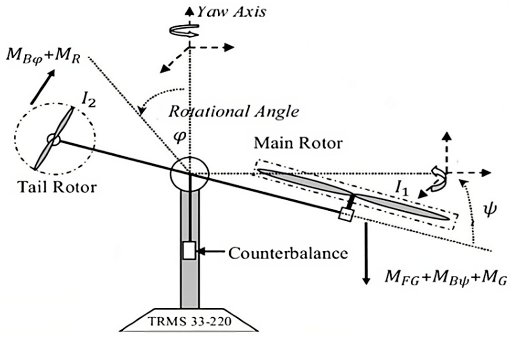
2. Mathematical Nonlinear Model

TRMS is a MIMO system that is mainly used for real-time testing of design control algorithms. The laboratory prototype setup of this system is designed and developed by Feedback Limited Company, as shown in Figure 1. It is an electromechanical system comprising separate mechanical and electrical units. The mechanical part consists of main and tail motors. Each motor is driven independently by an individual DC motor, and both rotors are counterbalanced through the attached beam, which provides additional stability to the system. The main and tail motor blades produce a thrusting force that removes the system in vertical and horizontal directions [23]. By maintaining the angle of attack constant, we can change the thrust force based on the speed of the motors.

The dynamic model of the TRMS is obtained using Newton’s second-law approach. According to the law of conservation, motors experience a thrust force opposite to that of accelerated air. The two motors are perpendicular to the plane and exhibit strong coupling effects [24].

Table 2. Assigned parameter values for the TRMS model.

Parameters	Definition	Value	Unit
$I_1$	Moment of inertia for vertical rotor	6.7 × ${10}^{-2}$	$\mathrm{K}\mathrm{g}.{\mathrm{m}}^2$
$I_2$	Moment of inertia for horizontal rotor	2.1 × ${10}^{-2}$	$\mathrm{K}\mathrm{g}.{\mathrm{m}}^2$
$a_1$	Static characteristics parameter	0.0	-
$a_2$	Static characteristics parameter	0.03	-
$b_1$	Static characteristics parameter	0.09	-
$b_2$	Static characteristics parameter	0.092	-
$M_g$	Gyroscopic momentum	0.5	$\mathrm{N}.\mathrm{m}$
$B_{1\psi }$	Frictional momentum	6 × ${10}^{-4}$	$\mathrm{N}.\mathrm{m}.\mathrm{s}/\mathrm{r}\mathrm{a}\mathrm{d}$
$B_{2\psi }$	Frictional momentum	1 × ${10}^{-2}$	$\mathrm{N}.\mathrm{m}.{\mathrm{s}}^2/\mathrm{r}\mathrm{a}\mathrm{d}$
$B_{1\phi }$	Frictional momentum	1 × ${10}^{-3}$	$\mathrm{N}.\mathrm{m}.\mathrm{s}/\mathrm{r}\mathrm{a}\mathrm{d}$
$B_{2\phi }$	Frictional momentum	1 × ${10}^{-2}$	$\mathrm{N}.\mathrm{m}.{\mathrm{s}}^2/\mathrm{r}\mathrm{a}\mathrm{d}$
$K_{gy}$	Gyroscopic momentum	0.04	$\mathrm{s}/\mathrm{r}\mathrm{a}\mathrm{d}$
$K_1$, $K_2$	Motor 1 and motor 2 gains	1.1, 2	-
$T_{11}{,T}_{10},T_{21},T_{20}$	Motor 1 and Motor 2 denominator parameters	2, 1, 1.5, 1	-
$T_{p,}{T}_{o,}{K}_c$	Cross reaction momentum parameters	2, 3, −0.5	-

presents a detailed comparison of the numerical performance of the designed controllers. The mathematical model for TRMS, along with the vertical and horizontal plans, is presented below:

The moment equation for the horizontal and vertical plan are given as

$$\begin{gathered} I_1\ddot{\psi }=M_1-M_{FG}-M_{B\psi }-M_g \\ {I}_2\ddot{\phi }=M_2-M_{B\phi }-M_R \end{gathered}$$

(1)

where the nonlinear static characteristics for the main motor are given by

$$M_1=a_1{\tau }_1^2+b_1{\tau }_1$$

(2)

The gravity moment and fractional force momentum is presented by

$$\begin{gathered} M_{FG}=M_g\sin \psi \\ {M}_{B\psi }=B_{1\psi }\dot{\psi }+B_{2\psi }\sin \dot{\psi } \end{gathered}$$

(3)

The gyroscopic momentum is considered as

$$M_g=K_{gy}{M}_1\dot{\phi }\cos \psi$$

(4)

The nonlinear static characteristics and friction force moment for the tail motor are presented as

$$\begin{gathered} M_2=a_2{\tau }_2^2+b_2{\tau }_2 \\ {M}_{B\psi }=B_{1\phi }\dot{\psi }+B_{2\phi }sign\left(\dot{\psi }\right) \end{gathered}$$

(5)

The cross-reaction moment can be written as

$$M_R={\displaystyle \frac{K_c\left(T_{0s}+1\right)}{(T_{p}s+1)}}{\tau }_1$$

(6)

The DC motor electrical circuit is approximated using a first-order transfer function in the Laplace domain. The momentum for both rotors is given as

$${\tau }_1={\displaystyle \frac{K_1}{(T_{11}s+T_{10})}}{u}_1$$

(7)

$${\tau }_2={\displaystyle \frac{K_2}{(T_{21}s+T_{20})}}{u}_2$$

(8)

The mathematical dynamic model of TRMS is presented with the following equations:

$${\displaystyle \frac{d\dot{\psi }}{dt}}={\displaystyle \frac{a_1}{I_1}}{{\tau }_1}^2+{\displaystyle \frac{b_1}{I_1}}{\tau }_1-{\displaystyle \frac{M_g}{I_1}}\sin \left(\psi \right)-{\displaystyle \frac{B_1\psi }{I_1}}\dot{\psi }+{\displaystyle \frac{0.0326}{2I_1}}\sin \left(2\psi \right){\dot{\psi }}^2-{\displaystyle \frac{K_{gy}}{I_1}}\cos \left(\psi \right)\phi (a_1{{\tau }_1}^2+b_1{\tau }_1)$$

$${\displaystyle \frac{d\dot{\phi }}{dt}}={\displaystyle \frac{a_2}{I_2}}{{\tau }_2}^2+{\displaystyle \frac{b_2}{I_2}}{\tau }_2-{\displaystyle \frac{B_{1\phi }}{I_2}}\dot{\phi }-{\displaystyle \frac{K_c}{I_2}}1.75(a_1{\dot{\phi }}^2+b_1\dot{\phi })$$

Here, all the variables in the above equation are in terms of $x$. Therefore, $x_1=\psi$, $x_2=\dot{\psi }$, $x_3=\phi$, $x_4=\dot{\phi }$, $x_5={\tau }_1$ and $x_6={\tau }_2$. The mathematical state space representation of coupled TRMS in term of $x$ can be presented as follows:

$$\left\{\begin{array}{c}{\dot{x}}_1=x_2\\ {\dot{x}}_2={\displaystyle \frac{a_1}{I_1}}{x}_5^2+{\displaystyle \frac{b_1}{I_1}}{x}_5-{\displaystyle \frac{M_g}{I_1}}\mathit{sin}\left(x_1\right)-{\displaystyle \frac{B_1{x}_1}{I_1}}{x}_2+{\displaystyle \frac{0.0236}{2I_1}}\mathit{sin}\left(2x_2\right)x_4^2-{\displaystyle \frac{K_{gy}}{I_1}}{a}_1\mathit{cos}\left(x_1\right)x_4{x}_5^2-\\ {\displaystyle \frac{K_{gy}}{I_1}}{b}_1\mathit{cos}\left(x_1\right)x_4{x}_5\\ {\dot{x}}_3=x_4\\ {\dot{x}}_4={\displaystyle \frac{a_2}{I_2}}{x}_6^2+{\displaystyle \frac{b_2}{I_2}}{x}_6-{\displaystyle \frac{B_1{x}_3}{I_2}}{x}_4-{\displaystyle \frac{K_c}{I_2}}{a}_{1}1.75x_5^2-{\displaystyle \frac{1.75}{I_2}}{K}_c{b}_1{x}_5\\ {\dot{x}}_5=-{\displaystyle \frac{T_{10}}{T_{11}}}{x}_5+{\displaystyle \frac{K_1}{T_{11}}}{u}_1\\ {\dot{x}}_6=-{\displaystyle \frac{T_{20}}{T_{21}}}{x}_6+{\displaystyle \frac{K_2}{T_{21}}}{u}_2\end{array}\right.$$

The system input vectors, state equation and control input in new coordinates can be presented as follows:

$$\left\{\begin{array}{c}Z={\left[Z_1,Z_2,Z_3,Z_4,Z_5,Z_6\right]}^T={\left[\psi ,\dot{\psi },\phi ,\dot{\phi ,}{\tau }_1,{\tau }_2\right]}^T\\ y={\left[\psi ,\phi \right]}^T\\ u={\left[u_1,u_2\right]}^T\end{array}\right.$$

Here, $Z_1$ and $Z_2$ represent the yaw angle and yaw angular velocity for the main rotor around the vertical axis, respectively. Where $Z_3$ and $Z_4$ denote the pitch angle and pitch angular velocity for the tail rotor around horizontal axis. Meanwhile, $Z_5$ and $Z_6$ correspond to the angular velocities of the main and tail rotor, respectively. Additionally, $\psi$ and $\dot{\psi }$ denote the position and velocity for the vertical plane, while $\phi$ and $\dot{\phi }$ represent the angle and angular velocity, respectively.

Assumption 1.

Using the input–output feedback linearization technique, the dynamics of the coupled TRMS are decoupled into horizontal and vertical subsystems by employing newly mapped coordinates, effectively achieving decoupling.

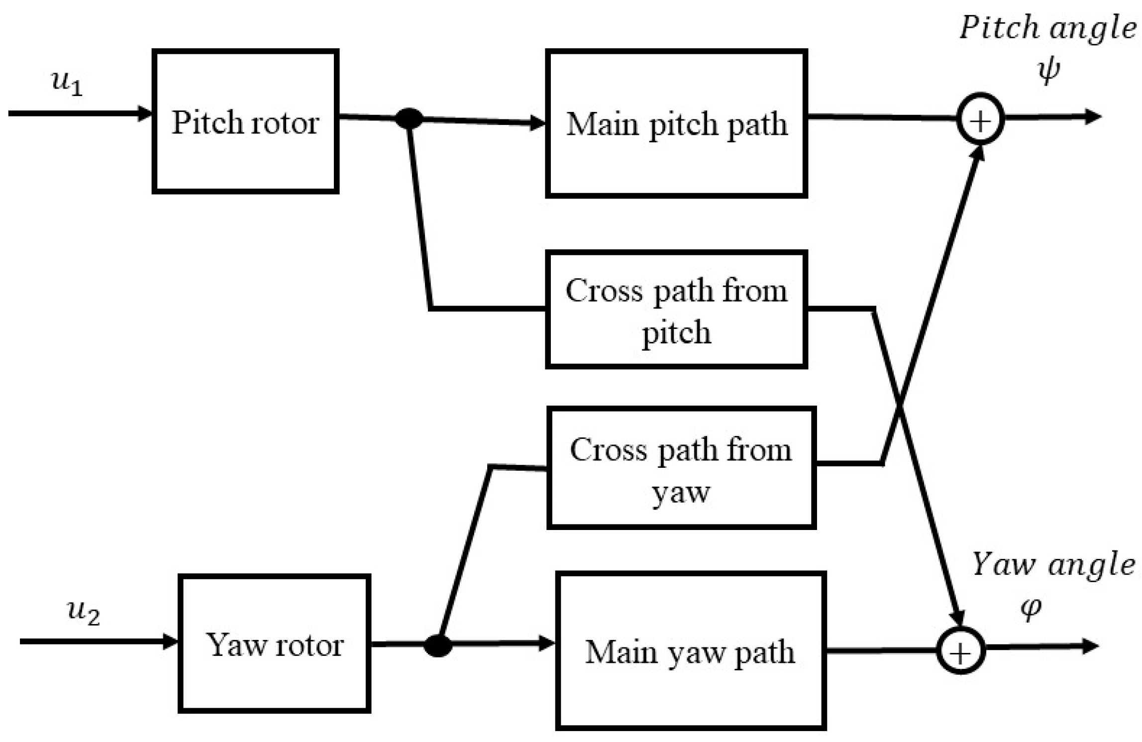
2.1. Feedback Linearization

This section illustrates the application of the input–output feedback linearization technique for highly coupled TRMS. Feedback linearization is a common approach employed to control the behavior of nonlinear systems. In our case, the relative degree of the system is $k=3$, and the system order is $n=6$, which is greater than the relative degree $n>k$; therefore, we used the input–output feedback linearization method to make the relative degree and system order equal. As shown in Figure 2, this approach aims to transform a highly nonlinear and coupled system into a linearized decoupled form through coordinate transformation. By employing an appropriate transformation function, nonlinear state variables can be converted into new linear state variables. This transformation alters the system variables, rendering the system more convenient for robust nonlinear control design. The general representation for the vector field and system output equations can be presented by

$$\begin{gathered} \dot{x}=f\left(x\right)+g\left(x\right)u \\ y=h\left(x\right) \end{gathered}$$

(9)

where $x \mathsf{ϵ}{ R}^n$ and $u \mathsf{ϵ} R^m$ represent the system states and control inputs while $h\left(x\right)$ and $g\left(x\right)$ are the vector fields. Generally, the state space representation for the state transformation can be given by

$$\psi \left(x\right),\phi \left(x\right)=\left[\begin{array}{c}{\psi }_1\left(x\right),{\phi }_1\left(x\right)\\ {\psi }_2\left(x\right), {\phi }_2\left(x\right) \\ {\psi }_{i-1}\left(x\right), {\phi }_{i-1}\left(x\right) \end{array}\right]=\left[\begin{array}{c}h\left(x\right)\\ L_{f}h\left(x\right)\\ L{f}^{i-1}h\left(x\right)\end{array}\right]$$

(10)

where the notations $L_{f}h\left(x\right)$ and ${L_f}^{2}h\left(x\right)$ are used for the lie derivative of function $h\left(x\right)$ along with the vector field $f\left(x\right)$ and $Z_i={\psi }_i\left(x\right),\phi \left(x\right)=L{f}^{i-1}h\left(x\right)$; $i⩽1⩽n$ and lie derivative of a function $h\left(x\right)$:${\mathbb{R}}^n$ → ℝ, with the vector field are given as

$$f\left(x\right)=f_1\left(x\right),\dots \dots \dots .,f_1\left(n\right)$$

where

$$\left\{\begin{array}{c}{L}_{f}h\left(x\right)={\displaystyle \sum _{i=n}^n}{\displaystyle \frac{\partial h}{\partial x_i}}{f}_i(x)\\ L^{i}fh=Lf\left(L{f}^{i-1}h\right)\end{array}\right.$$

The coordinate mapping state space representation for TRMS can then be presented by

$$\psi \left(x\right),\phi \left(x\right)=\left[\begin{array}{c}{\psi }_1\left(x\right),{\phi }_1\left(x\right)\\ {\psi }_2\left(x\right), {\phi }_2\left(x\right) \\ {\psi }_3\left(x\right), {\phi }_3\left(x\right) \end{array}\right]=\left[\begin{array}{c}h\left(x\right)\\ L_{f}h\left(x\right)\\ {L_f}^{2}h\left(x\right)\end{array}\right]=\left[\begin{array}{c}{\dot{Z}}_{1a}, {\dot{Z}}_{1b}\\ {\dot{Z}}_{2a}, {\dot{Z}}_{2b}\\ {\dot{Z}}_{3a}, {\dot{Z}}_{3b}\end{array}\right]$$

(11)

2.1.1. Vertical Decoupled Subsystem

Utilizing the lie derivative and by incorporating the previously mentioned notations, the newly mapped coordinates for the nonlinear decoupled vertical subsystem, based on Assumption 1, can be formulated into state space representation as

$$\begin{gathered} {\dot{Z}}_{1a}=Z_{2a} \\ {\dot{Z}}_{2a}={\displaystyle \frac{a_1}{I_1}}{Z}_{3a}^2+{\displaystyle \frac{b_1}{I_1}}{Z}_{3a}-{\displaystyle \frac{M_g}{I_1}}\sin \left(Z_{1a}\right)-{\displaystyle \frac{B_1\psi }{I_1}}{Z}_{2a} \\ {\dot{Z}}_{3a}=-{\displaystyle \frac{T_{10}}{T_{11}}}{Z}_{3a}+{\displaystyle \frac{K_1}{T_{11}}}{u}_1 \end{gathered}$$

(12)

where $[{\dot{Z}}_{1a},{\dot{Z}}_{2a},{\dot{Z}}_{3a}]=[\psi ,\dot{\psi },{\tau }_1]$ and $\psi , \dot{\psi }, \mathrm{a}\mathrm{n}\mathrm{d} {\tau }_1$ represent the pitch angle, angular velocity and torque of the main rotor, respectively.

2.1.2. Horizontal Decoupled Subsystem

The nonlinear decoupled subsystem, by considering Assumption 1, can be presented into state space form as follows:

$$\begin{gathered} {\dot{Z}}_{1b}=Z_{2b} \\ {\dot{Z}}_{2b}={\displaystyle \frac{a_2}{I_2}}{Z}_{3b}^2+{\displaystyle \frac{b_2}{I_2}}{Z}_{3b}-{\displaystyle \frac{B_{1\phi }}{I_2}}{Z}_{2b}-{\displaystyle \frac{K_c}{I_2}}{1.75(a}_1{Z}_{2b}^2+b_1{Z}_{2b}) \\ {\dot{Z}}_{3b}=-{\displaystyle \frac{T_{20}}{T_{21}}}{Z}_{3b}+{\displaystyle \frac{K_2}{T_{21}}}{u}_2 \end{gathered}$$

(13)

where [${\dot{Z}}_{1b},{\dot{Z}}_{2b},{\dot{Z}}_{3b}]=[\phi ,\dot{\phi ,}{\tau }_2]$ and $\phi ,\dot{ \phi ,}{ \tau }_2$ represent the yaw angle, angular velocity and torque for the tail rotor.

Remark 1.

The objective of this study is to design different robust controllers that efficiently track the desired system output pitch and yaw angle trajectories $(y_{1d}$, $y_{2d})$ in the presence of disturbances. For $t\succcurlyeq 0$, the disturbance $∆\left(t\right)$ along its derivative $\dot{∆}\left(t\right)$ is norm-bounded, i.e., $‖∆\left(t\right)‖ <{ N}_d$ and $‖\dot{∆}\left(t\right)‖ < \widehat{N_d},$ where $N_d$ represents the known positive constant and $\widehat{N_d}$ is an unknown positive constant.

Assumption 2.

For a closed-loop system, it is assumed that the dynamics of TRMS, including the pitch and yaw angle movements, are stable when using SMC, ISMC and TRMC laws. The designed robust control laws ensure the convergence of sliding mode behavior within finite time, even in the presence of system-bounded uncertainties. Consequently, the tracking errors are expected to converge to zero within a finite time frame.

Assumption 3.

It is assumed that the input state equations defined in the system mathematical model, along with the control inputs $u_1$ and $u_2$, are appropriately designed such that both the vertical and horizontal movements of twin rotor MIMO system achieve stability under the application of SMC, ISMC and TSMC strategies.

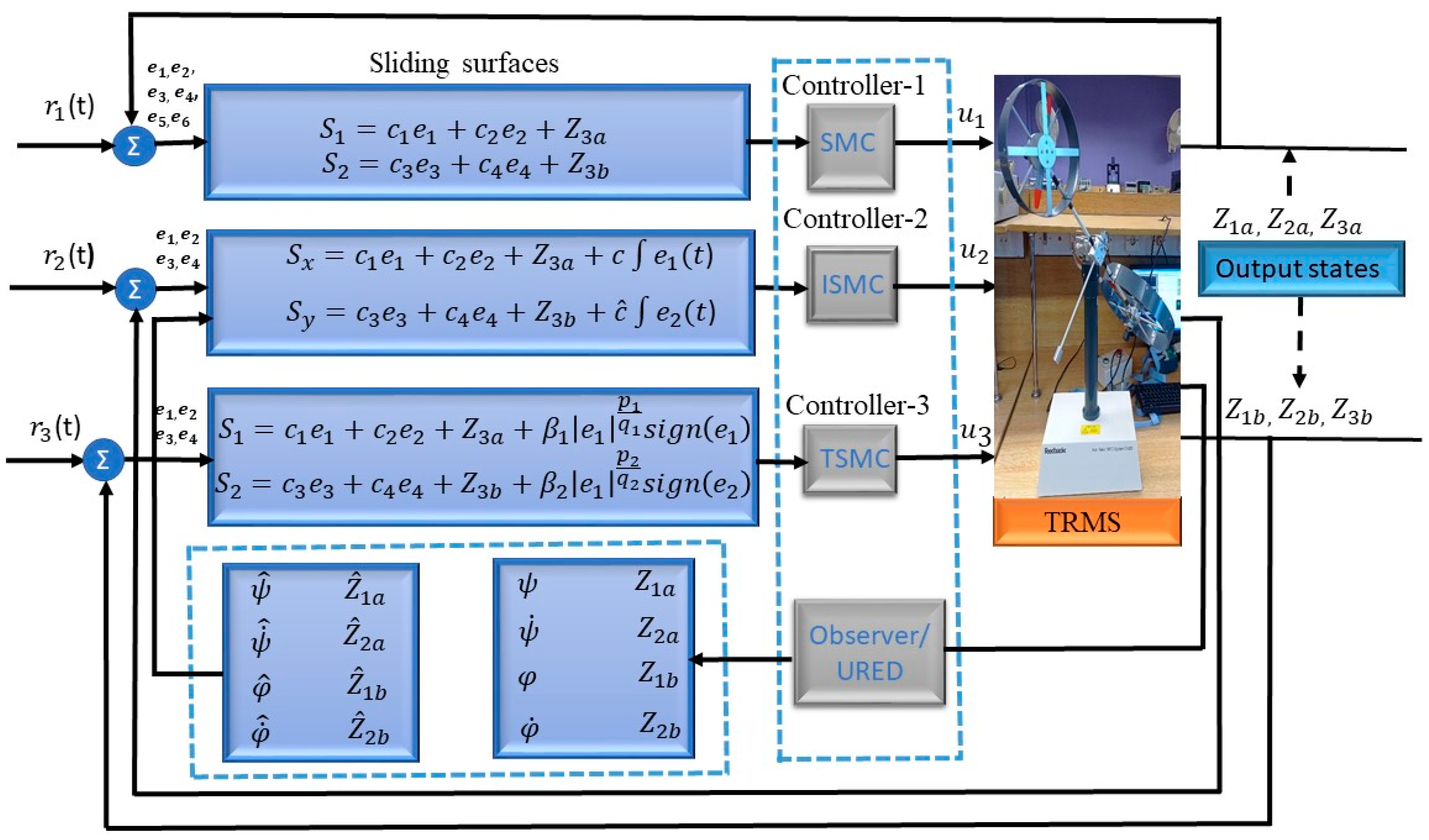
3. Robust Control Strategies

A TRMS is an actuated system with strong coupling effects between the rotors. Therefore, nonlinear robust control algorithms have been proposed to obtain desired results. This section presents the step-by-step control design of the SMC, ISMC, TSMC, URED, and state feedback observer for TRMS. The objective is to design various controllers and observers that can achieve robust autonomous performance against disturbances and uncertainties. The chattering that arises in the control input of the SMC law is consequently eliminated through the ISMC and TSMC laws, and both output angles show smooth flights in the horizontal and vertical directions, which also converge the system states to an equilibrium position within a finite time. The following subsection and Figure 3 present the designs of the SMC, ISMC, TSMC laws, URED, and state feedback observer.

3.1. Sliding Mode Control

SMC is a nonlinear robust control technique that is employed in complex dynamics and MIMO systems. This technique is based on the Lyapunov stability theorem and ensures the rejection of external disturbances present in the system. A drawback of the SMC law is the chattering effect. Therefore, the ISMC law is proposed in the next section to minimize this effect. SMC design mainly involves sliding and reaching phases [25]. In the reaching phase, the system moves into the sliding manifold through an equivalent controller, whereas in the reaching phase, the system states remain in equilibrium. The error dynamics for the controller are given by

$$\left\{\begin{array}{c}{e}_1={\phi }_1-{\phi }_{1d}\\ \dot{e_1}={\dot{\phi }}_1-{{\dot{\phi }}_1}_d\\ e_2={\phi }_2-{\phi }_{2d}\\ \dot{e_2}={\dot{\phi }}_2-{{\dot{\phi }}_2}_d\end{array}\right. \mathrm{and} \left\{\begin{array}{c} e_3={\psi }_3-{\psi }_{3d}\\ \dot{e_3}={\dot{\psi }}_3-{\dot{\psi }}_{3d}\\ e_4={\psi }_4-{\psi }_{4d}\\ \dot{e_4}={\dot{\psi }}_4-{\dot{\psi }}_{4d}\end{array}\right.$$

The sliding surface for the pitch angle are defined as

$$S_1=c_1{e}_1+c_2{e}_2+Z_{3a}$$

(14)

where $c_1$ and $c_2$ are the positive constant and tuning parameters while $e_1$ and $e_2$ represent the tracking errors. Taking the derivative of Equation (14) becomes

$$\dot{S_1}=c_1\dot{e_1}+c_2\dot{e_2}+{\dot{Z}}_{3a}$$

(15)

The SMC law incorporates two controller parts, i.e., equivalent control ($u_{1eq})$ and discontinuous control ${(u}_{1dis}).$ The equivalent controller part is obtained by considering the sliding surface with respect to time at $\dot{S_1}=0$. The equivalent controller part for the pitch angle is computed as follows:

$$u_{1eq}={\displaystyle \frac{-T_{11}}{K_1}}(c_1({\phi }_2-{\dot{\phi }}_{1d})+c_2(\dot{{\phi }_2}-{\dot{\phi }}_{2d})-{\displaystyle \frac{T_{10}}{T_{11}}}{Z}_{3a}$$

(16)

where switching control law is given by $u_{1dis}=-n_{1}Sign\left(S_1\right)$. Therefore, the overall control law for the pitch angle is computed as the sum of $u_{1eq}$ and $u_{1dis}$ as follows:

$$u_{1t}={\displaystyle \frac{-T_{11}}{K_1}}(c_1({\phi }_2-{\dot{\phi }}_{1d})+c_2(\dot{{\phi }_2}-{\dot{\phi }}_{2d})-{\displaystyle \frac{T_{10}}{T_{11}}}{Z}_{3a}-n_{1}Sign\left(S_1\right)$$

(17)

where the controller tuning parameters should be greater than zero, i.e., $c_1,c_2,n_1>0$. The sliding surface for the yaw angle is given as

$$S_2=c_3{e}_3+c_4{e}_4+Z_{3b}$$

(18)

The derivative of sliding surface $S_2$ can be written as

$$\dot{S_2}=c_3\dot{e_3}+c_4\dot{e_4}+{\dot{Z}}_{3b}$$

(19)

Now, when ${\dot{S}}_2=0$, the equivalent control for the yaw angle is considered as follows:

$$u_{2eq}={\displaystyle \frac{-T_{21}}{K_2}}{c}_3\left({\psi }_4-{\dot{\psi }}_{3d}\right)+c_4\left(\dot{{\psi }_4}-{\dot{\psi }}_{4d}\right)-{\displaystyle \frac{T_{20}}{T_{21}}}{Z}_{3b}$$

(20)

The reaching law is given by $u_{2dis}=-n_{2}Sign\left(S_2\right)$. The equivalent and switching control law for the yaw angle can be presented by

$$u_{2t}={\displaystyle \frac{-T_{21}}{K_2}}{c}_3\left({\omega }_y-{\dot{\psi }}_{3d}\right)+c_4\left(\dot{{\psi }_4}-{\dot{\psi }}_{4d}\right)-{\displaystyle \frac{T_{20}}{T_{21}}}{Z}_{3b}-n_{2}Sign\left(S_2\right)$$

(21)

where the tuning parameters $c_1$, $c_2$, $c_3$, $c_4$, $n_1$ and $n_2$ are the controller tuning parameters as given in

Table 3. Tuning parameters for the controllers.

Parameters	SMC	ISMC	TSMC	URED/Observer
$n_{1,}{n}_2$	5, 11	-	-	-
$c_{1,}{c}_2$	3.3, 7	4.8, 4	10, 15	-
$c_{3,}{c}_4$	7, 9	2.5, 5	5, 9	-
$c_5, c_6$	1.1, 3	1.5, 3	6, 8	-
${\mathrm{ɳ}}_{1,}{\mathrm{ɳ}}_2$	-	5, 7	-	-
${\zeta }_{1,}{ \zeta }_2$	-	7, 9	3, 3.9	-
${\beta }_1,{\beta }_2$	-	1, 1.5	-	-
${p_1,q}_1$	-	0.5, 0.3	-	-
${p_2,q}_2$	-	0.6, 0.2	-	-
$\widehat{c},c$	-	7, 3.3	-	9.5
$k_1,k_2$	-	-	-	10.5, 0.0002
$\mathsf{\mu }$	-	3.5, 8	-	9.5

, where $n_1$ and $n_2$ are strictly positive constants that ensure that the Lyapunov functions $L_1$ and $L_2$ remain negative definite. The following section shows the existence of the SMC using Lyapunov stability analysis.

Theorem 1.

Consider the dynamics of the system (12) and (13) along with the aforementioned assumptions for a designed robust control law (16) and (20) and strong reachability laws. The proposed control laws guarantee finite-time convergence for the SMC.

Proof. 

To prove Theorem 1, the Lyapunov stability analysis for the SMC law, the convergence of the system is investigated using the Lyapunov stability theorem, which guarantees state convergence within a finite time. In order to design the SMC, consider the Lyapunov Candidate Function (LCF) as

$$L_1={\displaystyle \frac{1}{2}}{S}_1^2$$

(22)

Differentiating Equation (22) and substituting Equation (15) in (22), we obtain

$${\dot{L}}_1=S_1(-n_{1}Sign\left(S_1)\right)$$

(23)

where Equation (23) reduces to

$${\dot{L}}_1\le -n_1\left|S_1\right|$$

(24)

The LCF for the yaw angle is chosen as

$$L_2={\displaystyle \frac{1}{2}}{S}_2^2$$

(25)

Taking the derivative of Equation (25) and incorporate Equation (19) in (25), we obtain

$$\begin{gathered} {\dot{L}}_2=S_2(-n_{2}Sign\left(S_2)\right) \\ {\dot{L}}_2\le -n_2\left|S_2\right| \end{gathered}$$

(26)

where $n_1$ and $n_2$ are the tuning parameters and positive constant and should be greater than zero, while ${\dot{L}}_1$ and ${\dot{L}}_2$ are the negative definite. Hence, the stability condition is verified, and the SMC converges to the origin within a finite time. □

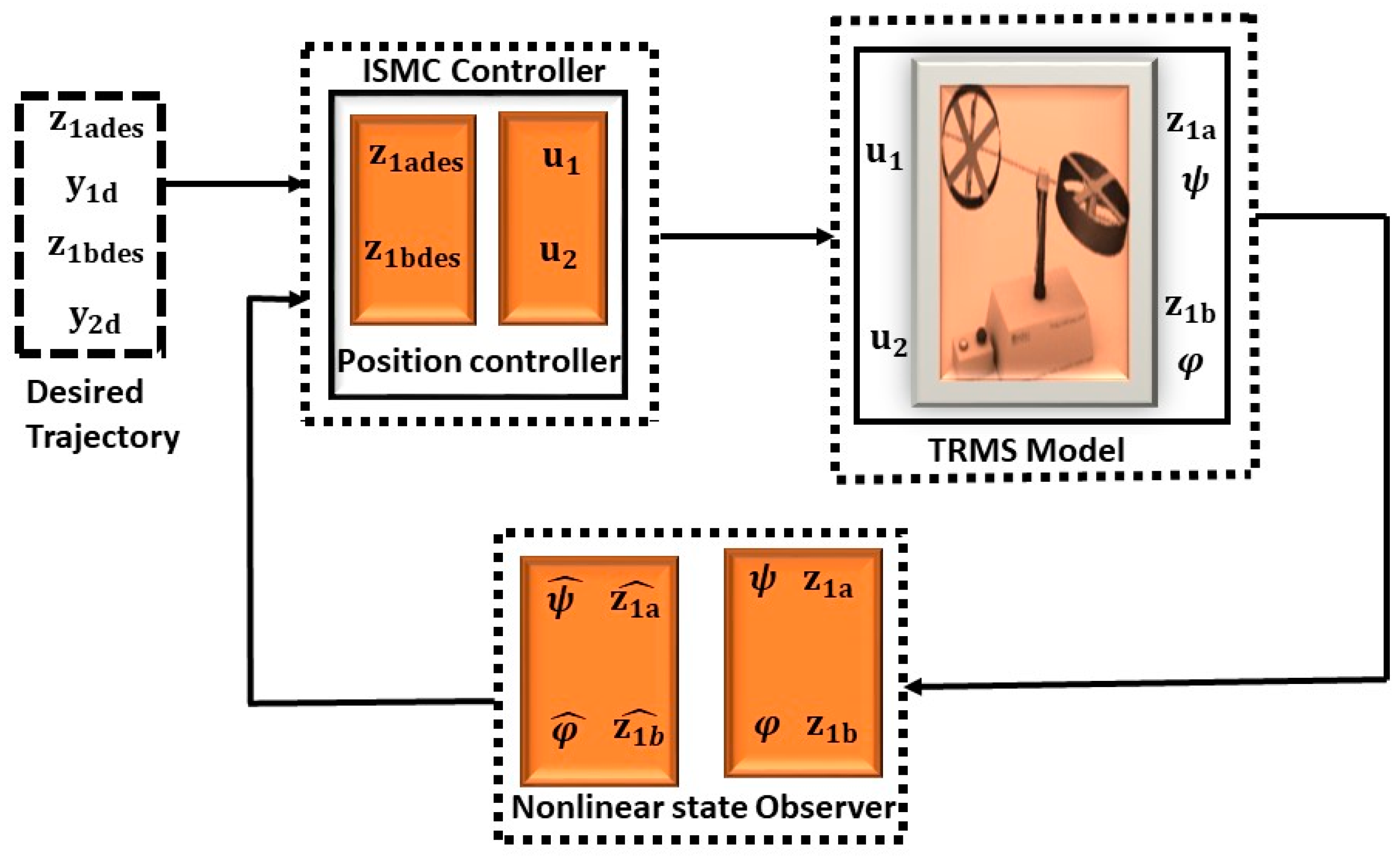
3.2. Integral Sliding Mode Control

The SMC law has the potential advantages of order rejection, insensitivity to parametric variations, and the rejection of external disturbances. However, this control technique suffers from a high-frequency chattering problem that occurs in the control input, which may damage the life of the actuators. Therefore, an SMC-based control technique is proposed to handle this problem, and the ISMC effectively avoids the singularity problem arising in the TSMC law [26]. Furthermore, robustness and fast convergence performance are achieved through the ISMC. Considering the defined dynamic errors for the pitch and azimuth angles, accurate desired trajectories can be obtained by selecting accurate surfaces. The sliding surface for the pitch angle is defined as

$$S_x=c_1{e}_1+c_2{e}_2+Z_{3a}+c\int e_1(t)$$

(27)

where $c$, $c_1$ and $c_2$ are the positive constant, i.e., ${c,c}_1,c_2>0$, and integral action in the sliding surface is used to minimize the steady error. After differentiation $S_x$ can be expressed as

$$\dot{S_{\mathrm{x}}}=c_1\left({\dot{\mathsf{\phi }}}_1-{{\dot{\mathsf{\phi }}}_1}_d\right)+c_2\left({\dot{\mathsf{\phi }}}_2-{{\dot{\mathsf{\phi }}}_2}_d\right)+{\dot{Z}}_{3a}+c{e}_1\left(t\right)$$

(28)

The equivalent control part is computed by substituting ${\dot{Z}}_{3a}$ from Equation (12) into (28). The $u_{1eq}$ changes as follows:

$$u_{1eq}={\displaystyle \frac{-T_{11}}{K_1}}\left(c_1\left({\omega }_x-{{\dot{\mathsf{\phi }}}_1}_d\right)+c_2\left({\dot{\mathsf{\phi }}}_2-{{\dot{\mathsf{\phi }}}_2}_d\right)-{\displaystyle \frac{T_{10}}{T_{11}}}{Z}_{3a}+c{e}_1(t)\right)$$

(29)

where the reachability control law is given by $u_{1dis}=-{\mathrm{ɳ}}_{1}sign\left(S_{\mathrm{x}}\right)-{\zeta }_1{S}_{\mathrm{x}}$. Consequently, the overall controller for ISMC law on the horizontal plan movement is designed as follows:

$$u_{1app=}{\displaystyle \frac{-T_{11}}{K_1}}\left(c_1\left({\omega }_x-{{\dot{\mathsf{\phi }}}_1}_d\right)+c_2\left({\dot{\mathsf{\phi }}}_2-{{\dot{\mathsf{\phi }}}_2}_d\right)-{\displaystyle \frac{T_{10}}{T_{11}}}{Z}_{3a}+c{e}_1(t)\right)-{\mathrm{ɳ}}_{1}sign\left(S_x\right)-{\zeta }_1{S}_{\mathrm{x}}$$

(30)

Similarly, the sliding surface for vertical plan can be written as

$$S_y=c_3{e}_3+c_4{e}_4+Z_{3b}+\widehat{c}\int e_2(t)$$

(31)

where $\widehat{c},$ $c_3{c}_4>0$, which, after differentiating Equation (31), becomes

$$\dot{S_y}=c_3({\psi }_4-{\dot{\psi }}_{3d})+c_4({\dot{\psi }}_4-{\dot{\psi }}_{4d})+{\dot{Z}}_{3b}+\widehat{c}{e}_2\left(t\right)$$

(32)

Considering the sliding surface $\dot{S_y}=0$, the equivalent control $u_{2eq}$ can be computed by substituting the value of ${\dot{Z}}_{3b}$ from Equation (13) in (32) as follows:

$$u_{2eq}={\displaystyle \frac{-T_{21}}{K_2}}\left(c_3\left({\omega }_y-{\dot{\psi }}_{3d}\right)+c_4\left({\dot{\psi }}_4-{\dot{\psi }}_{4d}\right)-{\displaystyle \frac{T_{20}}{T_{21}}}{Z}_{3b}+\widehat{c}{e}_1(t)\right)$$

(33)

whereas the discontinuous law is $u_{2dis}=-{\mathrm{ɳ}}_{2}sign\left(S_{\mathrm{y}}\right)-{\zeta }_2{S}_{\mathrm{y}}$. The overall control law for the vertical plan movement can be written as

$$u_{2app=}{\displaystyle \frac{-T_{21}}{K_2}}\left(c_3\left({\omega }_y-{\dot{\psi }}_{3d}\right)+c_4\left({\dot{\psi }}_4-{\dot{\psi }}_{4d}\right)-{\displaystyle \frac{T_{20}}{T_{21}}}{Z}_{3b}+\widehat{c}{e}_1(t)\right)-{\mathrm{ɳ}}_{2}sign\left(S_{\mathrm{y}}\right)-{\zeta }_2{S}_{\mathrm{y}}$$

(34)

where ${\mathrm{ɳ}}_1$, ${\mathrm{ɳ}}_2$ ${\zeta }_1$, ${\zeta }_2$, $c_1$, $c_1$, $c_3$, $c_4$, $c$ and $\widehat{c}$ are the controller tuning parameters and are selected in such a way that the Lyapunov functions $L_X$ and $L_y$ remain negative definite. Table 3 presents details of the tuning parameters.

Theorem 2.

By considering the system dynamics outlined in Equations (12) and (13) and the assumptions mentioned earlier, the robust control laws (29) and (33) along with the strong reachability laws have been designed. Additionally, the proposed control laws ensure finite-time convergence for the ISMC.

Proof. 

To prove the Lyapunov stability test, this section explains the Lyapunov stability criterion for the existence and convergence of ISMC. The LCF for pitch angle is given by

$$L_X={\displaystyle \frac{1}{2}}{S}_x^2$$

(35)

After differentiating Equation (35), we obtain

$${\dot{L}}_x=S_x{\dot{S}}_x$$

(36)

Substituting Equation (28) into (35), and after simplifying, the above equation can be expressed as

$$\begin{gathered} {\dot{L}}_x=S_x(-{\mathrm{ɳ}}_{1}sign\left(S_x\right)-{\zeta }_1{S}_x) \\ {\dot{L}}_x\le -{\mathrm{ɳ}}_1\left|S_x\right|-{\zeta }_1{S}_x^2 \end{gathered}$$

(37)

The LCF for the yaw angle is considered as

$$L_y={\displaystyle \frac{1}{2}}{S}_y^2$$

(38)

Taking the time derivative and substituting the value of value of $\dot{S_y}$ from Equation (32), we obtain

$$\begin{gathered} {\dot{L}}_y=S_y(-{\mathrm{ɳ}}_{2}sign\left(S_y\right)-{\zeta }_2{S}_y) \\ {\dot{L}}_y\le -{\mathrm{ɳ}}_2\left|S_{\mathrm{y}}\right|-{\zeta }_2{S}_y^2 \end{gathered}$$

(39)

${\mathrm{ɳ}}_1,{\mathrm{ɳ}}_2$, ${\zeta }_1$ and ${\zeta }_2$ are the positive constant tuning parameters and should be greater than zero, as given in Table 3. All system dynamics for the ISMC converge to the origin within a finite time. □

Remark 2.

The strong reachability law will eliminate high-frequency oscillation, and the chattering problem arises in the control input of pitch and yaw angle, respectively, as presented below:

$$\left\{\begin{array}{c}{u}_{1dis}=-{\zeta }_1{S}_x-{\mathrm{ɳ}}_{1}sign\left(S_x\right)\\ u_{2dis}=-{\zeta }_2{S}_y-{\mathrm{ɳ}}_{2}sign\left(S_y\right)\end{array}\right.$$

where ${\zeta }_1$, ${\zeta }_2$, ${\mathrm{ɳ}}_1$ and ${\mathrm{ɳ}}_2$ are the positive constant.

3.3. Terminal Sliding Mode Control

Compared to the conventional SMC technique, the TSMC law with a terminal surface provides fast and finite-time convergence with high control precision. The chattering problem that occurred in the first-order SMC is also successfully reduced by the TSMC. The fast convergence guarantees that the system states lead to the equilibrium position in finite time by choosing the accurate parameters of the sliding surface, which also enhances the control performance [27]. Compared to SMC, TSMC improves the transient performance and noise problems. To design a robust TSMC control system for TRMS, both system outputs are considered separately, and each sliding surface is proposed for both outputs. In order to achieve convergence and trajectory tracking, the sliding surface for the pitch angle are defined as

$$S_1=c_1{e}_1+c_2{e}_2+Z_{3a}+{\beta }_1{\left|e_1\right|}^{{\displaystyle \frac{p_1}{q_1}}}sign\left(e_1\right)$$

(40)

where $p_1$ and $q_1$ must be odd numbers and $p_1$ should be greater than $q_1$ and ${\beta }_1>0$, while the range of $p_1$ and $q_1$ lies in between zero and one, i.e., $0>{\displaystyle \frac{p_1}{q_1}}<1$. Taking the time derivative of sliding manifold and substituting the value of ${\dot{Z}}_{3a}$ in the above equation, we obtain

$$\begin{gathered} {\dot{S}}_1=c_1\dot{e_1}+c_2\dot{e_1}+{\dot{Z}}_{3a}+{\beta }_1{\gamma }_1{\left|e_1\right|}^{{\gamma }_1-1}{\dot{e}}_1 \\ \dot{S_1}=c_1\left({\mathsf{\phi }}_2-{{\dot{\mathsf{\phi }}}_1}_d\right)+c_2\left({\dot{\mathsf{\phi }}}_2-\dot{{\mathsf{\phi }}_{2d}}\right)-{\displaystyle \frac{T_{10}}{T_{11}}}{Z}_{3a}+{\displaystyle \frac{K_1}{T_{11}}}{u}_1+{\beta }_1{\displaystyle \frac{p_1}{q_1}}{e}^{{\displaystyle \frac{p_1}{q_1}}-1}\dot{e_1} \end{gathered}$$

(41)

After simplification, the equivalent controller is computed as follows:

$$u_{1eq}={\displaystyle \frac{-T_{11}}{K_1}}\left(c_1\left({\omega }_x-{{\dot{\phi }}_1}_d\right)+c_2\left({\dot{\mathsf{\phi }}}_2-{{\dot{\phi }}_2}_d\right)-{\displaystyle \frac{T_{10}}{T_{11}}}{Z}_{3a}+{\beta }_1{\displaystyle \frac{p_1}{q_1}}{e}^{{\displaystyle \frac{p_1}{q_1}}-1}\dot{e_1}\right)$$

(42)

The strong reachability law is expressed as $u_{1dis}=-{\zeta }_1{S}_1-k_{1}sign\left(S_1\right)$. The combined equivalent and discontinuous controller part for the pitch angle are presented by

$$u_{1app}={\displaystyle \frac{-T_{11}}{K_1}}\left(c_1\left({\omega }_x-{{\dot{\mathsf{\phi }}}_1}_d\right)+c_2\left({\dot{\mathsf{\phi }}}_2-{{\dot{\mathsf{\phi }}}_2}_d\right)-{\displaystyle \frac{T_{10}}{T_{11}}}{Z}_{3a}+{\beta }_1{\displaystyle \frac{p_1}{q_1}}{e}^{{\displaystyle \frac{p_1}{q_1}}-1}\dot{e_1}\right)-{\zeta }_1{S}_1-k_{1}sign\left(S_1\right)$$

(43)

The sliding surface for the yaw angle is given by

$$S_2=c_3{e}_3+c_4{e}_4+Z_{3b}+{\beta }_2{\left|e_1\right|}^{{\displaystyle \frac{p_2}{q_2}}}sign\left(e_2\right)$$

(44)

The derivative of Equation (44) becomes

$${\dot{S}}_2=c_3\dot{e_1}+c_2\dot{e_4}+{\dot{Z}}_{3b}+{\beta }_2{\displaystyle \frac{p_2}{q_2}}{e}^{{\displaystyle \frac{p_2}{q_2}}-1}\dot{e_2}$$

(45)

where $p_2$ and $q_2$ must be odd numbers, i.e.,$p_2$ $>q_2$, ${\beta }_2>0$, and the range of $p_1$ and $q_1$ should lie between 0 and 1, i.e., $0>{\displaystyle \frac{p_2}{q_2}}<$ 1. The Equation (45) can be rewritten as

$${\dot{S}}_2=c_3({\psi }_4-{\dot{\psi }}_{3d})+c_4({\dot{\psi }}_4-{\dot{\psi }}_{4d})-{\displaystyle \frac{T_{20}}{T_{21}}}{Z}_{3b}+{\displaystyle \frac{K_2}{T_{21}}}{u}_2+{\beta }_2{\displaystyle \frac{p_2}{q_2}}{e}^{{\displaystyle \frac{p_2}{q_2}}-1}\dot{e_2}$$

(46)

The equivalent control part for pitch angle can be computed as follows:

$$u_{2eq}={\displaystyle \frac{-T_{21}}{K_2}}\left(c_3\left({\omega }_y-{\dot{\psi }}_{3d}\right)+c_4\left({\dot{\psi }}_4-{\dot{\psi }}_{4d}\right)-{\displaystyle \frac{T_{20}}{T_{21}}}{Z}_{3b}+{\beta }_2{\displaystyle \frac{p_2}{q_2}}{e}^{{\displaystyle \frac{p_2}{q_2}}-1}\dot{e_2}\right)$$

(47)

where the discontinuous controller can be written as $u_{2dis}=-{\zeta }_2{S}_2-k_{2}sign\left(S_2\right)$. The overall controller for yaw angle can be expressed as

$$u_{2app}={\displaystyle \frac{-T_{21}}{K_2}}\left(c_3\left({\omega }_y-{{\dot{\mathsf{\phi }}}_1}_d\right)+c_4\left({\dot{\psi }}_4-{{\dot{\mathsf{\phi }}}_2}_d\right)-{\displaystyle \frac{T_{20}}{T_{21}}}{Z}_{3b}+{\beta }_2{\displaystyle \frac{p_2}{q_2}}{e}^{{\displaystyle \frac{p_2}{q_2}}-1}\dot{e_2}\right)-{\zeta }_2{S}_2-k_{2}sign\left(S_2\right)$$

(48)

where the controller tuning parameters are ${\zeta }_1$, ${\zeta }_2$, $k_1$,$k_2$, $c_1$, $c_2$, $c_3$, $c_4$ and $\widehat{c}$. These parameters are selected in such a way that the Lyapunov functions $L_n$ and $L_m$ remain negative definite. The Lyapunov stability analysis for the TSMC is as follows:

Theorem 3.

Considering the system dynamics described by Equations (12) and (13) and the previously stated assumptions, robust control laws (42) and (47) have been formulated alongside strong reachability laws. Furthermore, the subsequent proposed control laws guarantee finite-time convergence of the TSMC law.

Proof. 

For the Lyapunov stability test, consider the augmented LCF for the pitch angle as

$$L_n={\displaystyle \frac{1}{2}}{S}_1^2$$

(49)

Taking the time derivative of Equation (49), and substituting (41) into (49), we obtain

$${\dot{L}}_n=S_1(-k_{1}sign\left(S_1\right)-{\zeta }_1{S}_1)$$

(50)

where

$${\dot{L}}_n\le -k_1\left|S_1\right|-{\zeta }_1{S}_1^2$$

(51)

The LCF for the yaw angle is chosen as

$$L_{\mathrm{m}}={\displaystyle \frac{1}{2}}{S}_2^2$$

(52)

Differentiating Equation (52), we obtain

$$\begin{gathered} {\dot{L}}_m=S_2{\dot{S}}_2 \\ {\dot{L}}_m=S_2(-k_{2}sign\left(S_2\right)-{\zeta }_2{S}_2) \end{gathered}$$

(53)

Equation (53) can be rewritten as

$${\dot{L}}_m\le -k_2\left|S_2\right|-{\zeta }_2{S}_2^2$$

(54)

where $k_1,{\zeta }_1,k_2$ and ${\zeta }_2$ are positive constants and must be greater than zero. Thus, the derivatives of ${\dot{L}}_{\mathrm{n}}$ and ${\dot{L}}_{\mathrm{m}}$ become negative definite and the dynamics of TSMC converge to an origin over a finite time. □

3.4. Uniform Robust Exact Differentiator

This section introduces the URED for estimating the higher derivative terms in the aerodynamics of TRMS. URED is used to derive the position states of the system. To formulate a URED observer, it is assumed that a signal $f\left(t\right)$, defined over the interval $[0,\mathrm{\infty }]$, is a measureable function. Additionally, it is decomposed into sub parts $f\left(t\right)=f_0\left(t\right)+v\left(t\right)$, where $f_0\left(t\right)$ represents the base function that can be further differentiated twice, and $v\left(t\right)$ illustrates the uniformly bounded signal. Considering that ${\overline{e}}_1=f_0\left(t\right)$ and ${\dot{\overline{e}}}_1={\dot{f}}_0\left(t\right)$, the state space representation for base signal can be articulated as

$${\dot{\overline{e}}}_1={\overline{e}}_2, {\dot{\overline{e}}}_1={\ddot{f}}_0$$

To achieve precise estimation of the first derivative of the base signal, a base sensor is employed. An injection term is utilized to incorporate the information from the actual measurement of the base signal $f_0\left(t\right)$, without a dependence on the initial condition of system dynamics. The following algorithms are presented to ensure accurate estimation:

$$\begin{gathered} {\dot{Z}}_0=-k_1{\phi }_1\left({\overline{\sigma }}_0\right)+Z_1 \\ {\dot{Z}}_1=-k_2{\phi }_2\left({\overline{\sigma }}_0\right) \end{gathered}$$

(55)

where ${\overline{\sigma }}_0=Z_0-f\left(t\right)$ and $k_1,k_2$ represent the optimized tuning parameters. We employed an iterative process to refine the tuning parameters $k_1, k_2$, and $\mu$ in the URED algorithm. Each iteration focused on key performance indicators, such as system stability, response time, and accuracy of derivative estimation. The compensator is adjusted to meet control objectives, particularly in terms of higher-order derivative estimation and ensuring stable pitch and yaw angle behavior.

The value ${\phi }_1$ and ${\phi }_2$ can be expressed as follows:

$$\begin{gathered} {\phi }_1\left({\overline{\sigma }}_0\right)={‖{\overline{\sigma }}_0‖}^{{\displaystyle \frac{1}{2}}}sign\left({\overline{\sigma }}_0\right)+\mathsf{\mu }{\left|{\overline{\sigma }}_0\right|}^{{\displaystyle \frac{3}{2}}}sign({\overline{\sigma }}_0) \\ {\phi }_2\left({\overline{\sigma }}_0\right)={\displaystyle \frac{1}{2}}sign\left({\overline{\sigma }}_0\right)+2\mathsf{\mu }{\overline{\sigma }}_0+{\displaystyle \frac{3}{2}}{\mathsf{\mu }}^2{\left|{\overline{\sigma }}_0\right|}^{2}sign\left({\overline{\sigma }}_0\right) \end{gathered}$$

(56)

When the original arbitrary differentiator is simplified by considering $\mathsf{\mu }=0$ and higher degree terms ${\left|{\overline{\sigma }}_0\right|}^{{\displaystyle \frac{3}{2}}}sign({\overline{\sigma }}_0)$ and ${\left|{\overline{\sigma }}_0\right|}^{2}sign\left({\overline{\sigma }}_0\right)$, it ensures uniform convergence of the states. The convergence time is bounded by the independent initial conditions of the differentiator. Integration terms $Z_0$ and $Z_1$ are utilized for the estimation of $f_0\left(t\right)$ and ${\dot{f}}_0\left(t\right)$. The pitch angle estimated states are as follows: $e_{pitch}=Z_{2a}-{\widehat{Z}}_{2a}$; the yaw angle estimation is expressed as $e_{yaw}=Z_{2b}-{\widehat{Z}}_{2b}$. Here, ${\ddot{Z}}_{2a}$ and ${\ddot{Z}}_{2b}$ represent the second-order derivative of outputs $Z_{2a}$ and $Z_{2b}$, respectively.

Assumption 4.

It is assumed that the actual positions of TRMS, denoted by $(Z_{1a}, Z_{1b})$, as well as their desired position $(Z_{1ades}, y_{1d}, Z_{2ades}, y_{2d})$, along with their first and second differentiators, are measurable.

Nonlinear State Feedback Observer Design Using the Luenberger Technique

The application of the Luenberger method facilitates the design of a nonlinear state feedback observer for a TRMS, with the aim of altering system coordinates and mitigating noise in position sensors. Specifically, under Lipschitz conditions and certain assumptions, a state observer for a nonlinear system is formulated. This involves considering the state space representation of the nonlinear system as follows:

$$\begin{gathered} \dot{x}=f\left(z\right)+g\left(z\right)u+d \\ y=h\left(z\right) \end{gathered}$$

(57)

Given $z \mathsf{ϵ}{R}^n$ and $y$ represent the system outputs, assume that $h\left(0\right)=0$ and $f\left(0\right)=0$ denote the equilibrium position for the unforced system and $d \mathsf{ϵ}{R}^6$ represents the disturbances in TRMS. The nonlinear system described in Equation (57) exhibits a relative degree of $m$ at $z=0$, provided that smooth function ${\overline{\sigma }}_i\left(z\right)=0$ exists, where $i=1,\dots \dots ,\mathrm{m}$, such that

$$\begin{gathered} h\left(z_{1a}\right)=\psi \left(z\right)+{\sigma }_0(z_{1a},u_a) \\ h\left(z_{1a}\right)=\psi \left(z\right)+{\sigma }_0(z_{1a},u_a) \\ L\psi \left(z\right)=b\left(z_{1a}\right)+a\left(z_{1a}\right)u_{a+}{\sigma }_0\left(z_{1a},u_a\right) \\ L\phi \left(z\right)=b\left(z_{1b}\right)+a\left(z_{1b}\right)u_{b+}{\sigma }_0(z_{1b},u_b) \end{gathered}$$

(58)

whereas

$$f(z)=\left[\begin{array}{c}{\displaystyle \frac{a_1}{I_1}}{Z}_{3a}^2+{\displaystyle \frac{b_1}{I_1}}{Z}_{3a}-{\displaystyle \frac{M_g}{I_1}}\sin \left(Z_{1a}\right)-{\displaystyle \frac{B_1\psi }{I_1}}{Z}_{2a}\\ {\displaystyle \frac{a_2}{I_2}}{Z}_{3b}^2+{\displaystyle \frac{b_2}{I_2}}{Z}_{3b}-{\displaystyle \frac{B_{1\phi }}{I_2}}{Z}_{2b}-{\displaystyle \frac{K_c}{I_2}}{1.75(a}_1{Z}_{2b}^2+b_1{Z}_{2b})\end{array}\right]$$

(59)

$$g(z)=\left[\begin{array}{ccc}0& 0& \begin{array}{ccc}0& 0& \begin{array}{cc}{\displaystyle \frac{K_1}{T_{11}}}& 0\end{array}\end{array}\\ 0& 0& \begin{array}{ccc}0& 0& \begin{array}{cc}0& {\displaystyle \frac{K_2}{T_{21}}}\end{array}\end{array}\end{array}\right], h\left(z\right)=\left[\begin{array}{ccc}\begin{array}{c}1\\ 0\end{array}& \begin{array}{c}0\\ 0\end{array}& \begin{array}{ccc}\begin{array}{c}0\\ 1\end{array}& \begin{array}{c}0\\ 0\end{array}& \begin{array}{c}0\\ 0\end{array}\end{array}\end{array}\right]$$

The state observer equation is defined as follows:

$$\widehat{\dot{z}}\left(t\right)=f(\widehat{z}\left(t\right)+g(\widehat{z}\left(t\right)u\left(t\right)+{\left[{\displaystyle \frac{\partial \psi ,\phi (\widehat{z}\left(t\right)}{\partial \widehat{x}}}\right]}^{-1}L(y-h(\widehat{z}\left(t\right))$$

(60)

where $L$ represents the observer parameters matrix, while $\psi \left(z_{1a}\right)$, $\phi \left(z_{1b}\right)$, ${\sigma }_0(z_{1a},u_a)$ and ${\sigma }_0(z_{1b},u_b)$ denote the parameters of the horizontal and vertical subsystem, respectively. The resulting final observer equations for the decoupled TRMS vertical and horizontal subsystems are as follows:

$$\begin{gathered} {\widehat{\dot{z}}}_{1a}=f_a\left({\widehat{z}}_{1a}\right)+g_a\left({\widehat{z}}_{1a}\right)+{\left[{\displaystyle \frac{\partial \psi {\widehat{(z}}_{1a})}{\partial {\widehat{z}}_{1a}}}\right]}^{-1}L(z_{1a}-{\widehat{z}}_{1a}) \\ {\widehat{\dot{z}}}_{1b}=f_b\left({\widehat{z}}_{1b}\right)+g_b\left({\widehat{z}}_{1b}\right)+{\left[{\displaystyle \frac{\partial \psi {\widehat{(z}}_{1b})}{\partial {\widehat{z}}_{2b}}}\right]}^{-1}L(z_{1b}-{\widehat{z}}_{1b}) \end{gathered}$$

(61)

Furthermore, the nonlinear state feedback observer designed using the Luenberger technique is fine-tuned through a combination of theoretical considerations and empirical adjustment. Parameters such as $L$, the observer gain, are optimized to ensure accurate decoupling of the vertical and horizontal subsystems while minimizing the impact of sensor noise. Figure 4 presents the close loop state feedback observer for ISMC as presented below:

4. Simulation Results

This section presents the simulations of the three different robust control techniques, URED, and the state feedback observer for TRMS. Nonlinear control strategies and a state feedback observer were used to evaluate system performance for stable flight testing. All simulations were performed using the MATLAB/Simulink environment with the software R2022b with a DESKTOP-VISCUS 13th Gen Intel(R) Core (TM) i7-13700H, 64-bit operating system, along with the presence of matched disturbances. Simulation run times of $t=15 \mathrm{s}$ and $t=20 \mathrm{s}$ were considered with and without disturbances, respectively, while simulation run times of $t=50 \mathrm{s}$ and $t=20 \mathrm{s}$ were considered for tracking against the reference sinusoidal and step input trajectories. In the next section, a feedback instrument (TRMS 33-220) was used to verify the effectiveness of the proposed controllers. System dynamics Equations (12) and (13) were considered as $Z \mathsf{ϵ}{\mathbb{R}}^6$, $u \mathsf{ϵ}{\mathbb{R}}^2$ and $y \mathsf{ϵ}{\mathbb{R}}^2$, which represent the state inputs and output vectors.

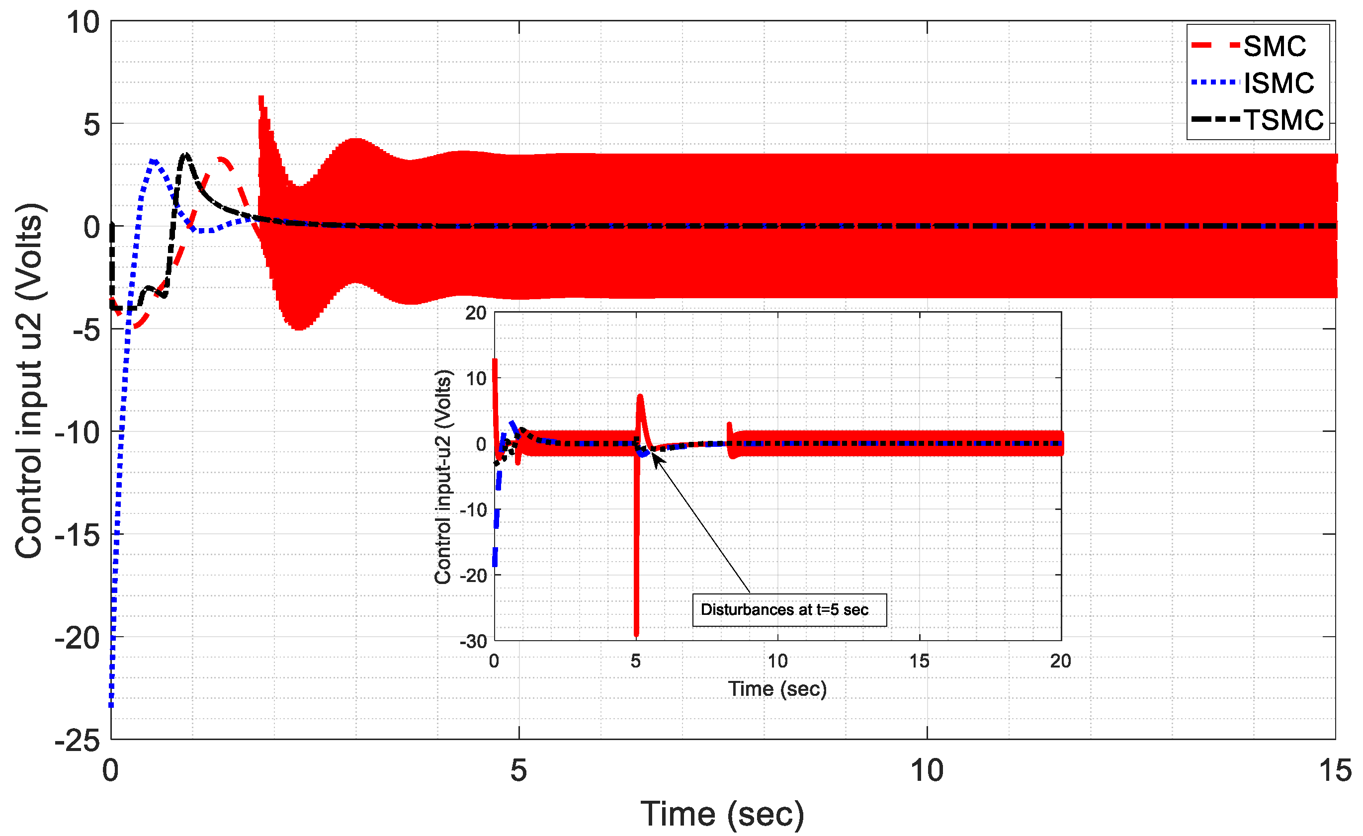
4.1. Case 1: Trajectory Tracking with Disturbances

In this case, the flight behavior of TRMS and effectiveness of the proposed control strategies are compared with each other by incorporating the disturbance for both the horizontal and vertical plan movements in order to check the path following of the desired trajectories. The obtained results are compared based on the transient performance of the SMC, ISMC, and TSMC laws. To evaluate the robust performance and comparison of the controller design in Section 3, disturbances were applied to the aerodynamics of the system at $t=5 \mathrm{s}$ to overcome the model uncertainties and unmeasurable disturbances for a closed-loop system. Figure 5, Figure 6, Figure 7, Figure 8, Figure 9 and Figure 10 show the simulation results of all proposed control techniques. To demonstrate the effectiveness of the proposed method, simulation results were compared to examine the performance of all the proposed control techniques.

Figure 5 and Figure 6 illustrate the trajectory tracking and stability behavior of the pitch and yaw angles along with the addition of disturbances, respectively. As shown in Figure 4, the response of the pitch angle is achieved against the proposed control algorithms. The implemented techniques exhibit smooth performance for a closed-loop system. The SMC stabilized the pitch orientation movement in 4.2 s while ISMC and TSMC took 3.8 s and 3.3 s, correspondingly. The SMC law demonstrated a slight overshoot and undershoot of less than 1%, whereas the other two control techniques showed very good convergence responses with small steady-state error, and the rise time was almost zero. The subplot of Figure 5 demonstrates the pitch angle response for the proposed techniques after the addition of disturbances, with settling times of 5.5 s, 2.9 s, and 3.2 s, respectively, to reach at the desired trajectory. SMC shows minimal steady-state error and overshoot after the disturbance, whereas the ISMC and TSMC laws exhibit smooth transient performance. It can be seen that the proposed controllers reject the effect of disturbances at 12, 7 and 8 s.

Figure 6 presents the convergence response of yaw angle movement together with addition of disturbances, and it can be observed that settling times of 3.5 s, 2.9 s and 3.1 s are observed for SMC, ISMC and TSMC, respectively, to stabilize the yaw angle movement. All the developed algorithms show significantly zero steady-state error, rise time, and overshoot, indicating an almost perfect response and guaranteeing the successful execution of the proposed control schemes on TRMS for the experiment. It could also be observed, initially, that the yaw angle deviated from the desired position owing to parametric perturbation. However, owing to the action of the proposed controllers, both output angles quickly regained the desired trajectories. Subplot of Figure 6 depicts the yaw angle response with disturbances. It can be noticed that the proposed control strategies kept the yaw angle stable after settling times of 7 s, 3.5 s, and 4 s for the SMC, ISMC and TSMC, respectively. The simulation results for both outputs show that all controllers have the capability to reject the external perturbation and maintain the robustness of the system. Moreover, the proposed design techniques with the application of undesired external disturbances and uncertainties took the system into the zero position within a finite time.

Figure 7 and Figure 8 demonstrate the control input effort for the output angles. It can be noticed that the SMC produces very high-frequency oscillation and chattering phenomena in both the control inputs. The oscillation can drastically decrease the health of actuators and degrade the system dynamic performance; therefore, in a counterpart, the ISMC and TSMC laws adequately produce chattering-free control input with a reasonable magnitude, which can be considerable for real-time implementation. Moreover, the ISMC and TSMC laws aim to reduce chattering when compared with the traditional SMC in a more precise continuous and less oscillatory response. The obtained results demonstrate that system errors converge within a finite time towards the equilibrium position while reaching the sliding manifold. The subplots in Figure 7 and Figure 8 show the control input performance for the implemented control strategies. Disturbances are added to both control inputs at $t=5 \mathrm{s}$. It can be seen that the SMC initially produced a large spike, while ISMC and TSMC illustrated very good responses and kept the control efforts at the desired position. Designed integral and terminal sliding surfaces accumulate over time and help the system to recover from external disturbances and uncertainties.

In the presence of disturbances, the mathematical representation for vertical and horizontal planes can be represented as follows:

$$\left\{\begin{array}{c}{\dot{Z}}_{1a}=Z_{2a}\\ {\dot{Z}}_{2a}={\displaystyle \frac{a_1}{I_1}}{Z}_{3a}^2+{\displaystyle \frac{b_1}{I_1}}{Z}_{3a}-{\displaystyle \frac{M_g}{I_1}}\sin \left(Z_{1a}\right)-{\displaystyle \frac{B_1\psi }{I_1}}{Z}_{2a}+d_{2a}(t)\\ {\dot{Z}}_{3a}=-{\displaystyle \frac{T_{10}}{T_{11}}}{Z}_{3a}+{\displaystyle \frac{K_1}{T_{11}}}{u}_1+d_{3a}(t)\end{array}\right.$$

$$\left\{\begin{array}{c}{\dot{Z}}_{1a}=Z_{2a}\\ {\dot{Z}}_{2a}={\displaystyle \frac{a_1}{I_1}}{Z}_{3a}^2+{\displaystyle \frac{b_1}{I_1}}{Z}_{3a}-{\displaystyle \frac{M_g}{I_1}}\sin \left(Z_{1a}\right)-{\displaystyle \frac{B_1\psi }{I_1}}{Z}_{2a}+d_{2a}(t)\\ {\dot{Z}}_{3a}=-{\displaystyle \frac{T_{10}}{T_{11}}}{Z}_{3a}+{\displaystyle \frac{K_1}{T_{11}}}{u}_1+d_{3a}(t)\end{array}\right.$$

where $d_{2a}(t)$, $d_{2b}\left(t\right)$, $d_{3a}\left(t\right)$, and $d_{3b}\left(t\right)$ represent the disturbances affecting the pitch and yaw angles along with the control inputs, $u_1$ and $u_2$, which counteract these disturbances and maintain the stability of TRMS, where $d$ is the disturbance defined as

$$d(t-5)=\left\{\begin{array}{c}0 t\ne 5\\ 1 t=5\end{array}\right\}$$

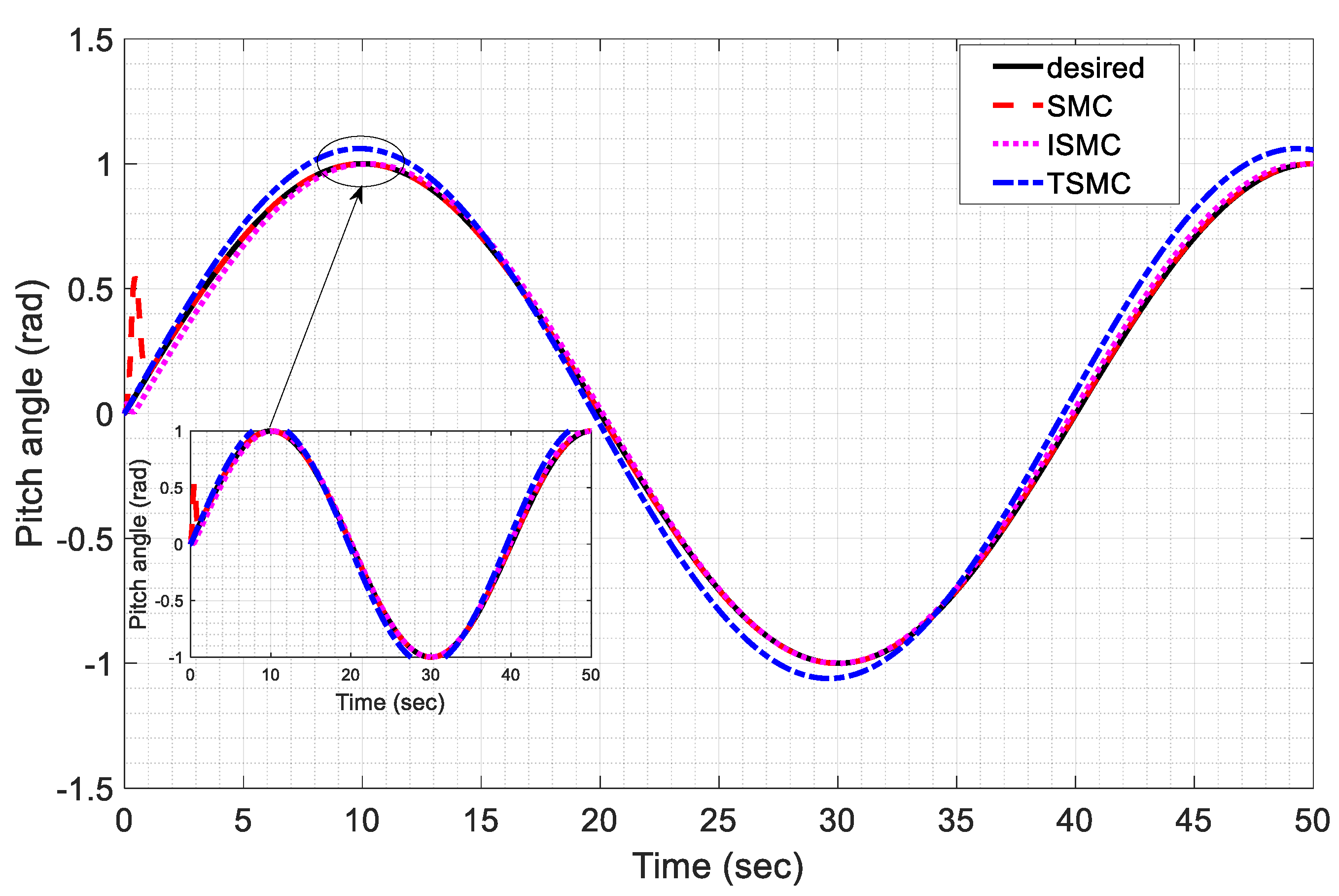
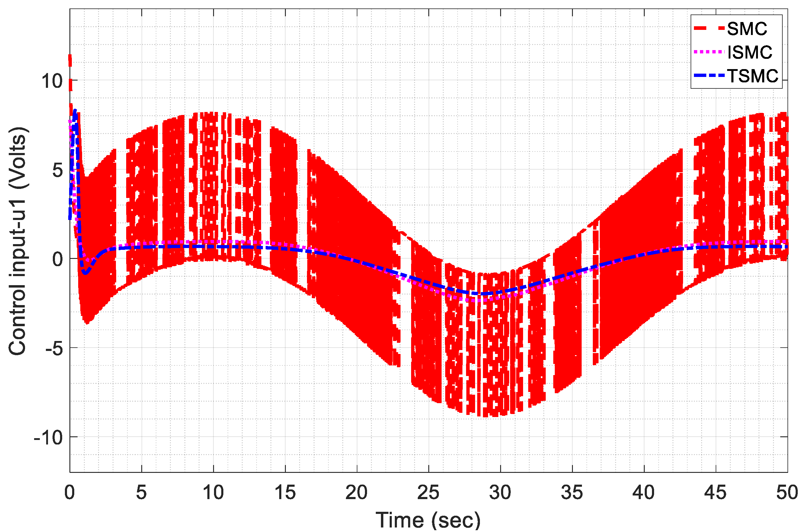
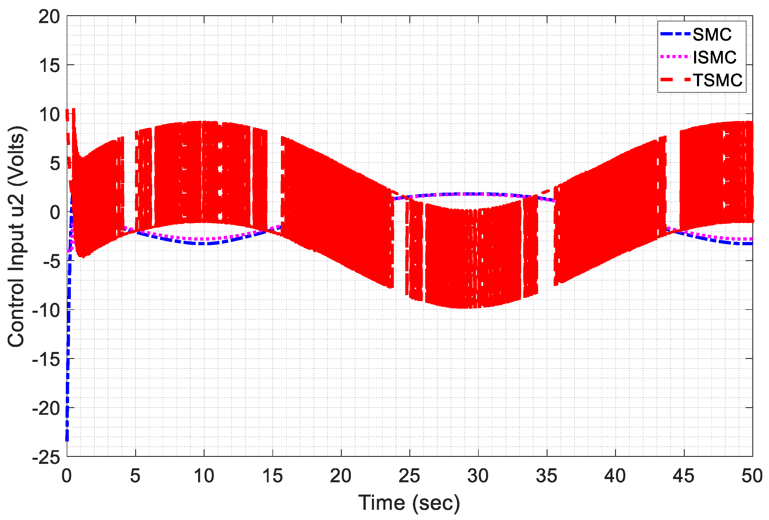
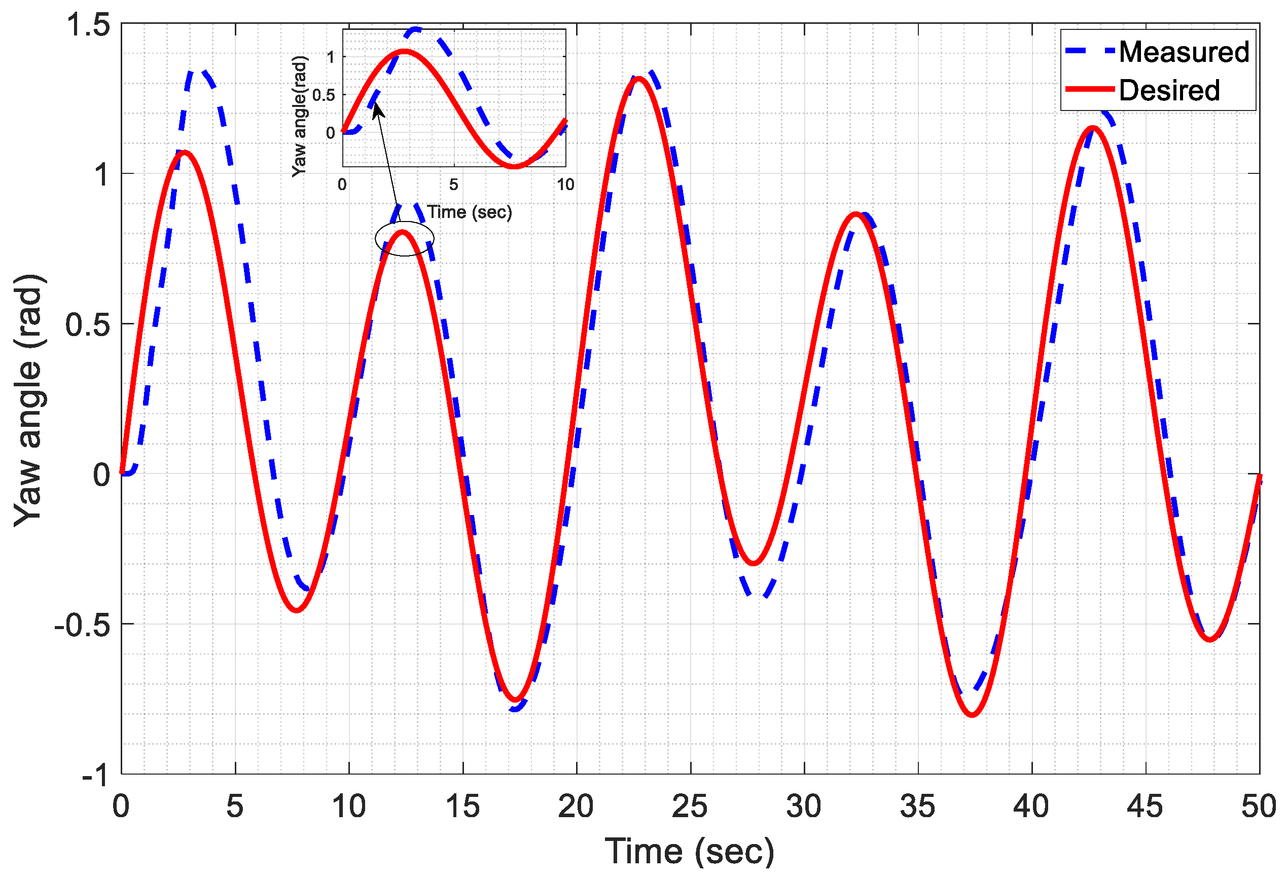
4.2. Case 2: Trajectories Tracking with Sinusoidal Wave

This section presents the simulation results of the SMC, ISMC, and TSMC algorithms for tracking the trajectories of the 2-DOF TRMS against the reference sinusoidal input. The control objective is to minimize the errors between the desired and measured outputs of the system. A sinusoidal input signal is considered for all controllers to evaluate the tracking and stability of the proposed controllers. The desired trajectory is set at time $t=50 \mathrm{s}$ with an amplitude interval of $[-1,1]$ considered for the output of TRMS. Figure 8, Figure 9, Figure 10, Figure 11, Figure 12 and Figure 13 illustrate a comparison of the pitch angle, yaw angle, control inputs, and tracking errors for a TRMS under the newly designed control methods. The desired reference trajectory is chosen as $y_{\mathrm{1,2}d}=\sin (2\pi t)$ radian.

Figure 9 and Figure 10 present the tracking performance of the pitch and yaw angles, respectively, against the reference sinusoidal input signal for the feedback closed-loop controllers. It can be seen that all three controllers show very good tracking performance and stabilize both angles to the reference input within a finite time, and then asymptotically stay in a region of origin. The ISMC performance is much better than that of SMC and TSMC, whereas TSMC exhibits a much more accurate performance than SMC. The SMC law shows more steady-state error and overshoot compared to the other two controllers, and the rise time and setting time of ISMC and TSMC are superior to those of SMC. Compared with the SMC and TSMC techniques, the ISMC law demonstrates fast convergence, almost zero steady-state error, and is close to the reference input for the main and tail rotors.

Table 4. Transient performance analysis for the designed controllers.

	Without Disturbance					With Disturbance
Control Techniques	Euler’s Angles	Settling Time (s)	Rise Time (s)	Overshoot (%)	Steady-State Error (${\mathit{e}}_{\mathit{s}\mathit{s}}$)	Settling Time (s)	Rise Time (s)	Overshoot (%)	Steady-State Error (${\mathit{e}}_{\mathit{s}\mathit{s}}$)
SMC	Pitch	4.5	4	0.15	0.005	7	6	0.1	0.002
	Yaw	3.2	1	0.1	0	6	6.5	0.12	0.009
ISMC	Pitch	2.3	0.6	0.08	0	3.1	1	0.08	0
	Yaw	2.9	0.4	0.01	0	3.3	1.1	0.01	0
TSMC	Pitch	3.1	0.7	0.085	0	3.3	1.3	0.082	0
	Yaw	3.1	0.5	0.02	0	3.4	1.2	0.02	0

presents a detailed analysis of the transient performance of all the controllers against the reference sinusoidal input signal.

Figure 11 and Figure 12 show the control input performance for the horizontal and vertical movements of the motor for the proposed control schemes. It can be noted that SMC produced chattering phenomena in both the control inputs, which are effectively improved by ISMC and TSMC. Mitigating the chattering in ISMC and TSMC for TRMS involves a combination of design techniques and control adjustments. For ISMC, the technique of smooth approximation is employed to reduce chattering by modifying the control law to achieve smoother transitions. In Terminal TSMC, techniques of softened and relaxed terminal sliding modes are utilized to minimize high-frequency oscillations and improve system stability.

Figure 13 and Figure 14 depict the tracking error performance for all control algorithms for pitch and yaw movements, respectively. It can be observed that all errors for each control technique exhibit a smooth finite-time convergence towards the origin. Both surfaces smoothly converged towards the origin, and the obtained results demonstrate that the system errors converge to the zero position while reaching the sliding surfaces.

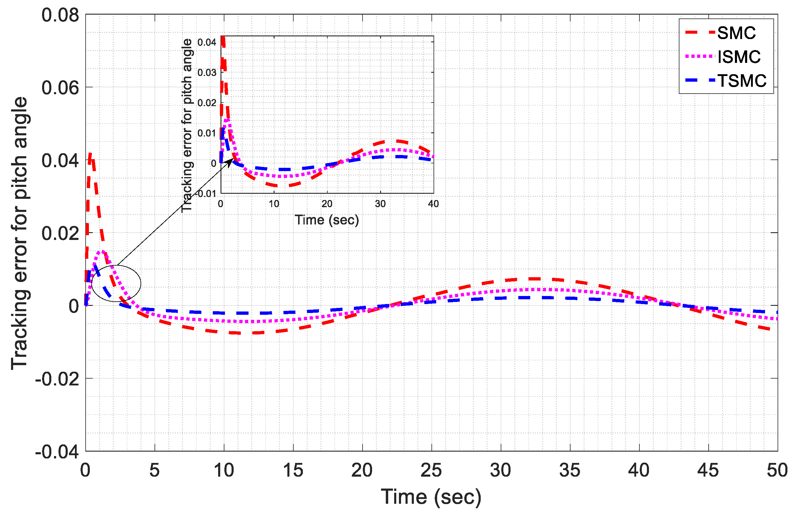
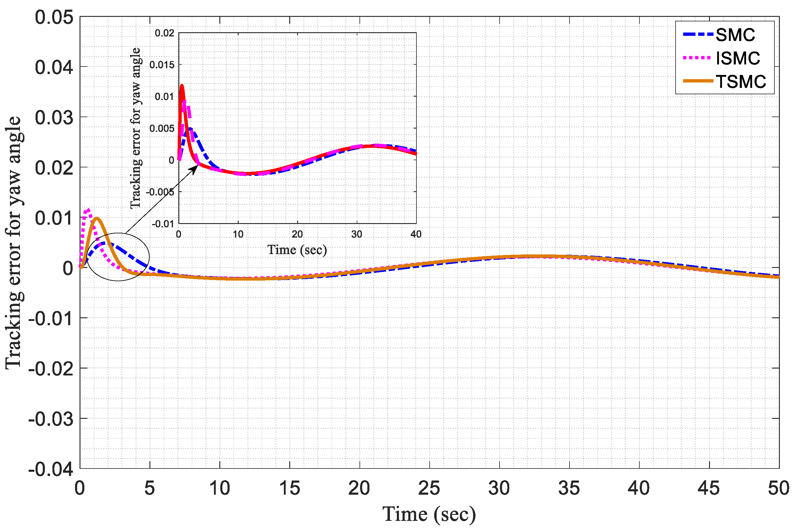
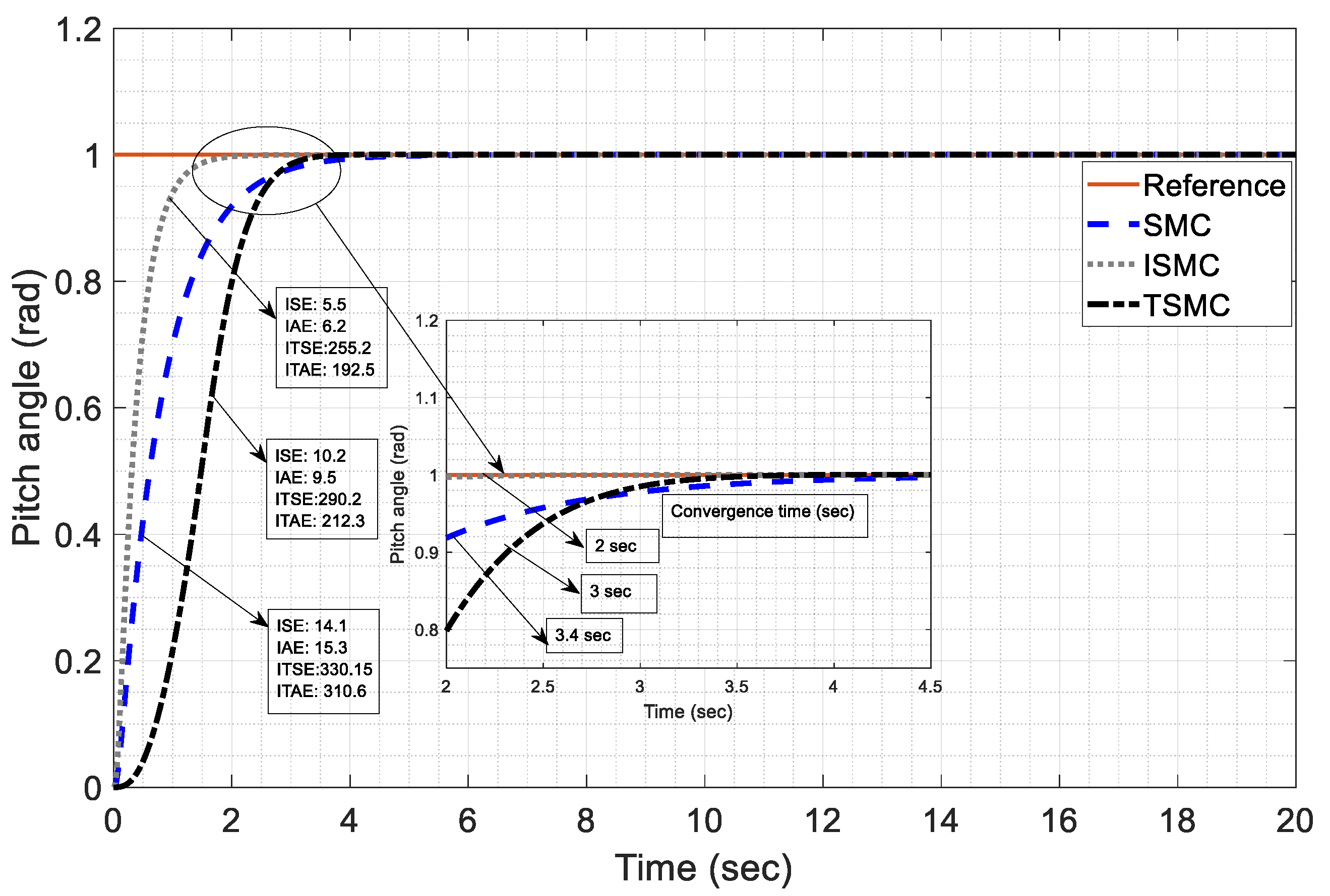
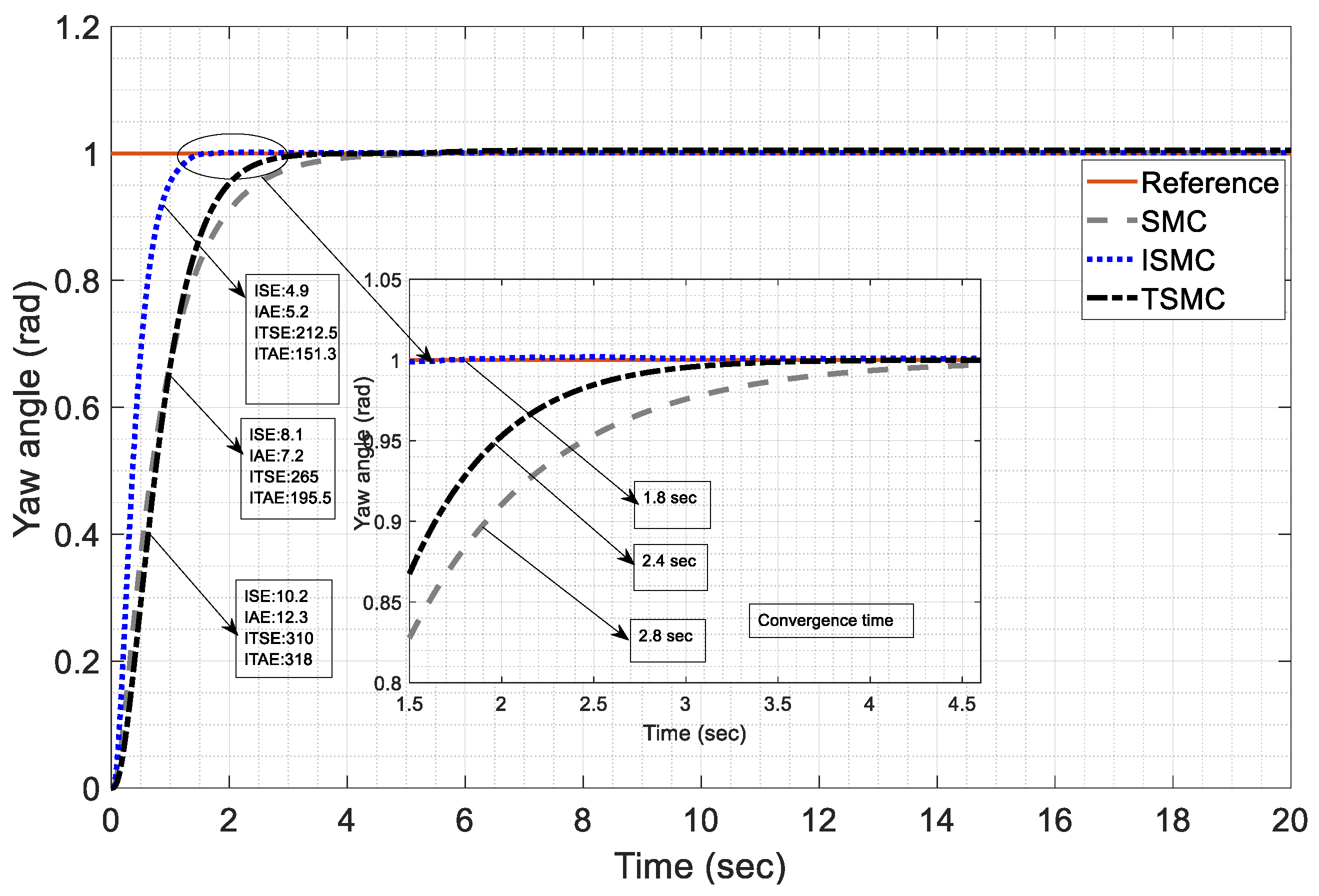
4.3. Case 3: Trajectories Tracking with Reference Step Input

This section presents the simulation-based results of the three design control techniques for tracking TRMS against the reference step input trajectory. It is worth mentioning that our proposed strategies are compared with the Variable Gains SMC (VGSMC), O-SMC, and TSMC-based simulated results in [28,29]. The simulation results presented in Figure 15, Figure 16, Figure 17 and Figure 18 demonstrate that the convergence and tracking performance of TRMS under the newly designed control strategies are significantly improved and faster than those of [28,29].

Figure 15, Figure 16, Figure 17 and Figure 18 represent the tracking response against the step input for the pitch and yaw angles, along with the control inputs. Figure 15 illustrates the pitch angle response for all the proposed controllers. SMC, ISMC, and TSMC have settling times of 2 s, 3 s and 3.4 s, respectively. The SMC requires a longer settling time for the convergence of system trajectories than the TSMC and ISMC laws, whereas the ISMC law shows the best performance with the shortest settling time. It is noteworthy that the reference tracking is very good for all controllers with almost zero steady-state error and overshoot, which demonstrates the effectiveness of the investigated control laws. It can be observed that the proposed SMC and TSMC control laws provide fast convergence and improved settling time with minimum overshoot and steady error compared to the literature counterpart in [28,29]. The performance indices called the Integral Square Error (ISE), Integral Absolute error (IAE), Integral Time Square Error (ITSE), and Integral Time Absolute Error (ITAE) show the best performance for the ISMC law when compared with the SMC and TSMC laws, as shown in the figure below. However, the TSMC law shows better performance than SMC for all the performance indices.

Figure 16 shows the yaw angle response for the SMC, ISMC, and TSMC laws for the step input. The SMC, ISMC, and TSMC required settling time of 1.8 s, 2.4 s and 2.8 s, respectively. It is evident from the obtained response that the performance of the ISMC law is satisfactory. The rise time, steady-state error, and overshoot are zero for all controllers. To demonstrate the effectiveness of the proposed work, the SMC and TSMC laws are compared with those in the literature [28,29]. Both newly designed control laws claimed better finite-time convergence to the equilibrium position than the compared work. The TSMC law shows smooth performance under uncertainties and disturbances compared to the literature presented in [29]. The performance indices indicate that the ISMC exhibits the best performance for IAE, ITSE, ISE, and ITAE, as shown in the figure below.

Figure 17 and Figure 18 illustrate the responses of the control input for the pitch and yaw angles, respectively. The SMC exhibits chattering phenomena in the control input of both angles, which can damage the life of the actuator during the experimental study. Therefore, the ISMC and TSMC are designed to effectively remove the chattering problem. It is clear from the figures below that the control input is nominal for the ISMC and TSMC and is within the bounds of the practical system. The chattering phenomenon that occurred in the proposed work presents less oscillation and peak-to-peak amplitude compared with the literature presented in [28,29]. In addition, our proposed work shows improved chattering performance for both control inputs compared to the VG-SMC, O-SMC, and NTSMC laws presented in [28,29]. In the literature [28], SMC illustrates peak-to-peak voltage amplitude values of 10 volts for pitch angle and 9 volts for yaw angle, whereas the O-SMC in the literature [29] demonstrates peak-to-peak amplitude voltages of 14 volts and 12 volts for both control inputs. However, our proposed work asserts peak-to-peak voltages of 4.8 volts and 3.8 volts for both control inputs, which are better than those reported in the literature.

Table 5. Comparative analysis of proposed control techniques with literature [28,29].

	For Step Input Signal
Control Techniques	Euler’s Angles	Settling Time (s)	Control Input (Volt)	Overshoot (%)	Steady-State Error (${\mathit{e}}_{\mathit{s}\mathit{s}}$)
VGSMC proposed in [25]	Pitch	5	10	0	0.01
	Yaw	3	9	0.1	0
O-SMC proposed in [26]	Pitch	5.2	14	0.05	0.001
	Yaw	4	12	0.02	0.003
NTSMC proposed in [26]	Pitch	4	-	0.01	0
	Yaw	3.5	-	0.02	0
The proposed SMC	Pitch	3.4	4.8	0	0
	Yaw	2.8	3.8	0	0
The proposed TSMC	Pitch	3	-	0	0
	Yaw	2.4	-	0	0

briefly explains the proposed and comparison studies.

Figure 19 displays the outcomes of employing URED to accurately determine the system position states. The URED is adept at precisely measuring the unknown state, specifically the angular velocity information of the system. Figure 20 and Figure 21 illustrate the results of employing a state feedback observer within the context of the ISMC. Figure 20 shows that the design observer effectively monitored and tracked the estimated pitch and yaw angles. The obtained results demonstrate active steering of the trajectories towards the desired positions, ensuring alignment with the intended targets. Figure 21 illustrates the performance of the disturbance observer in response to a step input signal for TRMS. At $t=30 \mathrm{s}$, a disturbance is introduced. Following the disturbance, both the pitch and yaw angles accurately follow the desired trajectories with minimal alterations to the rise time, overshoot, and settling time.

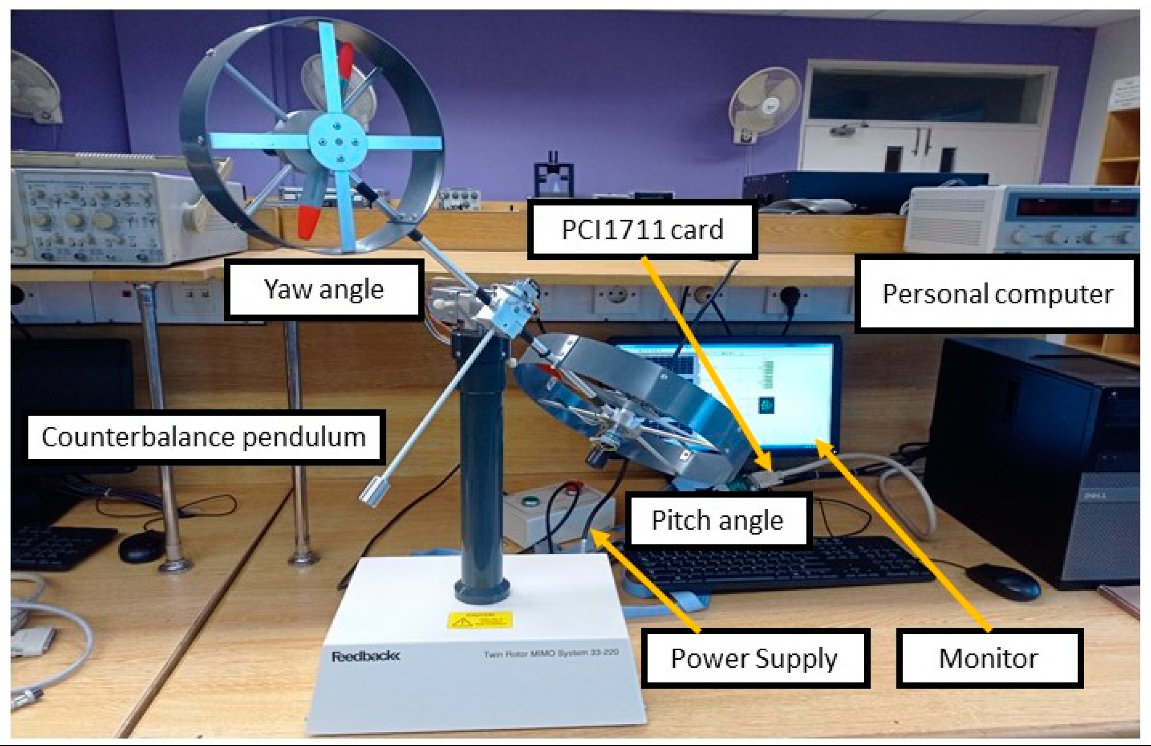
4.4. Experimental Results

The designed control techniques were tested to validate their performances on a TRMS test bench. Figure 22 and Figure 23 present the configuration and environment for the real-time TRMS. A feedback instrument (TRMS 33-220) was used for experimental work and testing of the proposed control schemes. The components used for the experiment were a desktop computer, Advantech PCI1711 card, adaptor cable, feedback cables, and on/off switch box. Initially, real-time implementation of ISMC and TSMC with 2-DOF TRMS using MATLAB/Simulink (2023) with the interfacing of the PCI1711 card was completed. The proposed control scheme was tested using MATLAB/Simulink software along with a PCI1711card, and the PCI card read the encoder channel information in the feedback instrument using digital I/O lines. The PCI card read data from the encoder and converted them into analog-to-digital and digital-to-analog forms. The encoder had two outputs representing the rotor positions on the horizontal and vertical axes. A control signal for both the angles was applied to the block. The attached sensor sensed the positions of the angles and the applied control algorithm operated according to the pulses generated by the clock. Both the output angles were measured in radians to track the desired trajectories. The ISMC and TSMC techniques were tested in the presence and absence of wind gusts. In the first stage, the real-time implementation at different frequencies of trajectory tracking was tested on a TRMS against a sinusoidal reference input trajectory. In the second stage, trajectory tracking is accomplished for the reference square wave to analyze the performance and robustness of the controller.

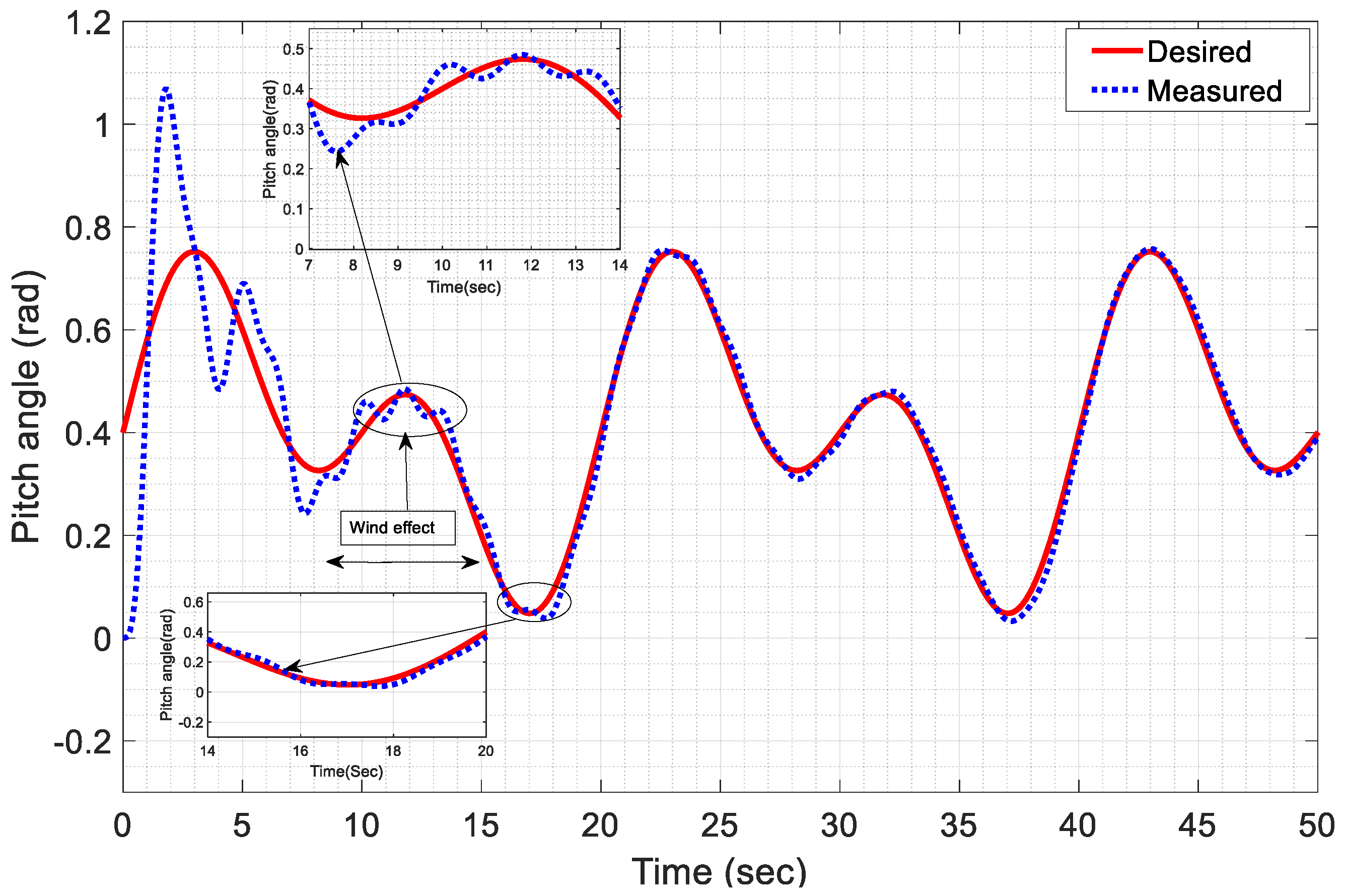
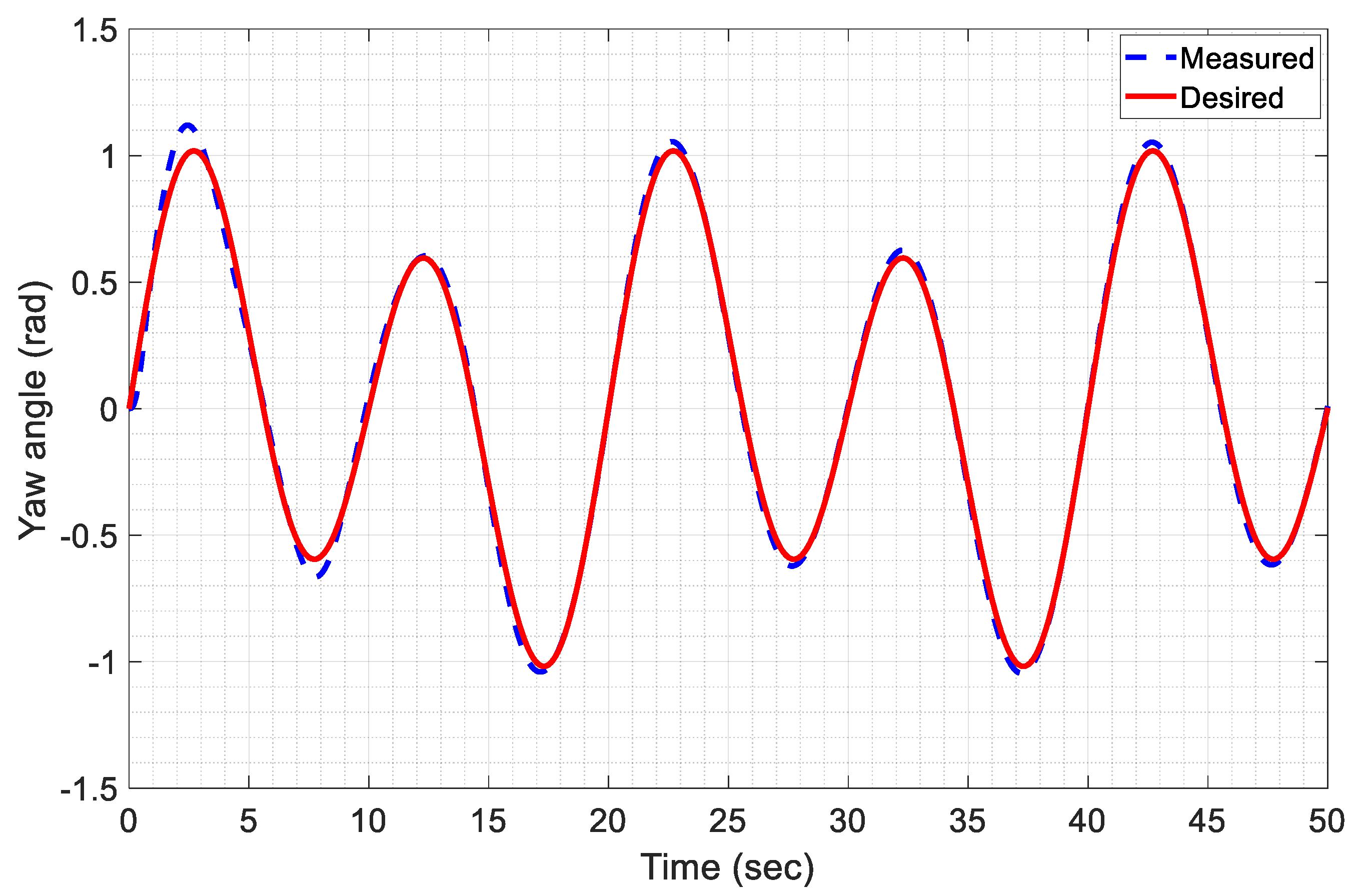
4.4.1. Real-Time Implementation with Input Sinusoidal Wave Trajectory Tracking in the Presence of Wind Effect for ISMC Law

Experimental validation of the IMSC law was accomplished using real-time TRMS with a reference input sinusoidal trajectory. Special blocks were used to read the attached encoder channel information using digital input and output lines. The block mainly contained three parameters: sample time, channel offset, and two channel offsets. The parameters of the PCI1711 card were set as follows: a sample time of 0.001 s and offset were initially considered zero for both channels. Channel one represents the output of the first encoder $\phi$ whereas channel two presents the second encoder $\psi$. The reference inputs selected for the pitch and yaw angles are given as

$$\begin{gathered} y_{1d}=0.7\sin \left(0.1t\right)+0.5\sin \left(4t\right)+0.2\sin \left(3t\right) \\ {y}_{2d}=\sin \left(t\right)+0.3\sin \left(0.4t\right)+0.55\sin \left(0.4t\right) \end{gathered}$$

Figure 24 and Figure 25 present the tracking response of the pitch and yaw angles, along with the control input effort for the ISMC. Figure 23 shows the obtained experimental results of the pitch angle tracking response when wind gusts are introduced to validate the robust performance of the controller. Three signal generators were used to adjust the frequencies of the reference angle, and three frequencies were set for the sinusoidal wave, i.e., signal generator 1 (0.0159 Hz), signal generator 2 (0.636 Hz) and signal generator 3 (0.4775 Hz). It was observed that the pitch angle efficiently tracked the reference input and stabilized the desired angle trajectory at $5 \mathrm{s}$. Initially, it could be observed that the pitch angle rapidly tracked the reference trajectory with a small overshoot and steady-state error. A gust disturbance effect was added to the pitch angle at time $t=8 \mathrm{s}$ to verify the robustness of the proposed controller. Furthermore, the pitch angle precisely tracked the reference trajectory after the application of external disturbances and explicitly maintained the output within $5.5 \mathrm{s}$. Consequently, the implemented technique guaranteed external disturbance rejection properties with good robustness and finite-time convergence.

Figure 25 shows the tracking performance of the yaw angle against the reference sinusoidal wave. It can be noted that the yaw angle was stable after $3.5 \mathrm{s}$ and the controller kept the measured angle close to the reference input signal. The frequencies of the input signal were adjusted from channels 1, 2 and 3. The obtained result illustrates that the yaw angle showed fast convergence towards the reference trajectory as compared to the pitch angle with a small overshoot of less than 1% and almost zero steady-state error. Moreover, the results obtained for both outputs demonstrated the effectiveness of the proposed control scheme.

Figure 26 shows the input control effort for the pitch and yaw angles. The voltage from DC motor and control signal are set at $[-2.5-2.5]$ volts, respectively, for control effort $u_{\phi }$ and $u_{\psi }$. Both control inputs reject external disturbances and demonstrate satisfactory performance in all respects. The initial peak occurred because of the discontinuous nature of sinusoidal waves. It can be observed that both control inputs remained within a predefined voltage-specified interval.

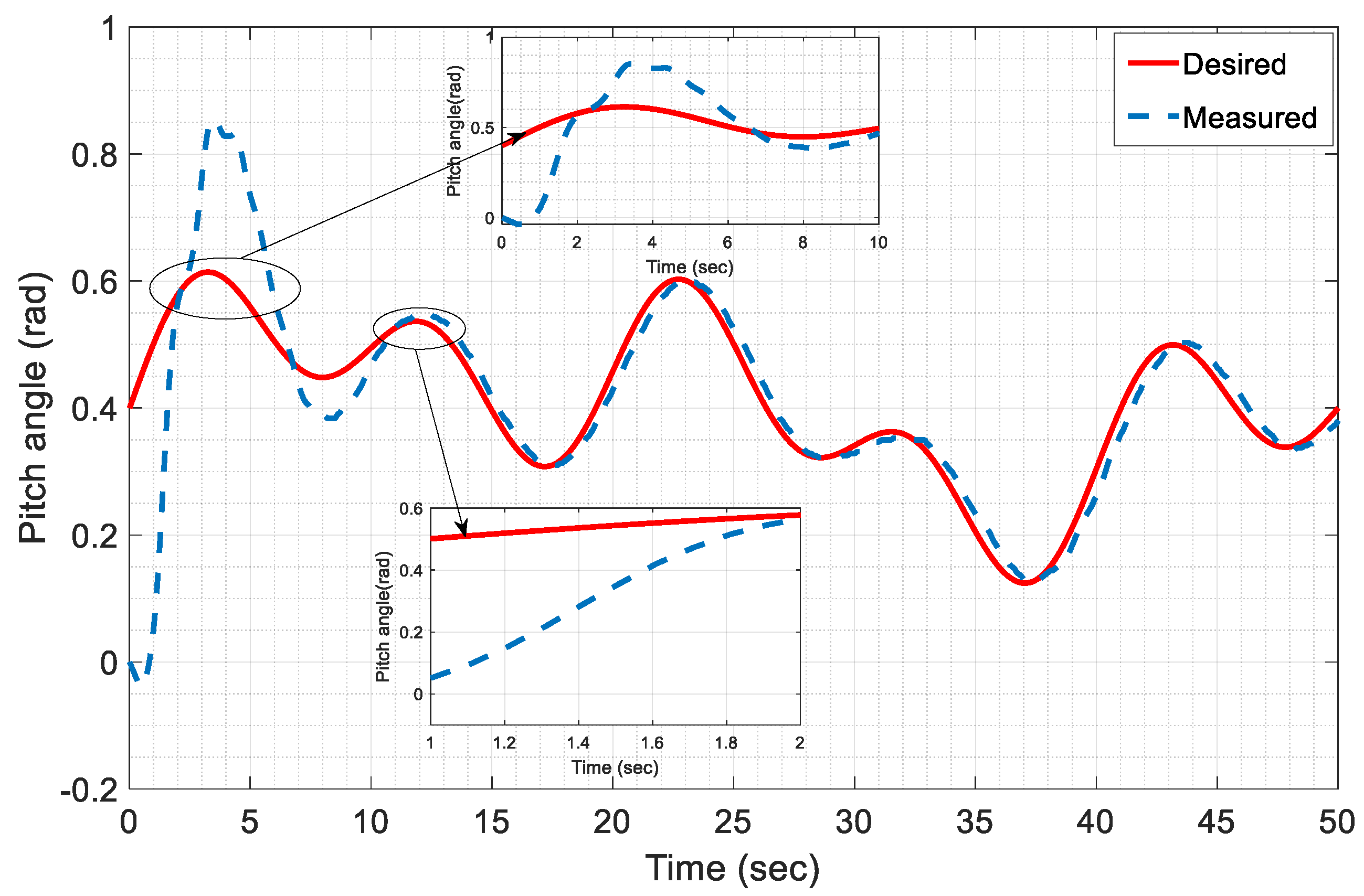
4.4.2. Input Sinusoidal Wave Trajectories Tracking for TSMC Law

To test the reliability and accuracy of TSMC reference input, sine wave signals were given to the controller with amplitudes of 0.7 rad, 0.5 rad and 0.2 rad, respectively, for the output of TRMS. Because of the involvement of the terminal sliding mode component, the TSMC has a complex control structure; therefore, after careful tuning of the real-time system parameters, the results were achieved. Figure 27 and Figure 28 illustrate the output response of the main and tail rotors along with the control efforts to investigate the performance of the TSMC law on a real-time TRMS. As shown in Figure 27 and Figure 28, both the pitch and yaw angles follow the reference input control signal and closely maintain both angles to the desired trajectories. The obtained results showed satisfactory transient performance, and very small overshoots and rise times were observed. The steady-state error between the actual and desired responses was minimal. The experimentally tested sharp responses of both outputs validate the accuracy and convergence of the controller. Initially, a small overshoot arose owing to the highly nonlinear dynamic nature of the system and the parametric perturbation. Frequencies of 0.1592 Hz, 0.0637 Hz and 0.0637 Hz were correspondingly considered for both the output angles by using the signal generators. It can be observed that after the transient deviation in real time tested the TSMC law results, the pitch angle was stable at time $t=8 \mathrm{s}$, while the yaw angle showed a relatively fast convergence at $t=7 \mathrm{s}$. The overshoot for the main angle was 4%, whereas that for the tail angle was 3%. This also exhibits a very precise steady-state error.

Figure 29 shows the control input performance of the main and tail rotors of TRMS. From the figure, we can observe that the input control voltage signal is restricted within the defined interval of $[-2.5-2.5]$ volts, which ensures that the minimum energy is consumed.

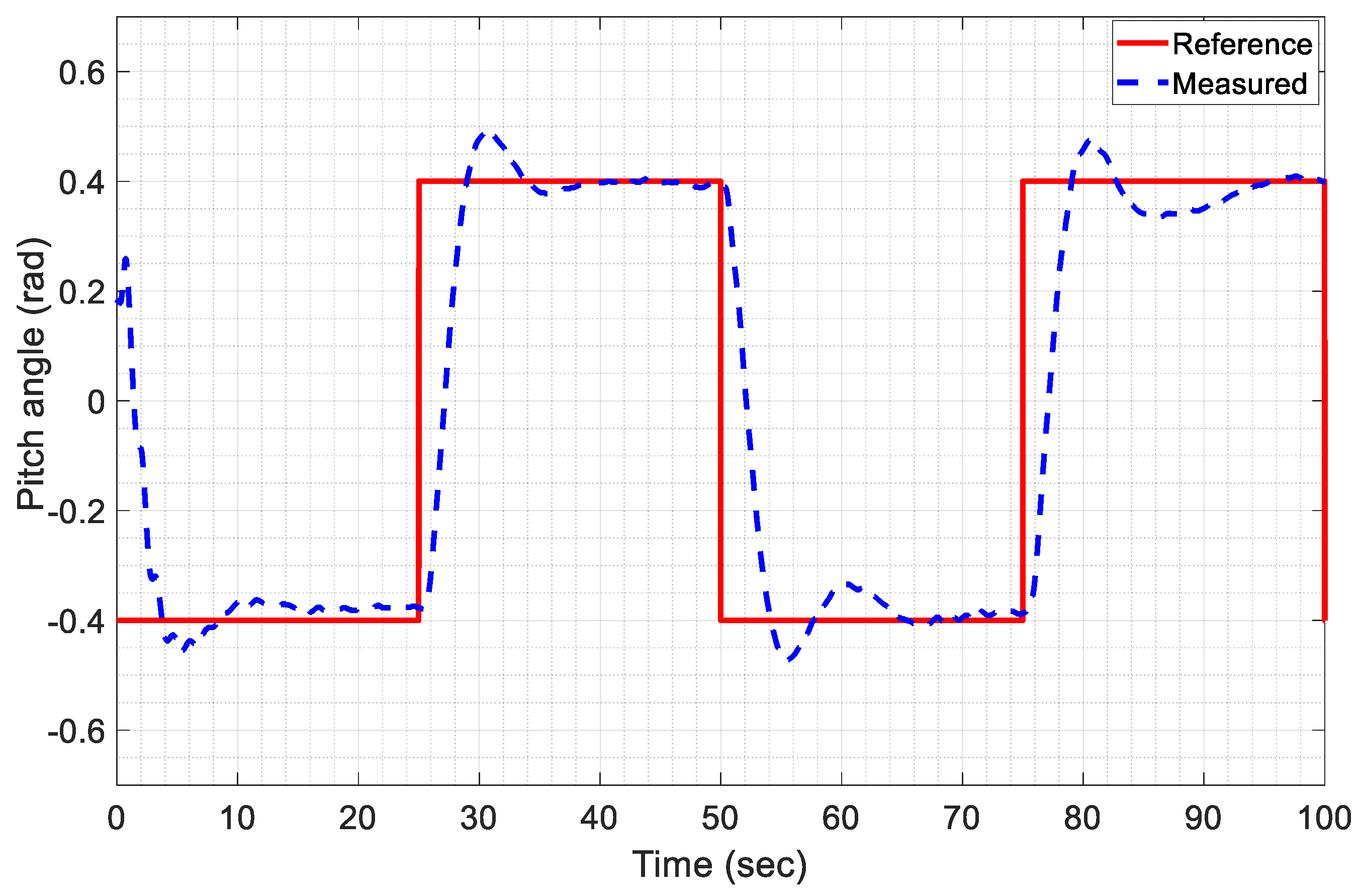
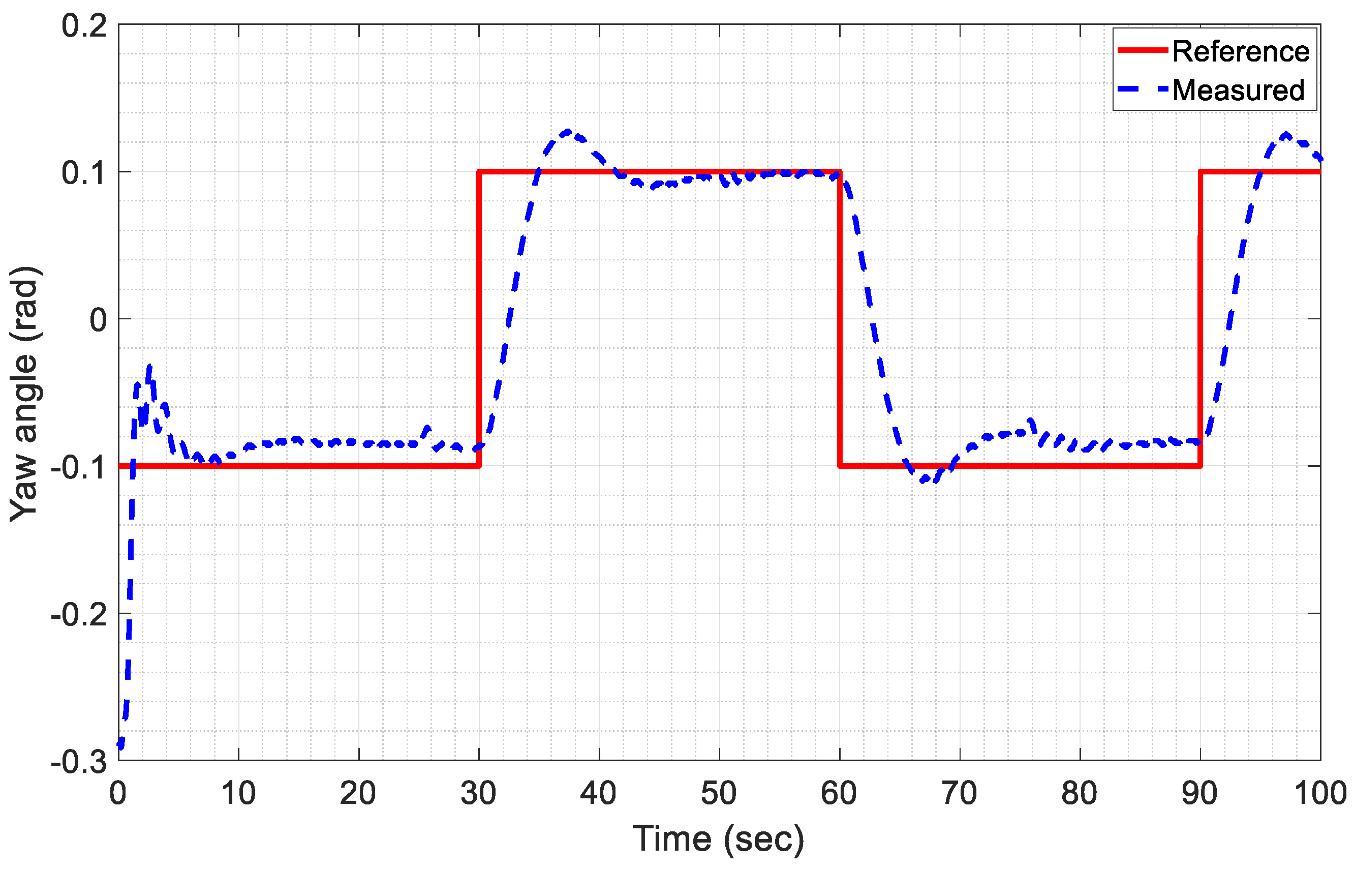
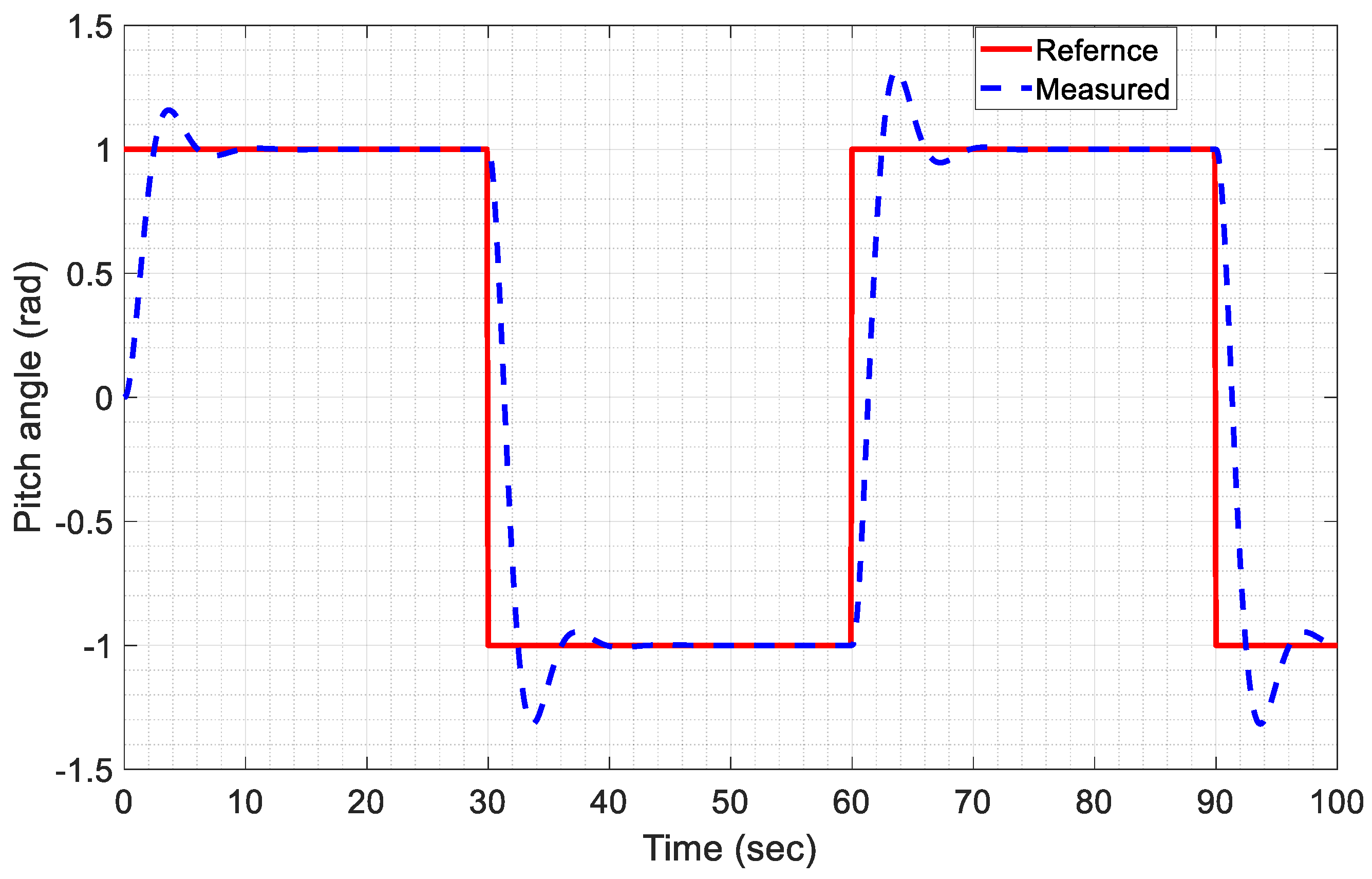
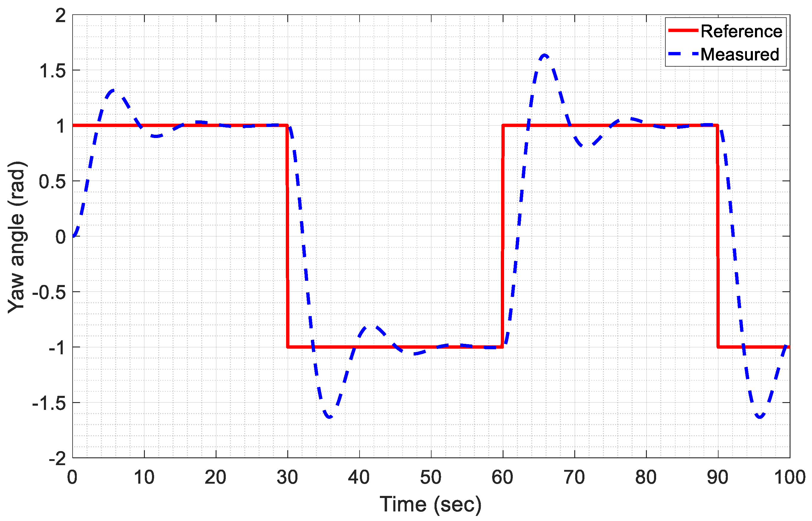
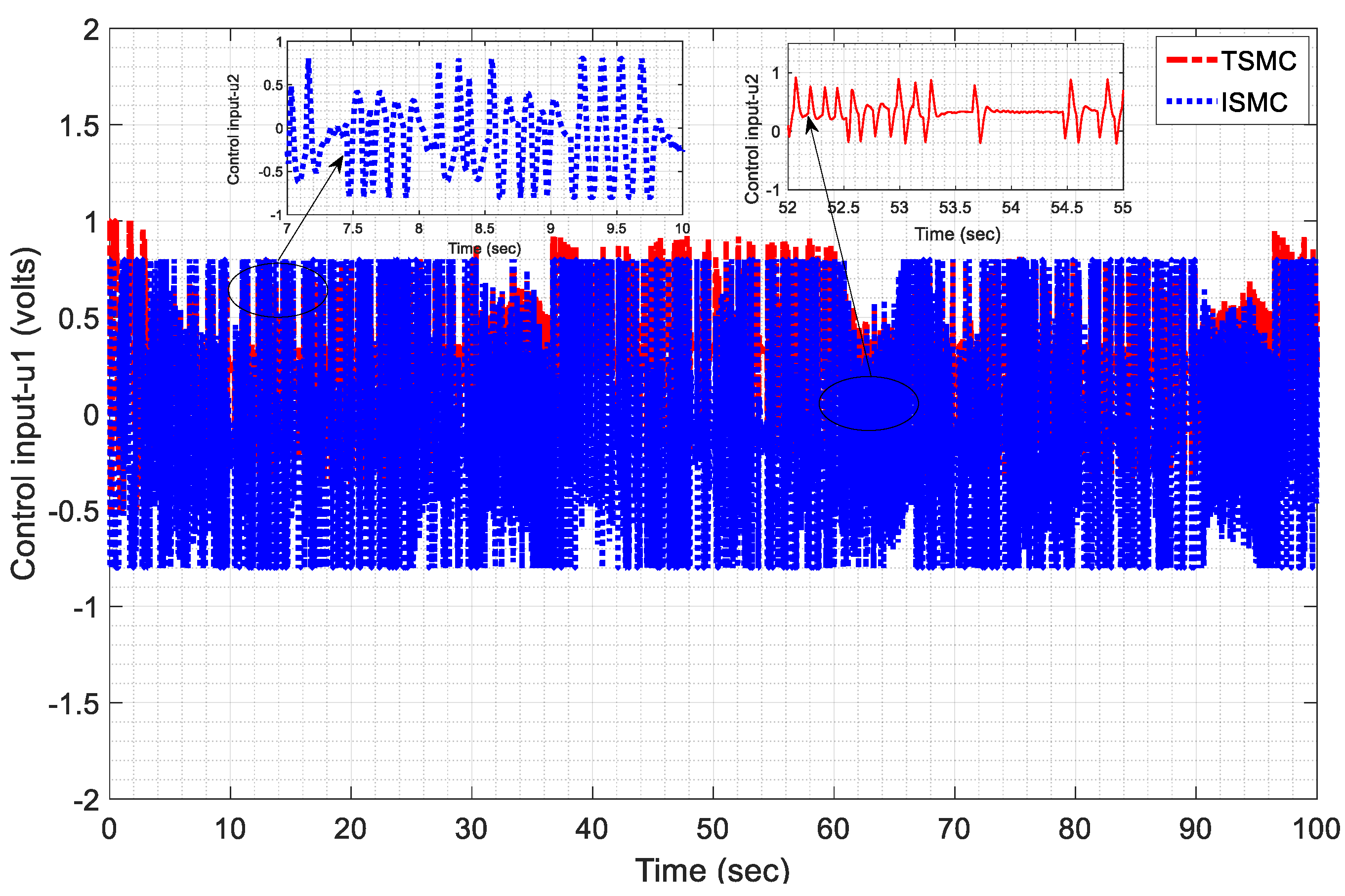
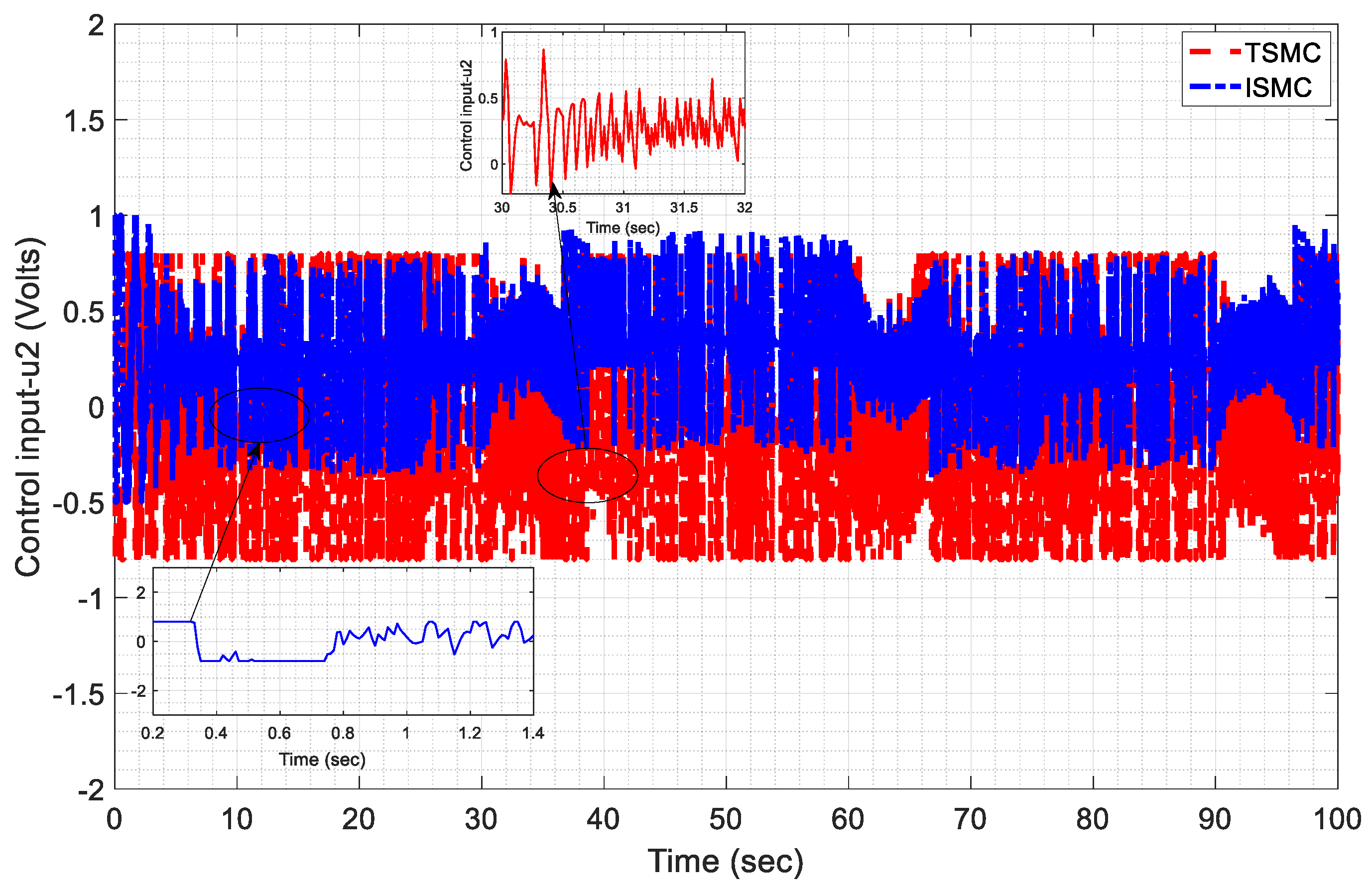
4.4.3. Real-Time Implementation of TSMC and ISMC Laws against the Square Wave

In this section, the results of real-time implementation and system interconnection for the TSMC and ISMC laws through a system-integrated circuit are presented. Furthermore, a succinct overview is provided based on the achieved output results to validate the performance of the controller. The real-time implementation of robustly designed control techniques demonstrates reliable performance in the presence of disturbances, noise signals, coupling effects, and parametric variations. Figure 22 and Figure 23 show the experimental setup and real-time implementation, respectively. Each diagram offers a comprehensive depiction of the process involved in the real-time implementation and provides insight into the laboratory hardware prototype.

The TSMC and ISMC laws were tested using various tuning parameters. The experimental output responses for the pitch and yaw angles against the square-wave tracking movement for the TSMC law are shown in Figure 30 and Figure 31, respectively. Both sets of results illustrate the capability of the controller to mitigate system variations while accurately tracking the reference input signal. The square wave reference input indicates that the pitch angle underwent smoother and quicker convergence in comparison to the yaw angle. This variation can be ascribed to the initial necessity of stabilizing the main rotor to counteract disturbances originating from the tail rotor, which include gyroscopic torque and coupling effects. Consequently, the convergence time for the pitch angle should be greater than that for the yaw angle. The responses of the main and tail rotors for the ISMC law are illustrated in Figure 32 and Figure 33, respectively, against the input square-wave trajectory. It should be noted that the convergence time of the pitch angle is faster than that of the yaw angle. Additionally, the pitch angle exhibits improved steady-state error, overshoot, and rise time compared with the yaw angle.

The control input signals for the main and tail rotors are shown in Figure 34 and Figure 35, respectively. The experimental control action responses for both angles can be characterized by minimal voltage fluctuations, highlighting the efficacy of the proposed controllers. The attenuation observed in the response can be attributed to the introduced noise signal and controller’s adept handling of a broad spectrum of disturbances. Moreover, the results demonstrate the controller’s gradual mitigation of the introduced disturbance over time, thereby enhancing system stability. In addition, both the control inputs remain within the predefined DC motor and control signal, which are set at $[-2.5-2.5]$ volts, thus guaranteeing the minimum consumption of energy.

To further evaluate the performance of the proposed controllers, integral performance indices and quantitative analyses were performed for all the proposed control algorithms, the results of which are presented below in

Table 6. Quantitative analysis of designed controller for TRMS.

Control Algorithms	Euler’s Angles	ISE (rad2/s)	IAE (rad/s)	ITSE (rad2/s2)	ITAE (rad/s)	$‖\mathit{u}‖$	${\mathit{u}}_{\mathit{a}\mathit{v}\mathit{g}}$	${\mathit{e}}_{\mathit{r}\mathit{m}\mathit{s}}$	${\mathit{e}}_{\mathit{M}\mathit{A}\mathit{E}}$
SMC	Pitch	180	$1.5 \times {10}^2$	0.66	50.55	10 × ${10}^4$	160	0.0095	0.020
	Yaw	350	$0.9 \times {10}^2$	0.83	25.25	8.4 × ${10}^4$	80	0.0055	0.051
ISMC	Pitch	120	$1.1 \times {10}^3$	0.19	25.1	9 × ${10}^2$	125	0.0011	0.0015
	Yaw	225	$0.8 \times {10}^3$	0.80	13.55	8.1 × ${10}^2$	29	0.0012	0.0049
TSMC	Pitch	123	$1.40 \times {10}^3$	0.50	26.5	9 × ${10}^2$	135	0.0045	0.0060
	Yaw	285	$0.88 \times {10}^3$	0.75	19.65	8.2 × ${10}^2$	40	0.0017	0.0058

and

Table 7. Quantitative analysis of ISMC and TSMC for experimental results.

Control Algorithms	Euler’s Angles	ISE (rad2/s)	IAE (rad/s)	ITSE (rad2/s2)	ITAE (rad/s)	$‖\mathit{u}‖$	${\mathit{u}}_{\mathit{a}\mathit{v}\mathit{g}}$	${\mathit{e}}_{\mathit{r}\mathit{m}\mathit{s}}$	${\mathit{e}}_{\mathit{M}\mathit{A}\mathit{E}}$
ISMC	Pitch	150.5	$1.11 \times {10}^2$	1.13	10.5	15	130	0.0019	0.75
	Yaw	95.5	$3.11 \times {10}^3$	3.12	20.21	9.5	155.5	0.011	0.97
TSMC	Pitch	80.6	$2.42 \times {10}^2$	0.95	25.12	27	180.5	0.0092	1.31
	Yaw	110.4	$5.11 \times {10}^3$	4.13	35.11	20	220.5	0.099	1.85

.

With careful consideration, the quantitative analysis and performance of different indices for simulations and real-time-implemented controllers for TRMS were performed, as presented in Table 6 and Table 7. Table 6 briefly explains the information on all the performance indices. It can be observed that the proposed control techniques provide a good response with a small IAE and ITSE for all control techniques. The ISMC provides a much better response for ISE, IAE, ITSE, and ITAE than the SMC, whereas the TSMC provides a more precise performance with a lower steady state than the SMC. Quantitative analysis demonstrated the performance of the control effort and smoothness with root mean square and absolute errors. The ISMC consumed less energy than the SMC and TSMC for the control action. Smoothness was also much better in the case of the ISMC compared to the other two controllers.

Table 7 presents the quantitative performance analysis and integral indices for the real-time tested control techniques of TRMS. It can be seen that both control techniques produce smooth tracking performance with higher IAE owing to the parameter convergence problem, whereas after the steady-state response, better performance is observed for ISE, ITSE, and ITAE. Energy consumption is proportional to the norm of the control effort $‖u‖$. Therefore, the calculated results predict that both control techniques consume minimal energy in real-time implementation against pitch and yaw angles. Similarly, the root-mean-square and maximum absolute error results are obtained accurately.

5. Conclusions

In this study, the research began by presenting the design of advanced nonlinear robust control algorithms that combine input–output feedback linearization, URED, and a state feedback observer, which were then validated through real-time TRMS experiments. The feedback linearization method effectively separates the highly interconnected system into horizontal and vertical subsystems. Brief SMC, ISMC, and TSMC control designs were produced to compare their performance, while the state feedback observer efficiently provided information on estimated states, and the URED measured unknown system states through estimation. The proposed control algorithms for TRMS demonstrate significant advancements and practical applications. By addressing the challenges of nonlinearity, coupling, and external disturbances, these control strategies enhance the performance and reliability of complex dynamical systems, making them highly relevant in various high-precision and safety-critical applications. All of the designed controllers exhibit robustness against uncertainties, encompassing nonlinearities and externally matched and unmatched disturbances. Additionally, ISMC and TSMC control techniques were implemented in real-time trials on TRMS, and concise discussions on their execution are provided. The proposed controllers demonstrate exceptional convergence and tracking performance in both simulations and real-time experimental testing, effectively steering the system output trajectories to the desired positions. Stability of state convergence was ensured using Lyapunov stability analysis. To comprehensively evaluate the results, transient responses and integral performance indices were analyzed through mathematical calculations. This is crucial for systems requiring high precision and fast dynamic response. Simulation assessments confirmed the robustness of the controllers against disturbances and nonlinearities. Notably, the chattering phenomena inherent in the SMC law were effectively mitigated by ISMC and TSMC. Both MATLAB/Simulink simulations and experimental trials validate the methodologies. Particularly, experimental studies showcase the impressive tracking response of the TRMS against wind gusts when employing ISMC law.

References

1. Guo, Z.; Yan, S.; Xu, X.; Chen, Z.; Ren, Z. Twin-model based on model order reduction for rotating motors. IEEE Trans. Magn. 2022, 58, 1–4. [Google Scholar] [CrossRef]
2. Haruna, A.; Mohamed, Z.; Abdullahi, A.M.; Basri, M.A.M. A Review of Control Algorithms for Twin Rotor Systems. Appl. Model. Simul. 2023, 7, 93–99. [Google Scholar]
3. Sivadasan, J.; Shiney, J.R.J. Modified nondominated sorting genetic algorithm-based multiobjective optimization of a cross-coupled nonlinear PID controller for a Twin Rotor System. J. Eng. Appl. Sci. 2023, 70, 133. [Google Scholar] [CrossRef]
4. Palepogu, K.R.; Mahapatra, S. Design of sliding mode control with state varying gains for a Benchmark Twin Rotor MIMO System in Horizontal Motion. Eur. J. Control 2024, 75, 100909. [Google Scholar] [CrossRef]
5. Srinivasarao, G.; Samantaray, A.K.; Ghoshal, S.K. Cascaded adaptive integral backstepping sliding mode and super-twisting controller for twin rotor system using bond graph model. ISA Trans. 2022, 130, 516–532. [Google Scholar] [CrossRef]
6. Abbas, N.; Pan, X.; Raheem, A.; Shakoor, R.; Arfeen, Z.A.; Rashid, M.; Umer, F.; Safdar, N.; Liu, X. Real-time robust generalized dynamic inversion based optimization control for coupled twin rotor MIMO system. Sci. Rep. 2022, 12, 17852. [Google Scholar] [CrossRef]
7. Charfeddine, S.; Alharbi, H.; Jerbi, H.; Kchaou, M.; Abbassi, R.; Leiva, V. A stochastic optimization algorithm to enhance controllers of photovoltaic systems. Mathematics 2022, 10, 2128. [Google Scholar] [CrossRef]
8. Mohammadzahri, M.; Khaleghifar, A.; Ghodsi, M.; Soltani, P.; AlSulti, S. A discrete approach to feedback linearization, yaw control of an unmanned helicopter. Unmanned Syst. 2023, 11, 57–66. [Google Scholar] [CrossRef]
9. Abbas, N.; Liu, X.; Iqbal, J. Robust GDI-based adaptive recursive sliding mode control (RGDI-ARSMC) for a highly nonlinear MIMO system with varying dynamics of UAV. J. Mech. Sci. Technol. 2024, 38, 2015–2028. [Google Scholar] [CrossRef]
10. Rashad, R.; El-Badawy, A.; Aboudonia, A. Sliding mode disturbance observer-based control of a twin rotor MIMO system. ISA Trans. 2017, 69, 166–174. [Google Scholar] [CrossRef]
11. Abbas, N.; Liu, X.; Iqbal, J. A flexible mixed-optimization with H∞ control for coupled twin rotor MIMO system based on the method of inequality (MOI)-An experimental study. PLoS ONE 2024, 19, e0300305. [Google Scholar] [CrossRef] [PubMed]
12. Isidori, A.; Astolfi, A. Disturbance attenuation and H/sub infinity/-control via measurement feedback in nonlinear systems. IEEE Trans. Autom. Control 1992, 37, 1283–1293. [Google Scholar] [CrossRef]
13. Pakro, F.; Nikkhah, A.A. A fuzzy adaptive controller design for integrated guidance and control of a nonlinear model helicopter. Int. J. Dyn. Control 2023, 11, 701–716. [Google Scholar] [CrossRef]
14. Singh, V.K.; Kamal, S.; Ghosh, S. Prescribed-time constrained feedback control for an uncertain twin rotor helicopter. Aerosp. Sci. Technol. 2023, 140, 108483. [Google Scholar] [CrossRef]
15. Dutta, L.; Kumar Das, D. Nonlinear disturbance observer-based adaptive feedback linearized model predictive controller design for a class of nonlinear systems. Asian J. Control 2022, 24, 2505–2518. [Google Scholar] [CrossRef]
16. Zheng, E.; Xiong, J. Quad-rotor unmanned helicopter control via novel robust terminal sliding mode controller and under-actuated system sliding mode controller. Optik 2014, 125, 2817–2825. [Google Scholar] [CrossRef]
17. Jiang, T.; Lin, D.; Song, T. Novel integral sliding mode control for small-scale unmanned helicopters. J. Frankl. Inst. 2019, 356, 2668–2689. [Google Scholar] [CrossRef]
18. Nonaka, K.; Sugizaki, H. Integral sliding mode altitude control for a small model helicopter with ground effect compensation. In Proceedings of the 2011 American Control Conference, San Francisco, CA, USA, 29 June–1 July 2011; pp. 202–207. [Google Scholar]
19. Butt, S.S.; Aschemann, H. Multi-variable integral sliding mode control of a two degrees of freedom helicopter. IFAC-PapersOnLine 2015, 48, 802–807. [Google Scholar] [CrossRef]
20. Fang, X.; Liu, F. High-order mismatched disturbance rejection control for small-scale unmanned helicopter via continuous nonsingular terminal sliding-mode approach. Int. J. Robust Nonlinear Control 2019, 29, 935–948. [Google Scholar] [CrossRef]
21. Fessi, R.; Bouallègue, S.; Haggège, J.; Vaidyanathan, S. Terminal sliding mode controller design for a quadrotor unmanned aerial vehicle. In Applications of Sliding Mode Control in Science and Engineering; Springer: Cham, Switzerland, 2017; pp. 81–98. [Google Scholar]
22. Krener, A.J.; Isidori, A. Linearization by output injection and nonlinear observers. Syst. Control Lett. 1983, 3, 47–52. [Google Scholar] [CrossRef]
23. Viana, K.; Larrea, M.; Irigoyen, E.; Diez, M.; Zubizarreta, A. MIMO neural models for a twin-rotor platform: Comparison between mathematical simulations and real experiments. In Proceedings of the 15th International Conference on Soft Computing Models in Industrial and Environmental Applications (SOCO 2020), Burgos, Spain, 16–18 September 2020; pp. 407–417. [Google Scholar]
24. Martinez-Armero, Y.; Renteria-Mena, J.B.; Giraldo, E. Robust Embedded Control applied to a Twin Rotor MIMO System. Eng. Lett. 2023, 31, 230–238. [Google Scholar]
25. Irfan, S.; Mehmood, A.; Razzaq, M.T.; Iqbal, J. Advanced sliding mode control techniques for inverted pendulum: Modelling and simulation. Eng. Sci. Technol. Int. J. 2018, 21, 753–759. [Google Scholar] [CrossRef]
26. Jia, Z.; Yu, J.; Mei, Y.; Chen, Y.; Shen, Y.; Ai, X. Integral backstepping sliding mode control for quadrotor helicopter under external uncertain disturbances. Aerosp. Sci. Technol. 2017, 68, 299–307. [Google Scholar] [CrossRef]
27. Hou, Z.; Yu, X.; Lu, P. Terminal sliding mode control for quadrotors with chattering reduction and disturbances estimator: Theory and application. J. Intell. Robot. Syst. 2022, 105, 71. [Google Scholar] [CrossRef]
28. Palepogu, K.R.; Mahapatra, S. Synchronous Pitch and Yaw Orientation Control of a Twin Rotor MIMO System Using State Varying Gain Sliding Mode Control. Arab. J. Sci. Eng. 2024, 1–14. [Google Scholar] [CrossRef]
29. Rezoug, A.; Messah, A.; Messaoud, W.A.; Baizid, K.; Iqbal, J. Adaptive-optimal MIMO nonsingular terminal sliding mode control of twin-rotor helicopter system: Meta-heuristics and super-twisting based control approach. J. Braz. Soc. Mech. Sci. Eng. 2024, 46, 162. [Google Scholar] [CrossRef]
Figure 1. Physical model of twin rotor system.
Drones 08 00527 g001
Figure 2. Block diagram of dynamics cross-coupling in TRMS.
Drones 08 00527 g002
Figure 3. Closed-loop block diagram of proposed control strategies.
Drones 08 00527 g003
Figure 4. Closed-loop block diagram of nonlinear state feedback observer for ISMC law.
Drones 08 00527 g004
Figure 5. Pitch angle response with disturbance.
Drones 08 00527 g005
Figure 6. Yaw angle response with disturbance.
Drones 08 00527 g006
Figure 7. Control input u 1 response with disturbance.
Drones 08 00527 g007
Figure 8. Control input u 2 response with disturbance.
Drones 08 00527 g008
Figure 9. Pitch angle tracking response with sine wave.
Drones 08 00527 g009
Figure 10. Yaw angle tracking response with sine wave.
Drones 08 00527 g010
Figure 11. Control input u 1 for sine wave.
Drones 08 00527 g011
Figure 12. Control input u 2 for sine wave.
Drones 08 00527 g012
Figure 13. Tracking error for pitch angle.
Drones 08 00527 g013
Figure 14. Tracking error for yaw angle.
Drones 08 00527 g014
Figure 15. Pitch angle response for step input.
Drones 08 00527 g015
Figure 16. Yaw angle response for step input.
Drones 08 00527 g016
Figure 17. Pitch angle u 1 response for step input.
Drones 08 00527 g017
Figure 18. Pitch angle u 2 response for step input.
Drones 08 00527 g018
Figure 19. ISMC-based observer responses for pitch and yaw angles.
Drones 08 00527 g019
Figure 20. Observer response for actuator fault.
Drones 08 00527 g020
Figure 21. URED velocity information for pitch ( Z ˙ 2 a ) and yaw ( Z ˙ 2 b ).
Drones 08 00527 g021
Figure 22. Experimental setup and test bench for TRMS.
Drones 08 00527 g022
Figure 23. Schematic diagram for experimental setup.
Drones 08 00527 g023
Figure 24. Experimental pitch angle tracking response for ISMC.
Drones 08 00527 g024
Figure 25. Experimental yaw angle tracking response for ISMC.
Drones 08 00527 g025
Figure 26. Experimental control input u 1 , u 2 response for ISMC.
Drones 08 00527 g026
Figure 27. Experimental pitch angle tracking response for TSMC.
Drones 08 00527 g027
Figure 28. Experimental yaw angle tracking response for TSMC.
Drones 08 00527 g028
Figure 29. Experimental control input u 1 , u 2 response for TSMC.
Drones 08 00527 g029
Figure 30. Experimental pitch angle square wave tracking response for TSMC.
Drones 08 00527 g030
Figure 31. Experimental yaw angle square wave tracking response for TSMC.
Drones 08 00527 g031
Figure 32. Experimental pitch angle square wave tracking response for ISMC law.
Drones 08 00527 g032
Figure 33. Experimental yaw angle square wave tracking response for ISMC law.
Drones 08 00527 g033
Figure 34. Experimental control input u 1 response for TSMC and ISMC.
Drones 08 00527 g034
Figure 35. Experimental control input u 2 response for TSMC and ISMC.
Drones 08 00527 g035